UMHEP 96–021
The Multichannel Quark Model

Abstract

We discuss the non–relativistic multichannel quark model and describe the techniques developed to solve the resulting equations. We then investigate some simple solutions to demonstrate how the model unifies meson–meson scattering with meson spectroscopy, thereby greatly extending the domain of applicability of the naïve quark model. In the limits of narrow resonance widths and no quark exchange, it reproduces the standard quark model spectroscopy and Breit–Wigner phase description. Outside those limits $s$–channel resonance masses are lowered by their two–meson couplings, the line–shapes of wide resonances are significantly altered, and the equivalent Breit–Wigner masses and widths show an energy dependence. Because meson–meson interactions are due to coherent $s$–channel resonance production and $t$–channel quark exchange (though other interactions can readily be added), the multichannel equations model experimental resonance production and decay in a way that the usual eigenvalue equations cannot.

I INTRODUCTION

The quark model attempts to represent the main features of QCD, the theory of quarks and gluons, and has been successfully used to calculate hadron spectroscopy and decays [3]. However, after decades of study, and numerous extensions, a multitude of discrepancies still remain between theory and experiment, particularly in the light meson sector.

In this paper we construct and solve a multichannel quark model, which we apply to meson–meson scattering. We consider only low energy scattering processes, which are resonably soft for all mesons except the $\pi$ at the high end of our energy range, so we use a non–relativistic formulation. We motivate the model phenomenologically by considering strong decay processes, and add terms representing these processes to the naïve quark model. Numerical solutions, which are described in the Appendicies, yield the $S$–matrix parameters for the free two–meson states and the masses, widths, and two–meson decay predictions for the $s$–channel meson resonances. The standard quark model spectroscopy and the Breit–Wigner phase shift [4] are reproduced, in the limits of narrow resonance width and vanishing quark exchange. Outside those limits resonance properties are found to depend significantly on two–meson couplings, which leads to mass shifts, energy dependent Breit–Wigner parameters, and two–meson bound states.

The paper is organized as follows: We first review spectroscopy in the naïve quark model. Next we develop the multichannel equation for the simple case of the elastic scattering of two stable mesons, $A$ and $B$, through an intermediate resonance $R$. Some qualitative behaviours of the solutions are explored, new effects are highlighted, and likely avenues of further investigations are noted. We then review the quark exchange process and incorporate it into the multichannel model. Finally we apply the model to inelastic multichannel scattering.

This model has been discussed previously in the square well approximation [5, 6] and, in a less complete form in [7]. See also [8].

The fortran source code that has been developed to find the numerical solutions to the multichannel equations, and rudimentary intructions for running it, are available over the World Wide Web [9].

II THE NAÏVE QUARK MODEL

One method of predicting the meson spectrum from the naïve quark model is to solve the eigenvalue problem

$$\vskip 12.0pt plus 4.0pt minus 4.0ptH_{\scriptscriptstyle\!R_{q\bar{q}}}({\bf r}_{q\bar{q}})\,\psi_{\scriptscriptstyle\!R_{q\bar{q}}}({\bf r}_{q\bar{q}})=m_{\scriptscriptstyle\!R}\,\psi_{\scriptscriptstyle\!R_{q\bar{q}}}({\bf r}_{q\bar{q}})\vskip 12.0pt plus 4.0pt minus 4.0pt$$ (1)

for each ${q\bar{q}}$ meson resonance $R$. Here the ${q\bar{q}}$ Hamiltonian $H_{\scriptscriptstyle\!R_{q\bar{q}}}({\bf r}_{q\bar{q}})$ defines all the properties of $R$. In the naïve quark model we use a phenomenological ${q\bar{q}}$ central potential $V_{\scriptscriptstyle\!R_{q\bar{q}}}({r_{{q\bar{q}}}})$, so that equation (1) becomes

$$\vskip 12.0pt plus 4.0pt minus 4.0ptH_{\scriptscriptstyle\!R_{q\bar{q}}}({\bf r}_{q\bar{q}})=\left[-{\hbar^{2}\over{2m}}{\bf\nabla\cdot\nabla}\right]\,+m_{q}\,+\,m_{\bar{q}}\,+V_{\scriptscriptstyle\!R_{q\bar{q}}}\,({r_{{q\bar{q}}}})\,,\vskip 12.0pt plus 4.0pt minus 4.0pt$$ (2)

where $V_{\scriptscriptstyle\!R_{q\bar{q}}}({r_{{q\bar{q}}}})$ takes the simple form

$$\vskip 12.0pt plus 4.0pt minus 4.0ptV_{\scriptscriptstyle\!R_{q\bar{q}}}\,({r_{{q\bar{q}}}})= - \!\!\Biggl{[}\,{3\over 4}\,b\,{r_{{q\bar{q}}}}\,-{\alpha_{c}\over{r_{{q\bar{q}}}}}\,-\alpha_{g}\,{\sigma_{g}^{3}\over\pi^{\scriptscriptstyle 3/2}}\,e^{-\sigma_{g}^{2}{r_{{q\bar{q}}}}^{2}}\,+{3\over 4}\,C\Biggr{]}\,{\,{\bf F}_{q}\cdot{\bf F}_{\bar{q}}}$$ (3)

$$- {8\pi\over 3}{\alpha_{h}\over m_{q}m_{\bar{q}}}\,{\sigma_{h}^{3}\over\pi^{\scriptscriptstyle 3/2}}\,e^{-\sigma_{h}^{2}{r_{{q\bar{q}}}}^{2}}\,{\bf S}_{q}\cdot{\bf S}_{\bar{q}}\,{\,{\bf F}_{q}\cdot{\bf F}_{\bar{q}}}\,.\vskip 12.0pt plus 4.0pt minus 4.0pt$$ (4)

The eight components of ${\bf F}_{q}$ (${\bf F}_{\bar{q}}$) are defined by $[{\bf F}_{q}]^{a}={1\over 2}{\bf\lambda^{a}}$ ($[{\bf F}_{\bar{q}}]^{a}=-{1\over 2}(\lambda^{a})^{*}$), for $a=1,8$, where the $\lambda^{a}$ are the eight 3x3 SU(3) color matricies. The ${\bf S}_{q}$ and ${\bf S}_{\bar{q}}$ are defined by $[{\bf S}_{q}]^{i}=[{\bf S}_{\bar{q}}]^{i}={1\over 2}\sigma^{i}$, for $i=1,3$, where the $\sigma$ are the three 2x2 SU(2) spin matricies. The expectation value of the ${\,{\bf F}_{q}\cdot{\bf F}_{\bar{q}}}$ factor reduces to a constant factor of $-4/3$ for mesons, while $\langle{\bf S}_{q}\cdot{\bf S}_{\bar{q}}\rangle=-3/4$ for spin zero ${q\bar{q}}$ systems and +1/4 for spin 1 systems [3].

The linear confinement term ($br_{q\bar{q}}$) is predicted by the flux–tube model and by lattice QCD. The $\alpha_{c}/{r_{{q\bar{q}}}}$ term is a short–range Coulomb piece that dominates the interaction when $r_{q\bar{q}}\ll$ 1 fm. It can also be represented by a short range gaussian potential, which approximates the mid– and long–range behaviour of the $1/{r_{{q\bar{q}}}}$ interaction, but is finite at ${r_{{q\bar{q}}}}=0$. $C$ is a constant background potential. The last term is the short–range color magnetic hyperfine interaction. It increases (decreases) the energy of systems whose color magnetic moments are aligned (anti–aligned). We ignore spin–orbit coupling terms, which normally lead to mass splitting of order 10 MeV between, for example, the ${}^{3}P_{0}$, ${}^{3}P_{1}$, and ${}^{3}P_{2}$ states. In Section III we will show, for the $\ell_{q\bar{q}}=1$, $s_{q\bar{q}}=1$, $K_{0}$, $K_{1}$, and $K_{2}$ states specifically, that different couplings and different external two–meson states shift the underlying ${q\bar{q}}$ resonance masses by 10s of MeV.

If we use separation of variables to write the ${q\bar{q}}$ wavefunction as

$$\vskip 12.0pt plus 4.0pt minus 4.0pt\psi_{\scriptscriptstyle\!R_{q\bar{q}}}({\bf r}_{q\bar{q}})={u_{\scriptscriptstyle\!R_{q\bar{q}}}({r_{{q\bar{q}}}})}\,{1\over r_{q\bar{q}}}\,Y_{\scriptscriptstyle\!R_{q\bar{q}}}(\theta,\phi)\vskip 12.0pt plus 4.0pt minus 4.0pt$$ (5)

then $u_{\scriptscriptstyle\!R_{q\bar{q}}}({r_{{q\bar{q}}}})$ obeys the radial equation [10]

$$\vskip 12.0pt plus 4.0pt minus 4.0ptH_{\scriptscriptstyle\!R_{q\bar{q}}}({r_{{q\bar{q}}}})\,u_{\scriptscriptstyle\!R_{q\bar{q}}}({r_{{q\bar{q}}}})=m_{\scriptscriptstyle\!R}\,u_{\scriptscriptstyle\!R_{q\bar{q}}}({r_{{q\bar{q}}}})\vskip 12.0pt plus 4.0pt minus 4.0pt$$ (6)

where $H_{\scriptscriptstyle\!R_{q\bar{q}}}({r_{{q\bar{q}}}})$ is the radial part of the ${q\bar{q}}$ Hamiltonian given by

$$\vskip 12.0pt plus 4.0pt minus 4.0ptH_{\scriptscriptstyle\!R_{q\bar{q}}}(r_{q\bar{q}})=-{\hbar^{2}\over 2\,\mu_{{q\bar{q}}}}{{\rm d}^{2}\over{\rm d}{r_{{q\bar{q}}}}\,^{2}}+{\hbar^{2}\over 2\,\mu_{{q\bar{q}}}}\,{\ell_{q\bar{q}}(\ell_{q\bar{q}}+1)\over{r_{{q\bar{q}}}}^{2}}\,+m_{q}\,+\,m_{\bar{q}}\,+V_{\scriptscriptstyle\!R_{q\bar{q}}}\,({r_{{q\bar{q}}}}).\vskip 12.0pt plus 4.0pt minus 4.0pt$$ (7)

In (7) $\mu_{q\bar{q}}$ is the reduced ${q\bar{q}}$ mass, given by $\mu_{q\bar{q}}=2m_{\scriptscriptstyle q}m_{\scriptscriptstyle\bar{q}}/(m_{\scriptscriptstyle q}+m_{\scriptscriptstyle\bar{q}})$. The second term is the centrifugal barrier term, which comes from the three dimensional kinetic energy operator. Since we limit ourselves to this one–dimensional equation, we choose to view the barrier term as part of the potential, rather than part of the kinetic energy.

Solutions of equation (6) yield meson masses $m_{\scriptscriptstyle\!R}$ and meson wavefunctions $u_{\scriptscriptstyle\!R_{q\bar{q}}}({r_{{q\bar{q}}}})$ which, here, depend on quark flavor, ${q\bar{q}}$ separation ${r_{{q\bar{q}}}}$, spin $s_{q\bar{q}}$, and orbital angular momentum $\ell_{q\bar{q}}$. The light quark sector of this Hamiltonian has ten parameters, $m_{u}$, $m_{d}$, $m_{s}$, $b$, $\alpha_{c}$, $\alpha_{g}$, $\sigma_{g}$, $C$, $\alpha_{h}$, and $\sigma_{h}$, which are fixed so the model reproduces a small subset of the available data. Predictions for the masses of all other light mesons follow.

As we are using constituent, rather than current quark masses, we impose the constraint $m_{u}\!=\!m_{d}$, reducing the number of parameters to nine. We also choose $\alpha_{g}=0$, so the value of $\sigma_{g}$ becomes irrelevant, and we have seven free parameters.

In this paper we use $m_{u}=m_{d}=0.375$ GeV, $m_{s}=0.650$ GeV, $b=0.782$ GeV/fm, $\alpha_{c}=0.857$, $C=-0.581$ GeV, $\alpha_{h}=0.840$, and $\sigma_{h}=0.700$ GeV, which leads to the meson masses quoted below.

In Section III we will add two more parameters that couple ${q\bar{q}}$ resonances and two–meson states, and the scattering properties of two–meson systems can then be determined.

The wavefunctions $u_{\scriptscriptstyle\!R_{q\bar{q}}}({r_{{q\bar{q}}}})$ solving equation (6) are found numerically by finite difference methods using the Noumerov technique [11]. The details are provided in Appendix A. In the large $r$ region, these numerical solutions are, generally, linear combinations of an exponentially decaying and an exponentially growing term. The relative amplitude of each term depends on the trial energy $E_{\scriptscriptstyle\!R}$. The physical solutions are defined by the additional constraint that $u_{\scriptscriptstyle\!R}({r_{{q\bar{q}}}})\to 0$ as ${{r_{{q\bar{q}}}}\to\infty}$, which requires that the amplitude of the exponentially growing factor vanish, and defines the eigenenergies ${m_{\scriptscriptstyle\!R}}$. Details are given in Appendix B.

In FIG. 1. we plot the $\ell_{q\bar{q}}=1$, $s_{q\bar{q}}=1$, $K_{J=0,1,2}$ radial wavefunctions at trial energies of $E_{1}=1.4299235012$ GeV and $E_{2}=1.4299235014$ GeV. (We have no spin–orbit term in the Hamiltonian, so the $K_{J}$’s are degenerate at this point.) The lower energy solution goes to $+\infty$ as ${r_{{q\bar{q}}}}\to\infty$ while the other solution, which is only 0.2 eV greater in energy, goes to $-\infty$ as ${r_{{q\bar{q}}}}\to\infty$! The eigenenergy lies somewhere in between these two values, so we can clearly use this proceedure to determine the eigenenergies of (6) to an irrelevantly high accuracy.

As a verification of this technique we tested the iterating program on the toy problem of two quarks confined by an harmonic oscillator potential. We found that the trial energies differ from the exact analytic eigenenergies by less than one part in $10^{11}$, and the numerical wavefunctions differ from the exact gaussian solutions by less than one part in $10^{8}$ out to distances of 8 fm! The harmonic oscillator is a particularly simple potential however, and we must always check the solutions to make sure they are independent of the various iteration parameters introduced to numerically solve equation (6).

In FIG. 2. we show the wavefunction of the first radial excitation of the $K_{J}$ at energies of $E_{1}=2.047471763$ GeV and $E_{2}=2.047471768$ GeV. This energy resolution of 5 eV is coarser than above simply to make the wavefunctions diverge a distances of less than 6.0 fm. (As the trial energy approaches the eigenenergy the point of divergence of the trial wavefunction moves further from the origin.) The second radial excitation is at 2.5651608366 GeV, and the higher radial excitations are easily found this way.

With the Hamiltonian parameters above, this approach yields meson masses (in GeV) of $m_{\pi}=0.133$, $m_{K}=0.494$, $m_{\rho}=0.775$, $m_{K^{*}}=0.913$, $m_{\phi}=1.019$, $m_{b_{1}}=1.230$, $m_{K_{1}}=1.389$, $m_{h^{\prime}_{1}}=1.512$, $m_{a_{J}}=1.280$, $m_{K_{J}}=1.430$, and $m_{f^{\prime}_{J}}=1.550$, with J=1, 2, and 3, in good agreement with experiment.

III s–CHANNEL MESON RESONANCE PRODUCTION

When solving any ${q\bar{q}}$ eigenvalue problem one implicitly assumes that resulting mesons have a unique energy, and are therefore stable. However, most hadrons are hadronically unstable, with typical widths of 200 MeV. The Heisenberg uncertainty principal gives them a lifetime of

$$\vskip 12.0pt plus 4.0pt minus 4.0pt\tau\approx{\hbar\over\Delta E}\approx 10^{-15}{\rm fm}\approx 3\,{\rm x}\,10^{-24}{\rm sec}\,,\vskip 12.0pt plus 4.0pt minus 4.0pt$$ (8)

or as long (short) as it takes light to cross a meson. The zero width approximation intrinsic to the eigenvalue formulation is, therefore, unrealistic for all the hadronically decaying hadrons.

When we try to extract the spectroscopy of wide and interfering hadrons, glueballs, and hybrids from experimental data, as a means of gathering information about the underlying quark–quark interactions, and to test theories of QCD, we find the predictions of equation (6) inconsistent with data. There are results, such as the presence of two $\rho^{\prime}$ states, which have remained unexplained after years of intense research and many extensions of (6).

The multichannel model we propose scatters two–meson states into two–meson states through $s$–channel resonance production and $t$–channel quark exchange. The relative wavefunction of two–meson system, and the wavefunction of $s$–channel resonance, are found. From these the $S$–matrix and the resonance parameters are deduced.

Consider $s$–channel meson resonance formation. As an idealized gedanken scattering experiment one might think of two mesons, $A$ and $B$, coalescing via ${q\bar{q}}$ annihilation to form a single meson resonance $R$. (We will include the $t$–channel quark exchange effects below.) Some time later $R$ decays, via ${q\bar{q}}$ creation, into a final two–meson system $CD$, where $CD$ may or may not represent the same mesons as $AB$. This is depicted in FIG. 3.

For the moment we restrict our discussion to the elastic scattering process $AB\to R\to AB$. Consider the initial state $AB$ in FIG. 3. The Schrödinger equation, which determines the relative $AB$ wavefunction $u_{\scriptscriptstyle\!AB}(r_{\scriptscriptstyle\!AB})$, is

$$\vskip 12.0pt plus 4.0pt minus 4.0ptH_{\scriptscriptstyle\!AB}({r_{{\scriptscriptstyle\!AB}}})\,u_{\scriptscriptstyle\!AB}({r_{{\scriptscriptstyle\!AB}}})\,=E_{\scriptscriptstyle\!AB}\,u_{\scriptscriptstyle\!AB}({r_{{\scriptscriptstyle\!AB}}})\,,\vskip 12.0pt plus 4.0pt minus 4.0pt$$ (9)

where the radial part of the two–meson Hamiltonian $H_{\scriptscriptstyle\!AB}({r_{{\scriptscriptstyle\!AB}}})$ is given by

$$\vskip 12.0pt plus 4.0pt minus 4.0ptH_{\scriptscriptstyle\!AB}({r_{{\scriptscriptstyle\!AB}}})=-{\hbar^{2}\over 2\,\mu_{{\scriptscriptstyle\!AB}}}\left(\,{{\rm d}^{2}\over{\rm d}{r_{{\scriptscriptstyle\!AB}}}\,^{2}}\,-{\ell_{\scriptscriptstyle\!AB}(\ell_{\scriptscriptstyle\!AB}+1)\over{r_{{\scriptscriptstyle\!AB}}}^{2}}\right)\,+V_{\scriptscriptstyle\!AB\leftrightarrow AB}({r_{{\scriptscriptstyle\!AB}}})\,+m_{\scriptscriptstyle\!A}\,+m_{\scriptscriptstyle\!B}\,.\vskip 12.0pt plus 4.0pt minus 4.0pt$$ (10)

We have included the meson masses, $m_{\scriptscriptstyle\!A}$ and $m_{\scriptscriptstyle\!B}$, in the Hamiltonian so that the energy $E_{\scriptscriptstyle\!AB}$ represents the total energy of the $AB$ system in its center of momentum frame. The potential $V_{\scriptscriptstyle\!AB\leftrightarrow AB}$ will represent other possible non–resonant $AB$ interactions, such as quark exchange shown in FIG. 4., and will be discussed in Section VI. For the moment we take $V_{\scriptscriptstyle\!AB\leftrightarrow AB}=0$.

Equation (9) says that the $AB$ energy operator, $H_{\scriptscriptstyle\!AB}$, acting on the $AB$ probability amplitude, $u_{\scriptscriptstyle\!AB}({r_{{\scriptscriptstyle\!AB}}})$, equals the availiable energy $E_{\scriptscriptstyle\!AB}$ times $u_{\scriptscriptstyle\!AB}({r_{{\scriptscriptstyle\!AB}}})$. When one looks at the transition $AB$ to $R$ in FIG. 3., however, one sees that $R$ removes energy from $AB$. This suggests modifying equation (9) by removing a separation dependent energy factor, $V_{\scriptscriptstyle\!AB\to R}({r_{{\scriptscriptstyle\!AB}}})\,u_{q\bar{q}}({r_{{q\bar{q}}}})$, from the right hand side of (9), leading to

$$\vskip 12.0pt plus 4.0pt minus 4.0ptH_{\scriptscriptstyle\!AB}\,u_{\scriptscriptstyle\!AB}({r_{{\scriptscriptstyle\!AB}}})\ =E_{\scriptscriptstyle\!AB}\,u_{\scriptscriptstyle\!AB}({r_{{\scriptscriptstyle\!AB}}})\\ \,-V_{\scriptscriptstyle\!AB\to R}({r_{{\scriptscriptstyle\!AB}}})\,u_{q\bar{q}}({r_{{q\bar{q}}}}).\vskip 12.0pt plus 4.0pt minus 4.0pt$$ (11)

A standard model for ${q\bar{q}}$ annihilation couples the ${q\bar{q}}$ state to the vacuum, which requires that the annihilating ${q\bar{q}}$ pair be in an $\ell_{q\bar{q}}=1$, $s_{q\bar{q}}=1$, ${}^{3}P_{0}$ color singlet state [12, 13]. It is, however, possible that some annihilation verticies are dominated by the process ${q\bar{q}}\to g$ (where this $g$ is a gluon). This would require that the annihilating ${q\bar{q}}$ pair have the ${}^{3}S_{1}$ quantum numbers of the gluon, constraining them to an $\ell_{q\bar{q}}=0$, $s_{q\bar{q}}=1$, color octet state, and making $R$ a hybrid (${q\bar{q}}g$) meson. The model we are exploring here can be adapted to quantitatively study this fundamental question, though we do not do so here.

In this paper we choose, as an ansatz for the creation and annihilation verticies, the transition potential

$$\vskip 12.0pt plus 4.0pt minus 4.0ptV_{\scriptscriptstyle\!AB\to R}({r_{{\scriptscriptstyle\!AB}}})=g\,C^{f}_{\scriptscriptstyle\!AB\leftrightarrow R}\,C^{s}_{\scriptscriptstyle\!AB\leftrightarrow R}\,\left[{\hbar\over r_{\scriptscriptstyle 0}}\right]\,N_{\ell_{\scriptscriptstyle\!AB}}\,\left[{r_{\scriptscriptstyle\!AB}\over r_{\scriptscriptstyle 0}}\right]^{\ell_{\scriptscriptstyle\!AB}}\,{\rm e}^{-(r_{\scriptscriptstyle\!AB}/r_{\scriptscriptstyle 0})^{2}}\vskip 12.0pt plus 4.0pt minus 4.0pt$$ (12)

where $g$ is an unknown universal constant (with dimensions of energy) to be determined from some subset of experimental data. $C^{s}_{\scriptscriptstyle\!AB\leftrightarrow R}$ and $C^{f}_{\scriptscriptstyle\!AB\leftrightarrow R}$ are, respectively, the spin and flavor Clebsch–Gordon factors relating the overlap of the $AB$ and $R$ spin and flavor states, and depend on the structure of the ${q\bar{q}}$ creation and annihilation verticies. We generally take $C^{s}_{\scriptscriptstyle\!AB\leftrightarrow R}=C^{f}_{\scriptscriptstyle\!AB\leftrightarrow R}=1$ here, an approximation that needs to be removed before quantitative predictions can be realized. $\ell_{\scriptscriptstyle\!AB}$ indexes the angular momentum of $AB$. The second unknown parameter in (12) is $r_{\scriptscriptstyle 0}$, which sets the range of the interaction. It must be determined from fits to experiment but is expected, from naïve arguments, to be approximately 0.5 fm. In this paper we use $r_{\scriptscriptstyle 0}=3.0$ GeV${}^{-1}\approx 0.6$ fm. $N_{\ell_{\scriptscriptstyle\!AB}}$ is a normalization constant defined by the constraint

$$\vskip 12.0pt plus 4.0pt minus 4.0ptN_{\ell_{\scriptscriptstyle\!AB}}\int_{0}^{\infty}\left[{r_{\scriptscriptstyle\!AB}\over r_{\scriptscriptstyle 0}}\right]^{(\ell_{\scriptscriptstyle\!AB}+2)}\,{\rm e}^{-(r_{\scriptscriptstyle\!AB}/r_{\scriptscriptstyle 0})^{2}}\,{dr_{\scriptscriptstyle\!AB}\over r_{\scriptscriptstyle 0}}=1\,.\vskip 12.0pt plus 4.0pt minus 4.0pt$$ (13)

Other forms of the transistion potential $V_{\scriptscriptstyle\!AB\leftrightarrow R}({r_{{\scriptscriptstyle\!AB}}})$ are obviously likely [13], and the exploration of these possibilities is an important application of the multichannel model.

Notice that both ${r_{{\scriptscriptstyle\!AB}}}$ and ${r_{{q\bar{q}}}}$ appear in equation (11), so we must relate them. An examination of the ${q\bar{q}}\,{q\bar{q}}$ geometry (FIG. 5.) an instant before the transition into the ${q\bar{q}}$ state shows, in the SU(3) limit where $m_{u}=m_{d}=m_{s}$, that $r_{\scriptscriptstyle\!R}\equiv{r_{{q\bar{q}}}}=2\,{r_{{\scriptscriptstyle\!AB}}}$. This relationship is easy to implement in (11). (See Appendix C.)

The ${q\bar{q}}$ resonance $R$ in FIG. 3. was described by equation (6). From FIG. 3., however, we see that it must be modified to allow for the transfer of the energy from $R$ into the $AB$ system, leading to

$$\vskip 12.0pt plus 4.0pt minus 4.0ptH_{\scriptscriptstyle\!R_{q\bar{q}}}\,u_{\scriptscriptstyle\!R_{q\bar{q}}}({r_{{q\bar{q}}}})=E_{\scriptscriptstyle\!AB}\,u_{\scriptscriptstyle\!R_{q\bar{q}}}({r_{{q\bar{q}}}})\\ -V_{\scriptscriptstyle\!R\to AB}({r_{{\scriptscriptstyle\!AB}}})\,u_{\scriptscriptstyle\!AB}({r_{{\scriptscriptstyle\!AB}}})\,.\vskip 12.0pt plus 4.0pt minus 4.0pt$$ (14)

By time reversal invariance we require that $V_{\scriptscriptstyle\!AB\to R}=V_{\scriptscriptstyle\!R\to AB}\equiv V_{\scriptscriptstyle\!AB\leftrightarrow R}$.

IV The Two–Channel Model

Equations (11) and (14) can be combined into matrix form:

$$\vskip 12.0pt plus 4.0pt minus 4.0pt\left[\,\begin{array}[]{cc}H_{\scriptscriptstyle\!AB}({r_{{\scriptscriptstyle\!AB}}})&V_{\scriptscriptstyle\!AB\leftrightarrow R}({r_{{\scriptscriptstyle\!AB}}})\\ V_{\scriptscriptstyle\!AB\leftrightarrow R}({r_{{\scriptscriptstyle\!AB}}})&H_{\scriptscriptstyle\!R_{q\bar{q}}}({r_{{q\bar{q}}}})\end{array}\,\right]\,\left[\,\begin{array}[]{c}u_{\scriptscriptstyle\!AB}({r_{{\scriptscriptstyle\!AB}}})\\ u_{\scriptscriptstyle\!R_{q\bar{q}}}({r_{{q\bar{q}}}})\end{array}\,\right]=E_{\scriptscriptstyle\!AB}\,\left[\,\begin{array}[]{c}u_{\scriptscriptstyle\!AB}({r_{{\scriptscriptstyle\!AB}}})\\ u_{\scriptscriptstyle\!R_{q\bar{q}}}({r_{{q\bar{q}}}})\end{array}\,\right]\,,\vskip 12.0pt plus 4.0pt minus 4.0pt$$ (15)

where $E_{\scriptscriptstyle\!AB}$ is the energy available in the $AB$ center of momentum system and takes on values greater than $m_{\scriptscriptstyle\!A}+m_{\scriptscriptstyle\!B}$ [5, 6]. Equation (15) is the 2–channel realization of the multichannel model.

The ${q\bar{q}}$ Hamiltonian is embedded in (15), but in this matrix formulation we deduce the properties of the resonance $R$ due to both its ${q\bar{q}}$ interactions and to its $AB$ couplings. Thus, finite lifetime effects are included, a priori, in the properties of the ${q\bar{q}}$ resonances. Solutions of the eigenvalue equation (6) can be recovered from (15) by allowing the off–diagonal potentials $V_{\scriptscriptstyle\!AB\leftrightarrow R}$ to become vanishingly small, effectively decoupling $R$ from $AB$. We demonstrate this below.

All we need do is solve equation (15) for the wavefunctions $u_{\scriptscriptstyle\!AB}({r_{{\scriptscriptstyle\!AB}}})$ and $u_{\scriptscriptstyle\!R_{q\bar{q}}}({r_{{q\bar{q}}}})$! This will provide us all the information discernable about the $AB\leftrightarrow R$ system. Describing the solutions of equation (15) is left to Appendicies A, B, and C.

From the solutions we extract the energy dependent $AB$ phase shift, $\delta^{2ch}(E_{\scriptscriptstyle\!AB})$, (see equation (C66)) due to the presence of the resonance $R$, and from $\delta^{2ch}(E_{\scriptscriptstyle\!AB})$, the mass and width of $R$. We define the width as the energy difference between the energy at $\delta^{2ch}=135^{\circ}$ and $\delta^{2ch}=45^{\circ}$, and the resonance mass as the energy at which $\delta^{2ch}=90^{\circ}$.

A standard description of the phase shift for the process $AB\to R\to AB$ is the non–relativistic Breit–Wigner given by

$$\vskip 12.0pt plus 4.0pt minus 4.0pt\delta^{{\scriptscriptstyle\!BW}}_{\scriptscriptstyle\!AB}={\rm arctan}\Biggl{(}{{1\over 2}\,\Gamma_{\scriptscriptstyle\!R}\over{\rm M}_{\scriptscriptstyle\!R}-E_{\scriptscriptstyle\!AB}}\Biggr{)}\,,\vskip 12.0pt plus 4.0pt minus 4.0pt$$ (16)

where ${\rm M}_{\scriptscriptstyle\!R}$ and $\Gamma_{\scriptscriptstyle\!R}$ are, respectively, the Breit–Wigner mass and width of the resonance. Choosing the quark exchange potential $V_{\scriptscriptstyle\!AB\leftrightarrow AB}\!=\!0$ in equation (10), and therefore (15), leaves $s$–channel $R$ production as the only interaction mechanism available to $A$ and $B$. Therefore, the resulting two–channel phase shift, given by equation (C66) in Appendix C, should closely approximate the Breit–Wigner phase shift if the multichannel model is to be viable.

In FIG. 6. we plot the two–channel and the Breit–Wigner phase shifts for $s$–wave $K\pi$ elastic scattering through the $K_{0}$ scalar meson. Their excellent agreement establishes this essential and non–trivial connection between these two approaches.

In solving this toy problem we picked a $V_{\scriptscriptstyle\!AB\leftrightarrow R}$ coupling strength $g$ that gave the $K_{0}$ a width of only 55 MeV, rather than the physical value of $287\pm 10$ MeV [14]. As we shall see below, phase shifts found from scattering through wide resonances deviate from the Breit–Wigner lineshape. Also note that the $K_{0}$ phase shift now passes through $90^{\circ}$ at 1.412 GeV, down from the eigenenergy value of 1.430 GeV quoted earlier. This mass shift is due entirely to the coupling between the $K_{0}$ and its production and decay $K\pi$ channel, and is a general feature of multichannel systems.

Another required, and non–trivial, connection between this model and the naïve quark model is that they share spectroscopies in the limits of narrow resonances and no quark exchange. In FIG. 7. we plot the $K\pi$ phase shifts for different values of $g$. At the smallest value of $g$ the $K_{0}$ resonant state has a mass of 1.429 GeV and a width of 6 MeV, in excellent agreement with the zero width eigenvalue of 1.430 GeV, demonstrating that this correspondence requirement is satisfied. (Were we to make the $K_{0}$ still narrower, the scattering energy would get still closer to the eigenenergy.)

Also shown in FIG. 7. are phase shifts at larger values of $g$. As the lifetime of the resonant state $R$ decreases its’ mass also decreases and the Breit–Wigner lineshape is lost. Above a critical value of $g$, in this case at about $g=1.40$ GeV, the $K_{0}$ mass falls below the $K\pi$ threshold, thereby making the $K_{0}$ a linear combination of ${q\bar{q}}$ and bound $s$–wave $K\pi$ components, and stable against strong decay. Again, this is entirely a multichannel effect.

In FIG. 8. we plot sin${}^{2}(\delta^{2ch}_{K\pi})$ for $K\pi\leftrightarrow K_{0}$ $s$–wave elastic scattering, with $g$ chosen to generate a $K_{0}$ width of 280 MeV, within the errors of its experimental value. We now find the mass of the ground state $K_{0}$ is 1.355 GeV, a full 75 MeV below the eigenenergy of the state in the zero width approximation. Obviously the Hamiltonian parameters need to be modified for the multichannel model. The eigenvalue approach can be thought of as generating the masses of “bare” ${q\bar{q}}$ states; while the multichannel approach “dresses” the bare states with connected two–meson channels, making them lighter. The data used to fit the bare Hamiltonian parameters has necessarily been the dressed ${q\bar{q}}$ spectra, that is all we have access to experimentally. This mismatch needs to be recitified; the dressed Hamiltonian parameters must be tuned to the dressed data.

In FIG. 8. we take the $K\pi$ scattering energy all the way up to 3.0 GeV, and see the first two radial excitations of the $K_{0}$ at 2.020 and 2.553 GeV, again showing the close connection between scattering and spectroscopy. The masses of the first radial and the second radial states are, respectively, only 27 and 12 MeV below their eigenenergies.

It is interesting to explore the behaviour of the $K_{0}$ resonance produced in $s$–wave $K\pi$ scattering. We made a movie of the energy evolution of the scattering and ${q\bar{q}}$ wavefunctions but were unable to draw any conclusions from it [15]. In FIG. 9. we plot the energy dependent probability of finding some ${q\bar{q}}$ state with $K_{0}$ quantum numbers at the core of the scattering system. This probability is given by

$$\vskip 12.0pt plus 4.0pt minus 4.0ptP_{K_{0}}(E_{K\pi})=\int_{0}^{\infty}|u_{K_{\scriptscriptstyle 0}}^{\ast}u_{K_{\scriptscriptstyle 0}}|^{2}\,dr\,,\vskip 12.0pt plus 4.0pt minus 4.0pt$$ (17)

where the $u_{K_{0}}$ normalization is fixed by setting the ampltitude of the external $K\pi$ wavefunction equal to unity (see Appendix C). We observe the surprising result that this probability never vanishes. In a beam–beam experiment, at phase shifts of integer multiples of $\pi$ radians, we find vanishing cross sections and therefore expect that no $s$–channel ${q\bar{q}}$ resonance is produced. We have, however, constructed a model in which the incident state is a shell of inward falling $K\pi$ probability amplitude, and not two colliding beams. In this picture it is easy to visualize an outward moving shell being phase shifted from an inward moving shell by integer multiples of $\pi$ radians due to transistions to central ${q\bar{q}}$ states.

We can fix the $J$ of the $K_{J}$ state by fixing the vertex coupling and the external states, thus breaking the $K_{0}$, $K_{1}$, $K_{2}$ degeneracy which is present in our eigenstate Hamiltonian. In FIG. 10. we show the line shapes for the three processes $(K\pi)_{s}\leftrightarrow K_{0}$, $(K^{\ast}\pi)_{s}\leftrightarrow K_{1}$, and $(K\pi)_{d}\leftrightarrow K_{2}$ scattering, where the subscript on the two–meson states specifies their relative orbital quantum number. We see that the $K_{J}$ now appear at different masses. The $K_{2}$–$K_{0}$ mass splitting of 22 MeV arises from their $d$–wave and $s$–wave $K\pi$ couplings respectively. The $K_{0}$–$K_{1}$ mass difference of 17 MeV arises from $K\pi$ versus $K^{\ast}\pi$ couplings. These splittings are of the same magnitude as the spin–orbit splittings in the eigenvalue quark model [3].

The above discussion also suggests that, when two resonances with the same quantum numbers are found at nearby masses in different channels, the correct interpretation is likely that they reveal the same underlying state, and that the mass differences are due entirely due to different couplings. Testing this conjecture in all resonance channels is an essential step in proving the veracity of the multichannel approach. We give an example of this effect in the $K\pi,\ K\eta,\ K\eta^{\prime},\ K_{0}$ system below.

It is important to emphasize that we are currently only able to demonstrate the qualitative behavior of the multichannel solutions. Specific result will require the implementation of more accurate models for the $AB\leftrightarrow R$ verticies, the inclusion of all two–meson channels in each sector (which will require the multichannel model discussed below), and a re–tuning of the Hamiltonian parameters to some small subset of the low–energy data. While quantitative predictions are not yet available the essential points are clear, obvious, and intriguing; $s$–channel meson resonance properties are significantly modified by their two–meson couplings. This multichannel model is an excellent vehicle to begin this exploration.

V The Energy Dependence of the Breit–Wigner Parameters

Equation (C66) gives us the energy dependent phase shift in the two–channel model. We can use the resulting curve, $\delta^{{\scriptscriptstyle 2ch}}(E)$, to find the energy dependence of the Breit–Wigner mass and width parameters of the resonance $R$.

Suppose we find $\delta^{{\scriptscriptstyle 2ch}}(E_{1})$ and $\delta^{{\scriptscriptstyle 2ch}}(E_{2})$ at two neighboring energies $E_{1}$ and $E_{2}$. Equating $\delta^{{\scriptscriptstyle 2ch}}$, from equation (C66), and $\delta^{\scriptscriptstyle\!BW}$, from equation (16), at these two energies leads to

$$\vskip 12.0pt plus 4.0pt minus 4.0pt\zeta_{1}\equiv\tan(\delta^{{\scriptscriptstyle 2ch}}(E_{1}))={{1\over 2}\,\Gamma_{\scriptscriptstyle\!R}\over{\rm M}_{\scriptscriptstyle\!R}-E_{1}}\hskip 14.22636pt{\rm and}\hskip 14.22636pt\zeta_{2}\equiv\tan(\delta^{{\scriptscriptstyle 2ch}}(E_{2}))={{1\over 2}\,\Gamma_{\scriptscriptstyle\!R}\over{\rm M}_{\scriptscriptstyle\!R}-E_{2}}\vskip 12.0pt plus 4.0pt minus 4.0pt$$ (18)

from which it follows that

$$\vskip 12.0pt plus 4.0pt minus 4.0pt{\rm M}_{\scriptscriptstyle\!R}={E_{2}\,\zeta_{2}-E_{1}\,\zeta_{1}\over\zeta_{2}-\zeta_{1}}\vskip 12.0pt plus 4.0pt minus 4.0pt$$ (19)

and

$$\vskip 12.0pt plus 4.0pt minus 4.0pt\Gamma_{{\scriptscriptstyle\!R}}=2\,({\rm M}_{\scriptscriptstyle\!R}-E_{1})\,\zeta_{1}\,.\vskip 12.0pt plus 4.0pt minus 4.0pt$$ (20)

Using these energy dependent parameters in the Breit–Wigner phase shift equation would reproduce the two–channel phase shift for arbitrarily wide resonances. The experimental implications are simply that the amplitudes used to represent intermediate isobars must allow for variable isobar masses and widths in different regions of the Dalitz Plot. In FIG. 11. and FIG. 12. we plot ${\rm M}_{\scriptscriptstyle\!R}(E)$ and $\Gamma_{\scriptscriptstyle\!R}(E)$ for the two–channel $(K\pi)_{s}\leftrightarrow K_{0}$ system as an example of their behaviour. Again, specific predictions are required on a channel by channel basis.

The idea of a variable resonance width has been discussed from the point of view of final state interactions in, for example, the reaction $\iota\to\eta\pi\pi/\eta K\bar{K}$ [16]. Here we see that the changing mass and width of the resonance states need not depend on final state interactions per se, they arise simply from resonance couplings to final states.

VI QUARK EXCHANGE EFFECTS

We now consider the possibility of mediating to two–meson scattering by $t$–channel quark exchange effects.

We omit $t$–channel meson exchange for three reasons [6]. Meson exchange is topologically equivalent to $s$-channel resonance production and therefore already, at some level, included, it is higer order in $\alpha_{\rm\scriptscriptstyle strong}$ than $t$-channel quark exchange, and the range for meson exchange is of order $\hbar/m_{\rm\scriptscriptstyle meson}$, which is less than 1 fm for all mesons except the $\pi$. At these separations two hadrons, each $\approx\!1$ fm in diameter, have wavefunctions which overlap significantly, and quark exchange seems highly probable.

Much effort has gone into explaining hadron scattering in terms of meson exchange models, however, and it would be foolhardy to dismiss this possibility outright, especially at larger momentum transfers. In fact, by time–reversing $A$ and $C$ in FIG. 4. we can see that $t$–channel quark exchange can lead to ${q\bar{q}}$ exchange diagrams, which may mock–up meson exchange, [6, 7]. Fortunately the multichannel model again offers an excellent vehicle to study the inclusion of these terms; they will add to the non–resonant potentials $V_{\scriptscriptstyle\!AB\leftrightarrow CD}$, which are generalizations of $V_{\scriptscriptstyle\!AB\leftrightarrow AB}$ in equation (10).

We were originally led to realize the importance of quark exchange in a variational calculation of the ${qq\bar{q}\bar{q}}$ ground state wavefunction, $\psi_{0\,{qq\bar{q}\bar{q}}}$, in the $J^{P}\!=\!0^{+}$ sector [6, 17]. $\psi_{0\,{qq\bar{q}\bar{q}}}$ required symmetry terms, embodying quark exchange, and the short–range hyperfine interaction, to represent interacting mesons. Without either feature $\psi_{0\,{qq\bar{q}\bar{q}}}$ represented non–interacting mesons.

The ${qq\bar{q}\bar{q}}$ Hamiltonian used to obtain $\psi_{0\,{qq\bar{q}\bar{q}}}$ is just a generalization of the ${q\bar{q}}$ Hamiltonian of equation (7), but has added to it a weak color independent quadratic potential,

$$\vskip 12.0pt plus 4.0pt minus 4.0ptV_{\epsilon}\equiv\sum_{i\neq j}{{}_{1}\over{}^{2}}\epsilon r_{ij}^{2}\,,\vskip 12.0pt plus 4.0pt minus 4.0pt$$ (21)

between all constituent pairs $ij$ that prevents repulsive and non–binding two–meson systems from drifting beyond their interaction range. We interpreted the wavefunction

$$\vskip 12.0pt plus 4.0pt minus 4.0pt\psi_{\scriptscriptstyle\!AB}({r}_{\scriptscriptstyle\!AB})=\langle\psi_{\scriptscriptstyle\!A}\,\psi_{\scriptscriptstyle\!B}|\,\delta({r}_{\scriptscriptstyle\!A}-{r}_{\scriptscriptstyle\!B}+{r}_{\scriptscriptstyle\!AB})|\psi_{0\,{qq\bar{q}\bar{q}}}\rangle\vskip 12.0pt plus 4.0pt minus 4.0pt$$ (22)

as the amplitude for finding meson $A$ at ${r}_{\scriptscriptstyle\!A}$ with wavefunction $\psi_{\scriptscriptstyle\!A}$, and meson $B$ at ${r}_{\scriptscriptstyle\!B}$ with wavefunction $\psi_{\scriptscriptstyle\!B}$, in $\psi_{0\,{qq\bar{q}\bar{q}}}$ and separated by distance ${r}_{\scriptscriptstyle\!AB}$. Inverting the radial Schrödinger equation for $\psi_{\scriptscriptstyle\!AB}$ allowed us to extract an effective central $AB$ interaction potential $V_{\scriptscriptstyle\!AB\leftrightarrow AB}$:

$$\vskip 12.0pt plus 4.0pt minus 4.0ptV_{\scriptscriptstyle\!AB\leftrightarrow AB}(r_{\scriptscriptstyle\!AB})={\hbar^{2}\over 2\,\mu_{\scriptscriptstyle\!AB}}\,\biggl{[}{{\rm d}^{2}\over{\rm d}r_{\scriptscriptstyle\!AB}^{\,2}}\,\psi_{\scriptscriptstyle\!AB}(r_{\scriptscriptstyle\!AB})\biggr{]}\psi_{\scriptscriptstyle\!AB}^{-1}(r_{\scriptscriptstyle\!AB})\,+{\rm E}_{\scriptscriptstyle\!AB}\,-4\,{{}_{1}\over{}^{2}}\epsilon\,r_{\scriptscriptstyle\!AB}^{2}\vskip 12.0pt plus 4.0pt minus 4.0pt$$ (23)

where $E_{\scriptscriptstyle\!AB}$ is the binding energy of the interacting mesons. These led to Gaussian–like potentials which can be used in a Schrödinger equation, either directly or as “equivalent” square well potentials, to find, for example, the phase shifts for I=3/2 $K\pi$ and I=2 $\pi\pi$ scattering [7]. These two processes have no $s$–channel resonances to mediate their interactions, so they must go through either $t$–channel quark exchange, $t$–channel meson exchange, or some combination of the two. The phase shifts resulting from the $t$–channel quark exchange potentials compare favorably with experiment [18, 19]. SU(3) relations also allow quark exchange potentials to be deduced for off–diagonal processes (such as $\pi\pi\rightarrow\eta\eta$) from the SU(3) diagonal potentials [6, 17].

Based on the successes of this technique Barnes et al. [20, 21] developed a more widely applicable Born approximation technique for extracting potentials based on one gluon exchange followed by quark (or antiquark) exchange, with interactions normally mediated by the short–range hyperfine interaction. For the particular case of meson–meson scattering Swanson [21] has shown that the effective intermeson potentials can be modelled accurately by the multi-Gaussian form

$$\vskip 12.0pt plus 4.0pt minus 4.0ptV_{{\scriptscriptstyle\!AB\rightarrow CD}}(r_{\scriptscriptstyle\!AB})=\sum_{i}\,a_{i}\,{\rm e}^{-{1\over 2}(r_{\!AB}/b_{i})^{2}}\,,\vskip 12.0pt plus 4.0pt minus 4.0pt$$ (24)

where the $a_{i}$ and $b_{i}$ depend on the particular reaction $AB\rightarrow CD$. Agreement between these two theoretical approaches and experiment is encouraging, in those sectors where comparisons have been made [18, 19, 20].

We again choose $K\pi$ scattering through the $K_{0}$ scalar resonance to demonstrate the effect of these exchange potentials. First note that the $K\pi\leftrightarrow K_{0}$ system is also coupled to the $K\eta$ and $K\eta^{\prime}$ systems, so this is a four–channel problem containing three two–meson channels and one ${q\bar{q}}$ channel. Techniques for solving these multichannel equations are given in Appendix D.

In FIG. 13. we plot LASS data for $I=1/2\ K\pi$ scattering [22] with (a) $K\pi$ $s$–wave phase shifts due to two–channel $K\pi\leftrightarrow K_{0}$ scattering with no quark exchange potentials, (b) $K\pi\leftrightarrow K\eta\leftrightarrow K\eta^{\prime}\leftrightarrow K_{0}$ scattering with only $s$–channel couplings to the $K_{0}$, (c) $K\pi\leftrightarrow K\eta\leftrightarrow K\eta^{\prime}$ scattering with only quark exchange potentials, and (d) $K\pi\leftrightarrow K\eta\leftrightarrow K\eta^{\prime}\leftrightarrow K_{0}$ scattering with quark exchange potentials.

In this system the ratio of the relative strengths of the annihilation couplings, which we can write as $g_{K\pi\to K_{0}}:g_{K\eta\to K_{0}}:g_{K\eta^{\prime}\to K_{0}}$ where these $g$’s include the Clebsch factors in equation (12), are ${\sqrt{6}/\mu_{K\pi}}:{(1-\sqrt{2})/\mu_{K\eta}}:{(1+\sqrt{2})/\mu_{K\eta^{\prime}}}$ [6]. The $t$–channel potentials are taken from the variational calculation reviewed above.

The two–channel phase (a) undershoots the low energy data but fits it in the mid–ranges. The phase shift due to only $s$–channel resonance coupling to the three two–meson states (b) undershoots the data below 1.2 GeV and overshoots it above that energy. The $t$–channel quark exchange phase shift (c) looks like an “effective range polynomial background” term, suggesting that the need to add a non–resonant background term when carrying out experimental amplitude analyses is actually a reflection of underlying $t$–channel quark exchange dynamics. The full phase shift (d), including both $s$– and $t$–channel processes, is the only curve that fits the low–energy data, though above 1.2 GeV it overshoots the data.

Recall that we are using “bare” Hamiltonian parameters, and a very naïve ${q\bar{q}}$ annihilation and creation vertex model with the range chosen arbitrarily at $r_{\scriptscriptstyle 0}=3.0$ GeV^-1, so the deviation from the data is not a statement that the model itself is inadequate, but rather a statement that more work is needed to make these qualitative results quantitative.

As an example of resonance mass shifts seen when an initial two–meson state scatters through a multichannel system into different finals states, we consider

$$\vskip 12.0pt plus 4.0pt minus 4.0ptK\pi\to(K\pi\leftrightarrow K\eta\leftrightarrow K\eta^{\prime}\leftrightarrow K_{0})\to\cases{K\pi\cr K\eta\cr}\vskip 12.0pt plus 4.0pt minus 4.0pt$$ (25)

In FIG. 14. we show $\sin^{2}(\delta^{4ch}_{K\pi\to K\pi})$ and $\sin^{2}(\delta^{4ch}_{K\pi\to K\eta})$ via these four–channel intermediate states, using both $s$–channel $K_{0}$ couplings and $t$–channel quark exchange. The apparent $K_{0}$ mass differs by about 45 MeV between these two reactions.

VII CONCLUSIONS

The multichannel quark model approach treats meson spectroscopy and meson–meson scattering on an equal footing. It reproduces the Breit–Wigner and meson spectroscopy results for $s$–channel resonances in the limits of narrow resonance widths and no quark exchange. The effects of strong resonance couplings to open decay channels and quark exchange effects lead to significant new physics away from these limits.

This approach must be applied to all of meson spectroscopy and two–body scattering to fully test it as a model, and to extract from it the maximum amount of information and understanding.

Of primary importance is the incorporation of realistic $AB\leftrightarrow R$ vertex potentials, which might even be energy dependent functions that would be easily incorporated into the multichannel code [9]. Each two–meson sector must be considered, and all two–meson and resonance states must be included. Following this, the Hamiltonian parameters must be refit to some low energy data. At this point the model can be applied to the standard ${q\bar{q}}$ meson spectrum, where inconsistences abound, as well as to studies of glueball signatures, hybrid signatures, and different annihilation models.

This version of the multichannel model is limited by its non–relativistic kinematics, its treatment of external mesons as stable, and its inability to model two–step processes such as

$$\vskip 12.0pt plus 4.0pt minus 4.0ptAB\to\left(\begin{array}[]{c}(R_{\scriptscriptstyle CD})\,E\\ (R_{\scriptscriptstyle DE})\,C\\ (R_{\scriptscriptstyle EC})\,D\end{array}\right)\to CDE\vskip 12.0pt plus 4.0pt minus 4.0pt$$ (26)

where $A,\ B,\ C,\ D,$ and $E$ are stable mesons, and $R_{\scriptscriptstyle CD}$, $R_{\scriptscriptstyle DE}$, and $R_{\scriptscriptstyle EC}$ are wide and interfering intermediate resonances. Developing the model along these lines seems warrented.

The numbers of open avenues of exploration are numerous. We have pointed out some of these along the way, and certainly others remain to be discovered.

To facilitate the development of the model the fortran source code written to solve the multichannel equations is available over the World Wide Web [9]. This code also includes some features that were not mentioned in this paper. For example:

1. It already contains a search routine (called fitham.f) to refit the Hamiltonian parameters. This routine calls the ${q\bar{q}}$ eigenfunction program (called meson.f) to find the eigenenergies of the hadronically stable hadrons, and the scattering program (called ccp.f, for coupled channel program) to find the mass and width of hadronically decaying resonances. With access to this information it searches the Hamiltonian parameter space for the best fit to the experimental data. Constraints such as the value of the linear confinement potential, or the expected quark masses, can easily be implemented as part of the fit.

2. Both the meson eigenvalue program and the scattering program have options of printing wavefunctions, so the energy evolution of the multichannel wavefunctions can be explored [15]. In particular, the contents of the scalar $f_{0}(975)$ and $a_{0}(983)$ $K\bar{K}$ molecule states can be studied once the dressed Hamiltonian parameters are found. This will inevitably reveal that, for example, the $f_{0}(975)$ is a mixture of $\pi\pi$, $K\bar{K}$, $\eta\eta$, $\eta\eta^{\prime}$, $\eta^{\prime}\eta^{\prime}$, $\sqrt{1\over 2}(u\bar{u}+d\bar{d})$, and $s\bar{s}$, and that the wavefunctions of each component will vary dramatically in shape and relative strength even within the narrow width of the $f_{0}$.

3. It contains a production model for studying processes such as $J/\psi\to\phi\pi\pi$ and $J/\psi\to\phi K\bar{K}$ [23], which likely proceed through the intermediate $\phi\,f^{\prime}_{0}$ state. The outgoing $\pi\pi$ or $K\bar{K}$ pairs result from the creation of a central $s\bar{s}$ scalar state, which subsequently bubbles out through the multichannel scattering potentials into the final state. For $J/\psi\to\omega\pi\pi$ and $J/\psi\to\omega K\bar{K}$ one simply creates a central $\sqrt{1\over 2}(u\bar{u}+d\bar{d})$ scalar state, and so on. These processes contain no incoming two–meson states. Solutions are found by solving the homogeneous and inhomogeneous multichannel equations, and then forming the linear combination of these solutions which have no incoming two–meson components. The inhomogeneous multichannel equation is formed by adding a $\delta(0)$ source term in one of the ${q\bar{q}}$ channels to the right hand side of equation (D1). This has the effect of altering the boundary conditions on ${\bf u}(0)$ and ${\bf u}^{\prime}(0)$, but leaving the rest of the equation unchanged. The algebra is left as an exercise to the reader.

4. There is a sector for studying baryon–baryon scattering, in particular looking for the H–dibaryon and the deuteron as a multichannel effect.

The multichannel quark model is clearly in its infancy. It is full of possibilities, and holds the promise of providing many insights into hadron spectroscopy and scattering dynamics. It may prove to be an invaluable, perhaps even an essential, tool for resolving the meson spectrum, understanding the ${q\bar{q}}$ annihilation verticies, and positively identifying the long–sought glueball and hybrid states. In the process it will be teaching us new ideas about hadron physics.

VIII Acknowledgements

This work would not have been possible without the contributions of Nathan Isgur and Teb Barnes, and was greatly advanced by contributions, suggestions and questions from Gerry Mahan, Joe Macek, Bill Dunwoodie, and Alex Dzierba. I also thank the Experimental Group at the University of Mississippi for providing computational platforms and software support. Finally, I am grateful to Leslie Cameron and Jon Dugger for their constant and invaluable input.

A The Noumerov Technique

We introduce the Noumerov technique [11] used to numerically iterate the Schrödinger equation

$$\vskip 12.0pt plus 4.0pt minus 4.0pt-{\hbar^{2}\over 2\mu}\,u^{\prime\prime}(r)+V(r)\,u(r)=E\,u(r),\vskip 12.0pt plus 4.0pt minus 4.0pt$$ (A1)

with

$$\vskip 12.0pt plus 4.0pt minus 4.0ptu^{\prime\prime}(r)\equiv{d\over dr}\,{d\over dr}\,u(r)\,.\vskip 12.0pt plus 4.0pt minus 4.0pt$$ (A2)

By defining a modified “potential” function $W$ as

$$\vskip 12.0pt plus 4.0pt minus 4.0ptW(r)\equiv-{2\mu\over\hbar^{2}}\,(E-V(r))\vskip 12.0pt plus 4.0pt minus 4.0pt$$ (A3)

we can rewrite (A1) as

$$\vskip 12.0pt plus 4.0pt minus 4.0ptu^{\prime\prime}(r)=W(r)\,u(r)\,,\vskip 12.0pt plus 4.0pt minus 4.0pt$$ (A4)

We make $r$ discrete, label the points $r_{i}$, and set $\epsilon=r_{i+1}-r_{i}$. Taylor expanding $u(r_{i+1})$ and $u(r_{i-1})$ leads to

$$\vskip 12.0pt plus 4.0pt minus 4.0ptu(r_{i+1}) = u(r_{i})+\epsilon\,u^{\prime}(r_{i})+{\scriptstyle{1\over 2}}\epsilon^{2}\,u^{\prime\prime}(r_{i})+{\scriptstyle{1\over 6}}\epsilon^{3}\,u^{\prime\prime\prime}(r_{i})+{\scriptstyle{1\over 24}}\epsilon^{4}\,u^{\prime\prime\prime\prime}(r_{i})+\dots$$ (A5)

$$u(r_{i-1}) = u(r_{i})-\epsilon\,u^{\prime}(r_{i})+{\scriptstyle{1\over 2}}\epsilon^{2}\,u^{\prime\prime}(r_{i})-{\scriptstyle{1\over 6}}\epsilon^{3}\,u^{\prime\prime\prime}(r_{i})+{\scriptstyle{1\over 24}}\epsilon^{4}\,u^{\prime\prime\prime\prime}(r_{i})-\dots\vskip 12.0pt plus 4.0pt minus 4.0pt$$ (A6)

and then to

$$\vskip 12.0pt plus 4.0pt minus 4.0ptu(r_{i+1})+u(r_{i-1})=2\,u(r_{i})+\epsilon^{2}\,u^{\prime\prime}(r_{i})+{\scriptstyle{1\over 12}}\epsilon^{4}\,u^{\prime\prime\prime\prime}(r_{i})+O(\epsilon^{6})\,,\vskip 12.0pt plus 4.0pt minus 4.0pt$$ (A7)

which depends only on even derivatives of $u$.

The Noumerov function $z(r)$ is defined as

$$\vskip 12.0pt plus 4.0pt minus 4.0ptz(r_{i})\equiv u(r_{i})-{\scriptstyle{1\over 12}}\epsilon^{2}\,u^{\prime\prime}(r_{i})\,.\vskip 12.0pt plus 4.0pt minus 4.0pt$$ (A8)

By (A4) we can rewrite this as

$$\vskip 12.0pt plus 4.0pt minus 4.0ptz(r_{i})=\left(1-{\scriptstyle{1\over 12}}\epsilon^{2}\,W(r_{i})\right)\,u(r_{i}).\vskip 12.0pt plus 4.0pt minus 4.0pt$$ (A9)

Note the $O(\epsilon^{4})$ term drops out of the following Taylor expansion

$$\vskip 12.0pt plus 4.0pt minus 4.0ptz(r_{i+1})+z(r_{i-1}) = (u(r_{i+1})+u(r_{i-1}))-{\scriptstyle{1\over 12}}\epsilon^{2}\,(u^{\prime\prime}(r_{i+1})+u^{\prime\prime}(r_{i-1}))$$ (A10)

$$= 2\,u(r_{i})+\epsilon^{2}\,u^{\prime\prime}(r_{i})+{\scriptstyle{1\over 12}}\epsilon^{4}\,u^{\prime\prime\prime\prime}(r_{i})+O(\epsilon^{6})$$ (A11)

$$-{\scriptstyle{1\over 12}}\epsilon^{2}\,\left(2u^{\prime\prime}(r_{i})+\epsilon^{2}u^{\prime\prime\prime\prime}(r_{i})+{\scriptstyle{1\over 12}}\epsilon^{4}\,u^{\prime\prime\prime\prime\prime\prime}(r_{i})+O(\epsilon^{6})\right)$$ (A12)

$$= 2\,\left(u(r_{i})-{\scriptstyle{1\over 12}}\epsilon^{2}\,u^{\prime\prime}(r_{i})\right)+\epsilon^{2}\,u^{\prime\prime}(r_{i})+O(\epsilon^{6})$$ (A13)

$$= 2\,z(r_{i})+\epsilon^{2}\,u^{\prime\prime}(r_{i})+O(\epsilon^{6})$$ (A14)

$$= 2\,z(r_{i})+\epsilon^{2}\,W(r_{i})\,u(r_{i})+O(\epsilon^{6})\vskip 12.0pt plus 4.0pt minus 4.0pt$$ (A15)

so that, including terms to $O(\epsilon^{5})$,

$$\vskip 12.0pt plus 4.0pt minus 4.0ptz(r_{i+1})=2\,z(r_{i})-z(r_{i-1})+\epsilon^{2}\,W(r_{i})\,u(r_{i})\vskip 12.0pt plus 4.0pt minus 4.0pt$$ (A16)

and, finally,

$$\vskip 12.0pt plus 4.0pt minus 4.0ptu(r_{i+1})=\left(1-{\scriptstyle{1\over 12}}\epsilon^{2}\,W(r_{i+1})\right)^{-1}\,z(r_{i+1})\,.\vskip 12.0pt plus 4.0pt minus 4.0pt$$ (A17)

Thus, the Noumerov prescription leads to a value for $u(r_{i+1})$, given $z(r_{i})$, $z(r_{i-1})$, and the $W(r_{i})$, which is accurate to $O(\epsilon^{5})$, and which requires a knowledge of the potential $V(r)$ only at the points $r_{i}$.

To start this numerical proceedure we simply choose $u(0)$ and $u(\epsilon)$ according to the appropriate boundary conditions and then iterate with step size $\epsilon$. As $\psi({\bf r})\propto u(r)/r$ is the solution of the 3–D Schrödinger equation, and finite at $r=0$, we require $u(0)=0$. The choice of $u(\epsilon)$ is arbitrary, it merely sets the overall magnitude of the wavefunction. We use $u(\epsilon)=\epsilon^{\ell+1}$, where $\ell$ is the orbital angular momentum, to get the “correct” behaviour of $u^{\prime}(0)$.

B Finding the Physical Solutions

In the last Appendix we described the Noumerov technique for solving the Schrödinger equation. The physically allowed solutions must obey the additional constraint that, as $r\to\infty$, we must have $u(r)\to 0$. In this Appendix we describe a short–cut for finding these physical solutions with two different potential functions $V(r)$.

Consider a quantum particle $R$ of mass $m$ bound in a three dimensional central potential $V(r)$. The radial equation that must be satisfied is equation (6) [10]

$$\vskip 12.0pt plus 4.0pt minus 4.0pt-{\hbar^{2}\over{2m}}\,u_{l}^{\prime\prime}(r)+\left[{\hbar^{2}\over{2m}}{\ell(\ell+1)\over r^{2}}+V(r)\right]\,u_{l}(r)=E\,u_{l}(r)\,,\vskip 12.0pt plus 4.0pt minus 4.0pt$$ (B1)

with the boundary conditions $u_{\ell}(0)=u_{\ell}(\infty)=0$. Here we will only be concerned with the large $r$ behaviour of the wavefunction, so the $1/r^{2}$ centripital barrier term can be ignored. We can, therefore, choose $\ell=0$ and drop the subscript $\ell$ on $u_{\ell}(r)$ without restricting our conclusions.

Consider first the simple, but important, case of a central square well potential defined by

$$\vskip 12.0pt plus 4.0pt minus 4.0ptV(r)=\cases{V_{int}&if $r<r_{\rm c}$\cr V_{ext}&if $r\geq r_{\rm c}$\cr}\vskip 12.0pt plus 4.0pt minus 4.0pt$$ (B2)

where, for the moment, we restrict $E$ to satisfy $V_{int}<E<V_{ext}$.

For $r<r_{\rm c}$, $u(r)=u_{int}(r)$ obeys

$$\vskip 12.0pt plus 4.0pt minus 4.0ptu_{int}^{\prime\prime}(r) = -{2m\over\hbar^{2}}\,(E-V_{int})\,u_{int}(r)$$ (B3)

$$= -k^{2}_{int}\,u_{int}(r)\vskip 12.0pt plus 4.0pt minus 4.0pt$$ (B4)

where the momentum

$$\vskip 12.0pt plus 4.0pt minus 4.0ptk_{int}\equiv{\sqrt{{2\,m\over\hbar^{2}}(E-V_{int})}}={\sqrt{-W(r)}}\vskip 12.0pt plus 4.0pt minus 4.0pt$$ (B5)

is, by construction, real. This has the general solution

$$\vskip 12.0pt plus 4.0pt minus 4.0ptu_{int}(r)=D_{int}\sin(k_{int}r)+G_{int}\cos(k_{int}r)\,.\vskip 12.0pt plus 4.0pt minus 4.0pt$$ (B6)

The reason for choosing the unusual nomenclemature, $D_{int}$ and $G_{int}$, for the unknown coefficients will become apparent below. The boundary condition $u_{int}(0)=0$ automatically leads to $G_{int}=0$.

For $r>r_{\rm c}$, $u(r)=u_{ext}(r)$ obeys

$$\vskip 12.0pt plus 4.0pt minus 4.0ptu_{ext}^{\prime\prime}(r) = -{2m\over\hbar^{2}}\,(E-V_{ext})\,u_{ext}(r)$$ (B7)

$$= +\kappa^{2}_{ext}\,u_{ext}(r)\vskip 12.0pt plus 4.0pt minus 4.0pt$$ (B8)

where

$$\vskip 12.0pt plus 4.0pt minus 4.0pt\kappa_{ext}\equiv{\sqrt{-{2\,m\over\hbar^{2}}(E-V_{ext})}}\vskip 12.0pt plus 4.0pt minus 4.0pt$$ (B9)

is, again by construction, real. This has the general solution

$$\vskip 12.0pt plus 4.0pt minus 4.0ptu_{ext}(r) = D_{ext}e^{-\kappa_{ext}r}+G_{ext}e^{+\kappa_{ext}r}$$ (B10)

$$= D_{ext}d(r)+G_{ext}g(r)\,.\vskip 12.0pt plus 4.0pt minus 4.0pt$$ (B11)

Analytically, one solves this problem by setting $u_{int}(r_{\rm c})=u_{ext}(r_{\rm c})$ and $u_{int}^{\prime}(r_{\rm c})=u_{ext}^{\prime}(r_{\rm c})$ to find the unknown co–efficients $D_{int}$, $D_{ext}$, and $G_{ext}$. The physically allowed solutions are those for which $G_{ext}=0$. It turns out that the values of the $D$ and $G$ depend on the energy $E$ through $k_{int}$ and $\kappa_{ext}$, so the determination of the eigenvalues and eigenfunctions simply becomes a matter of finding those $E$’s for which $G_{ext}=0$.

Starting with a trial energy of $E=(V_{int}+\Delta E)$, where $\Delta E\ll(V_{ext}-V_{int})$, and iterating to find $u(r)$ numerically as discussed in Appendix A, one finds that $G_{ext}$ is large and has the same sign as $u(\epsilon)$. As the trial energy is increased the value of $G_{ext}$ falls and eventually changes sign. Whenever $G_{ext}$ vanishes we have an eigenenergy and an eigenfunction. Finding the zeros of $G(E)$ is a simple matter of interpolation between $G(E_{-})$ and $G(E_{+})$, where $E_{-}<E_{eigen}<E_{+}$, and can easily be done to whatever accuracy the computer allows. We would, however, like to find an efficient algorithm for finding $G$ at each energy. We address this now.

We determine $u(r)$ by stepping out from $r=0$, using the numerical techniques of Appendix A, until $r$ enters the classically forbidden region. (This region, which begins at $r_{\rm c}$, is the point where the kinetic energy either vanishes or becomes negative.) We record the value of the wavefunction at two nearby points $r_{\scriptscriptstyle\!b}>r_{\scriptscriptstyle\!a}>r_{\rm c}$:

$$\vskip 12.0pt plus 4.0pt minus 4.0ptu_{ext}(r_{\scriptscriptstyle\!a}) = D_{ext}\,d(r_{\scriptscriptstyle\!a})+G_{ext}\,g(r_{\scriptscriptstyle\!a})\hskip 28.45274pt{\rm and}$$ (B12)

$$u_{ext}(r_{\scriptscriptstyle\!b}) = D_{ext}\,d(r_{\scriptscriptstyle\!b})+G_{ext}\,g(r_{\scriptscriptstyle\!b})\vskip 12.0pt plus 4.0pt minus 4.0pt$$ (B13)

It is then trivial, with $u(r)=u_{ext}(r)$, to solve for $G_{ext}$

$$\vskip 12.0pt plus 4.0pt minus 4.0ptG_{ext}={{u(r_{a})\,d(r_{\scriptscriptstyle\!b})-u(r_{b})\,d(r_{\scriptscriptstyle\!a})}\over{g(r_{\scriptscriptstyle\!a})\,d(r_{\scriptscriptstyle\!b})-g(r_{\scriptscriptstyle\!b})\,d(r_{\scriptscriptstyle\!a})}}\,,\vskip 12.0pt plus 4.0pt minus 4.0pt$$ (B14)

and we can stop the numerical iteration. It is easy to write code to increase the test energy by $\Delta E$ until the sign of $G$ changes, then decrease the test energy by some fraction of $\Delta E$ until the sign of $G$ changes again, and so on, until one obtains the eigenenergy to the desired level of accuracy. In practice we must check to be sure that changing the values of $r_{\scriptscriptstyle\!a}$ and $r_{\scriptscriptstyle\!b}$ leaves the eigenenergies fixed.

When the test energy $E$ exceedes $V_{ext}$ we no longer have an eigenenergy situation, the quantum particle becomes unbound, all energies are allowed, and the external wavefunction takes the form

$$\vskip 12.0pt plus 4.0pt minus 4.0ptu_{ext}(r) = D_{ext}\sin(k_{ext}r)+G_{ext}\cos(k_{ext}r)$$ (B15)

$$= D_{ext}\,d(r)+G_{ext}\,g(r)\vskip 12.0pt plus 4.0pt minus 4.0pt$$ (B16)

where

$$\vskip 12.0pt plus 4.0pt minus 4.0ptk_{ext}={\sqrt{{2\,m\over\hbar^{2}}(E-V_{ext})}}\vskip 12.0pt plus 4.0pt minus 4.0pt$$ (B17)

is real. Notice we have again re–defined the functional forms of $d(r)$ and $g(r)$ without changing the role they play in the analysis. Finding $u(r_{a})=u_{ext}(r_{a})$ and $u(r_{b})=u_{ext}(r_{b})$ at two different points just outside $r_{\rm c}$ allows us to find $G_{ext}$, via (B14), and $D_{ext}$ from

$$\vskip 12.0pt plus 4.0pt minus 4.0ptD_{ext}={{u(r_{a})\,g(r_{\scriptscriptstyle\!b})-u(r_{b})\,g(r_{\scriptscriptstyle\!a})}\over{d(r_{\scriptscriptstyle\!a})\,g(r_{\scriptscriptstyle\!b})-d(r_{\scriptscriptstyle\!b})\,g(r_{\scriptscriptstyle\!a})}}\,.\vskip 12.0pt plus 4.0pt minus 4.0pt$$ (B18)

We can now find the phase shift $\delta$, due to the scattering of an unbound particle from the 3–D square well potential, by noting that

$$\vskip 12.0pt plus 4.0pt minus 4.0ptu_{ext}(r) = D_{ext}\sin(k_{ext}r)+G_{ext}\cos(k_{ext}r)$$ (B19)

$$= N\sin(k_{ext}r+\delta)$$ (B20)

$$= N\,\left[\,\sin(\delta)\cos(k_{ext}r)+\cos(\delta)\sin(k_{ext}r)\right]\vskip 12.0pt plus 4.0pt minus 4.0pt$$ (B21)

(with $N$ a normalization factor) from which

$$\vskip 12.0pt plus 4.0pt minus 4.0pt\delta={\rm atan}\left({G_{ext}\over D_{ext}}\right)\,.\vskip 12.0pt plus 4.0pt minus 4.0pt$$ (B22)

Thus we use the same algorithm for finding the wavefunction of a bound or scattering state; we must simply define the $d(r)$ and $g(r)$ by (B10) or (B15) respectively! For bound states we must tune the energy so that $G_{ext}=0$; whereas for scattering states all energies are permitted and we use (B22) to find $\delta(E)$.

In practice this proceedure is found to work beautifully, and the fortran code [9] developed to carry out this algorithm runs quickly on a modest unix workstation.

To solve the more realistic problem of a pure linear confining potential we use the WKB approximation [10]. In the classically forbidden region $r>r_{\rm c}$ (with $r_{\rm c}=E/b$ and $u(r)=u_{ext}(r)$) we approximate the solution to

$$\vskip 12.0pt plus 4.0pt minus 4.0pt-{\hbar^{2}\over{2m}}u^{\prime\prime}(r)+br\,u(r)=Eu(r)\vskip 12.0pt plus 4.0pt minus 4.0pt$$ (B23)

by

$$\vskip 12.0pt plus 4.0pt minus 4.0ptu(r)|_{{r>r_{\rm c}}} \approx D_{ext}\,e^{-y(r)}/{\sqrt{\kappa(r)}}+G_{ext}\,e^{+y(r)}/{\sqrt{\kappa(r)}}$$ (B24)

$$= D_{ext}\,d(r)+G_{ext}\,g(r)\vskip 12.0pt plus 4.0pt minus 4.0pt$$ (B25)

where

$$\vskip 12.0pt plus 4.0pt minus 4.0pt\kappa={\sqrt{-{2\,m\over\hbar^{2}}(E-br)}}\vskip 12.0pt plus 4.0pt minus 4.0pt$$ (B26)

and

$$\vskip 12.0pt plus 4.0pt minus 4.0pty(r) = \int^{r}{\sqrt{-{2\,m\over\hbar^{2}}(E-br)}}\,dx$$ (B27)

$$= {2\over 3b}\,{\sqrt{-{2\,m\over\hbar^{2}}(E-br)^{3}}}\vskip 12.0pt plus 4.0pt minus 4.0pt$$ (B28)

It appears as though these large $r$ wavefunctions have a different dimension than the previous large $r$ wavefunctions (see, for example, equation (B15)), which would require that these expansion coefficients $D_{ext}$ and $G_{ext}$ have different dimensionality that the previous $D_{ext}$ and $G_{ext}$. The discrepancy arises, however, because the sin and cos terms in equation (B15) have implicit factors, with dimension $1/\sqrt{{\rm fm}}$ and magnitude unity, that are required to normalize the otherwise divergent sin and cos functions to one particle per unit length.

Notice also that we have again re–defined the functional form of $d(r)$ and $g(r)$ between equations (B15) and (B24) without changing the role they play in our analysis.

We can again write two nearby values of the wavefunction, as in equations (B12), and find $G_{ext}$ by equation (B14). Knowing $G_{ext}$ makes it easy to find the eigenvalues and eigenfunctions of equation (B23).

To solve this problem when the differential equation is given by (6) and (7) we note that, in the classically forbidden region, we can make the approximation

$$\vskip 12.0pt plus 4.0pt minus 4.0pt{\hbar^{2}\over 2\,\mu_{{q\bar{q}}}}\,{\ell_{q\bar{q}}(\ell_{q\bar{q}}+1)\over{r_{{q\bar{q}}}}^{2}}\,+V_{\scriptscriptstyle\!R_{q\bar{q}}}\,({r_{{q\bar{q}}}})\approx m_{\scriptscriptstyle q}+m_{\scriptscriptstyle\bar{q}}+C+br\vskip 12.0pt plus 4.0pt minus 4.0pt$$ (B29)

which allows us to use the same scheme as in the pure linear case, except that $r_{\rm c}$ is now determined by the condition

$$\vskip 12.0pt plus 4.0pt minus 4.0pt{\hbar^{2}\over 2\,\mu_{{q\bar{q}}}}\,{\ell_{q\bar{q}}(\ell_{q\bar{q}}+1)\over r_{\rm c}^{2}}+V_{\scriptscriptstyle\!R_{q\bar{q}}}\,(r_{\rm c})=E\,,\vskip 12.0pt plus 4.0pt minus 4.0pt$$ (B30)

and

$$\vskip 12.0pt plus 4.0pt minus 4.0pt\kappa={\sqrt{-{2\,m\over\hbar^{2}}(E-m_{\scriptscriptstyle q}-m_{\scriptscriptstyle\bar{q}}-C-br)}}\vskip 12.0pt plus 4.0pt minus 4.0pt$$ (B31)

while

$$\vskip 12.0pt plus 4.0pt minus 4.0pty(r) = \int^{r}{\sqrt{-{2\,m\over\hbar^{2}}(E-m_{\scriptscriptstyle q}-m_{\scriptscriptstyle\bar{q}}-C-br)}}\,dx$$ (B32)

$$= {2\over 3b}\,{\sqrt{-{2\,m\over\hbar^{2}}(E-m_{\scriptscriptstyle q}-m_{\scriptscriptstyle\bar{q}}-C-br)^{3}}}\vskip 12.0pt plus 4.0pt minus 4.0pt$$ (B33)

In practice these approximate schemes must be monitored to ensure that the solutions do not depend on the numerical parameters $\epsilon$, $r_{\scriptscriptstyle\!a}$, and $r_{\scriptscriptstyle\!b}$ introduced. The model and the experimental results are also inexact, and the numerical errors are easily rendered insignificant by comparison.

C Solving the Two–Channel Model

In this Appendix we discuss techniques for solving equation (15) for the specific case of $AB\to R\to AB$. Here $A$, $B$, and $R$ are ordinary ${q\bar{q}}$ resonances, but $A$ and $B$ are assumed to be stable against strong decay while $R$ obviously is not, it can have a lifetime of $O(10^{-23})$ seconds.

Our first step is eliminating one of the variables ${r_{{\scriptscriptstyle\!AB}}}$ and ${r_{{q\bar{q}}}}$. We take the SU(3) limit of ${r_{{q\bar{q}}}}=2\,{r_{{\scriptscriptstyle\!AB}}}$. This substitution is easily implemented by writing equation (15) in the form, with $r=r_{\scriptscriptstyle\!AB}$,

$$\vskip 12.0pt plus 4.0pt minus 4.0pt\left[\,\begin{array}[]{cc}H_{\scriptscriptstyle\!AB}(r)&V_{\scriptscriptstyle\!AB\leftrightarrow R}(r)\\ V_{\scriptscriptstyle\!AB\leftrightarrow R}(r)&H_{\scriptscriptstyle\!R_{q\bar{q}}}(2r)\end{array}\,\right]\,\left[\,\begin{array}[]{c}u_{\scriptscriptstyle\!AB}(r)\\ u_{\scriptscriptstyle\!R_{q\bar{q}}}(2r)\end{array}\,\right]=E\,\left[\,\begin{array}[]{c}u_{\scriptscriptstyle\!AB}(r)\\ u_{\scriptscriptstyle\!R_{q\bar{q}}}(2r)\end{array}\,\right]\,.\vskip 12.0pt plus 4.0pt minus 4.0pt$$ (C1)

We further simplify this equation by replacing the ${q\bar{q}}$ wavefunction $u_{\scriptscriptstyle\!R_{q\bar{q}}}(2r)$ with $u_{\scriptscriptstyle\!R}(r)\equiv u_{\scriptscriptstyle\!R_{q\bar{q}}}(2r)$:

$$\vskip 12.0pt plus 4.0pt minus 4.0pt\left[\,\begin{array}[]{cc}H_{\scriptscriptstyle\!AB}(r)&V_{\scriptscriptstyle\!AB\leftrightarrow R}(r)\\ V_{\scriptscriptstyle\!AB\leftrightarrow R}(r)&H_{\scriptscriptstyle\!R_{q\bar{q}}}(2r)\end{array}\,\right]\!\left[\,\begin{array}[]{c}u_{\scriptscriptstyle\!AB}(r)\\ u_{\scriptscriptstyle\!R}(r)\end{array}\,\right]=E\,\left[\,\begin{array}[]{c}u_{\scriptscriptstyle\!AB}(r)\\ u_{\scriptscriptstyle\!R}(r)\end{array}\,\right]\,.\vskip 12.0pt plus 4.0pt minus 4.0pt$$ (C2)

We can write the above equation in a more compact form if we first define the Hamiltonian matrix

$$\vskip 12.0pt plus 4.0pt minus 4.0pt\mathchar 12872\relax(r)=\left[\,\begin{array}[]{cc}H_{\scriptscriptstyle\!AB}(r)&V_{\scriptscriptstyle\!AB\leftrightarrow R}(r)\\ V_{\scriptscriptstyle\!AB\leftrightarrow R}(r)&H_{\scriptscriptstyle\!R_{q\bar{q}}}(2r)\end{array}\,\right]\vskip 12.0pt plus 4.0pt minus 4.0pt$$ (C3)

and the vector radial wavefunction

$$\vskip 12.0pt plus 4.0pt minus 4.0pt{\bf u}(r)\equiv\left[\,\begin{array}[]{c}u_{1}(r)\\ u_{2}(r)\end{array}\,\right]\equiv\left[\,\begin{array}[]{c}u_{\scriptscriptstyle\!AB}(r)\\ u_{\scriptscriptstyle\!R_{q\bar{q}}}(2r)\end{array}\,\right]\equiv\left[\,\begin{array}[]{c}u_{\scriptscriptstyle\!AB}(r)\\ u_{\scriptscriptstyle\!R}(r)\end{array}\,\right]\vskip 12.0pt plus 4.0pt minus 4.0pt$$ (C4)

Explicitly,

$$\vskip 12.0pt plus 4.0pt minus 4.0ptH_{\scriptscriptstyle\!R_{q\bar{q}}}(2r)=-{\hbar^{2}\over 2\,\mu_{{q\bar{q}}}}\,{1\over 2^{2}}\,{d^{2}\over dr^{2}}+{\hbar^{2}\over 2\,\mu_{{q\bar{q}}}}\,{1\over 2^{2}}\,{\ell_{q\bar{q}}(\ell_{q\bar{q}}+1)\over r^{2}}\,+m_{q}\,+\,m_{\bar{q}}\,+V_{\scriptscriptstyle\!R_{q\bar{q}}}\,(2r)\vskip 12.0pt plus 4.0pt minus 4.0pt$$ (C5)

and, from equation (3),

$$\vskip 12.0pt plus 4.0pt minus 4.0ptV_{\scriptscriptstyle\!R_{q\bar{q}}}\,(2r)= - \!\!\Biggl{[}\,{3\over 4}\,b\,2r\,-{\alpha_{c}\over 2r}\,-\alpha_{g}\,{\sigma_{g}^{3}\over\pi^{\scriptscriptstyle 3/2}}\,e^{-\sigma_{g}^{2}(2r)^{2}}\,+{3\over 4}\,C\Biggr{]}\,{\,{\bf F}_{q}\cdot{\bf F}_{\bar{q}}}$$ (C6)

$$- {8\pi\over 3}{\alpha_{h}\over m_{q}m_{\bar{q}}}\,{\sigma_{h}^{3}\over\pi^{\scriptscriptstyle 3/2}}\,e^{-\sigma_{h}^{2}(2r)^{2}}\,{\,{\bf F}_{q}\cdot{\bf F}_{\bar{q}}}\ {\bf S}_{q}\cdot{\bf S}_{\bar{q}}\,.\vskip 12.0pt plus 4.0pt minus 4.0pt$$ (C7)

With all of this equation (C1) becomes

$$\vskip 12.0pt plus 4.0pt minus 4.0pt\mathchar 12872\relax(r)\,{\bf u}(r)=E\,{\bf u}(r)\,.\vskip 12.0pt plus 4.0pt minus 4.0pt$$ (C8)

From equations (7), (10), and (12), we see that each component of $\mathchar 12872\relax$ consists of a function of $r$ plus, in the diagonal entries, a derivative operator. We define a new matrix $\mathchar 12887\relax\!$, whose entries are proportional to these functions of r, and whose two indicies refer, respectively, to the final and initial channels, by

$$\vskip 12.0pt plus 4.0pt minus 4.0pt\mathchar 12887\relax\!(r)=\left[\,\begin{array}[]{cc}W_{11}(r)&W_{12}(r)\\ W_{21}(r)&W_{22}(r)\end{array}\,\right]\,,\vskip 12.0pt plus 4.0pt minus 4.0pt$$ (C9)

with channel 1 being the $AB$ system and channel 2 the ${q\bar{q}}$ state $R$. Explicitly,

$$\vskip 12.0pt plus 4.0pt minus 4.0ptW_{11}(r) = {2\,\mu_{\scriptscriptstyle\!AB}\over\hbar^{2}}\left({\hbar^{2}\over 2\,\mu_{\scriptscriptstyle\!AB}}\,{\ell_{\scriptscriptstyle\!AB}(\ell_{\scriptscriptstyle\!AB}+1)\over r^{2}}+V_{{\scriptscriptstyle\!AB\leftrightarrow AB}}(r)+m_{\scriptscriptstyle\!A}+m_{\scriptscriptstyle\!B}-E\right)$$ (C10)

$$W_{12}(r) = {2\,\mu_{\scriptscriptstyle\!AB}\over\hbar^{2}}\,V_{\scriptscriptstyle\!AB\leftrightarrow R}(r)$$ (C11)

$$W_{22}(r) = {2\,\mu_{q\bar{q}}\over\hbar^{2}}\ 2^{2}\,\left({\hbar^{2}\over 2\,\mu_{q\bar{q}}}\,{1\over 2^{2}}\,{\ell_{q\bar{q}}(\ell_{q\bar{q}}+1)\over r^{2}}+V_{{q\bar{q}}}(2r)+m_{\scriptscriptstyle\!q}+m_{\scriptscriptstyle\!\bar{q}}-E\right)$$ (C12)

$$W_{21}(r) = {2\,\mu_{q\bar{q}}\over\hbar^{2}}\ 2^{2}\,V_{{\scriptscriptstyle\!AB\leftrightarrow R}}(r)={\mu_{q\bar{q}}\over\mu_{\scriptscriptstyle\!AB}}\ 2^{2}\,W_{12}(r)\,,\vskip 12.0pt plus 4.0pt minus 4.0pt$$ (C13)

The factors of $2^{2}$ in (C10) effect the change from ${r_{{q\bar{q}}}}$ to $2\,r$.

We can now write equation (C1) as

$$\vskip 12.0pt plus 4.0pt minus 4.0pt{\bf u}^{\prime\prime}(r)=\,\mathchar 12887\relax\!(r)\,{\bf u}(r)\,.\vskip 12.0pt plus 4.0pt minus 4.0pt$$ (C14)

(C14) is equivalent in every way to equation (15), but it lends itself to a matrix formuation of the Noumerov technique and is easily adapted to generate numerical solutions.

Analagous to Appendix A, we define the vector Noumerov function as

$$\vskip 12.0pt plus 4.0pt minus 4.0pt{\bf z}(r)={\bf u}(r)-{\scriptstyle{1\over 12}}\epsilon^{2}\,{\bf u}^{\prime\prime}(r)\\ \vskip 12.0pt plus 4.0pt minus 4.0pt$$ (C15)

so, by (C14),

$$\vskip 12.0pt plus 4.0pt minus 4.0pt{\bf z}(r)=\left(\mathchar 12873\relax-{\scriptstyle{1\over 12}}\epsilon^{2}\,\mathchar 12887\relax\!(r)\,\right){\bf u}(r)\vskip 12.0pt plus 4.0pt minus 4.0pt$$ (C16)

where $\mathchar 12873\relax$ is the unit matrix.

When we make these functions depend on the discrete variable $r_{i}$ and Taylor expand ${\bf u}(r_{i})$ we find, in analogy with equation (A7),

$$\vskip 12.0pt plus 4.0pt minus 4.0pt{\bf u}(r_{i+1})+{\bf u}(r_{i-1})=2\,{\bf u}(r_{i})+\epsilon^{2}\,{\bf u}^{\prime\prime}(r_{i})+{\scriptstyle{1\over 12}}\epsilon^{4}\,{\bf u}^{\prime\prime\prime\prime}(r_{i})+O(\epsilon^{6})\vskip 12.0pt plus 4.0pt minus 4.0pt$$ (C17)

and, in analogy with equation (A16),

$$\vskip 12.0pt plus 4.0pt minus 4.0pt{\bf z}(r_{i+1})=2\,{\bf z}(r_{i})-{\bf z}(r_{i-1})+\epsilon^{2}\,\mathchar 12887\relax\!(r_{i})\,{\bf u}(r_{i})+O(\epsilon^{6})\,.\vskip 12.0pt plus 4.0pt minus 4.0pt$$ (C18)

To find ${\bf u}(r_{i+1})$, which is the wavefunction we are interested in, we simply invert equation (C16):

$$\vskip 12.0pt plus 4.0pt minus 4.0pt{\bf u}(r_{i})=\left(\mathchar 12873\relax-{\scriptstyle{1\over 12}}\epsilon^{2}\,\mathchar 12887\relax\!(r_{i})\right)^{-1}\,{\bf z}(r_{i})\vskip 12.0pt plus 4.0pt minus 4.0pt$$ (C19)

Therefore, knowing ${\bf u}(r_{i})$, ${\bf z}(r_{i})$, ${\bf z}(r_{i-1})$, and the $\mathchar 12887\relax\!(r_{i})$, allows us to calulate ${\bf u}(r_{i+1})$: i.e., we have an algorithm for finding ${\bf u}(r)$, given ${\bf u}(0)$, ${\bf u}(\epsilon)$, and $\mathchar 12887\relax\!(r)$, which is exact to $O(\epsilon^{5})$.

Having found the mathematical solutions to equation (C1) we must now, as in Appendix B, find the physically allowed solutions, namely those which have $u_{q\bar{q}}({r_{{q\bar{q}}}})$ vanish as ${r_{{q\bar{q}}}}\to\infty$.

As in the case of the single channel Schrödinger equation, the iterated numerical solution will have, generally, both exponentially growing and decaying components in the classically forbidden region. In the single channel case we were able to adjust the test energy of the bound state to find the eigenenergy and the physical wavefunctions. In the two–channel problem, however, the energy is set by the total energy which $A$ and $B$ bring to the interaction, and has any value greater than $m_{\scriptscriptstyle\!A}+m_{\scriptscriptstyle\!B}$. We must, therefore, find a new criterion for defining the physical wavefunctions.

The two–channel large $r$ wavefunction is

$$\vskip 12.0pt plus 4.0pt minus 4.0pt{\bf u}(r)|_{{r>r_{\rm c}}}=\left[\,\begin{array}[]{c}D_{1}\sin(k_{1}r)+G_{1}\cos(k_{1}r)\\ D_{2}\,{e^{-y_{2}(r)}/{\sqrt{\kappa_{2}(r)}}}+G_{2}\,{e^{+y_{2}(r)}/{\sqrt{\kappa_{2}(r)}}}\end{array}\,\right]\vskip 12.0pt plus 4.0pt minus 4.0pt$$ (C20)

with

$$\vskip 12.0pt plus 4.0pt minus 4.0ptk_{1} = \sqrt{{2\,\mu_{\scriptscriptstyle\!AB}\over\hbar^{2}}(E-m_{\scriptscriptstyle\!A}-m_{\scriptscriptstyle\!B})},$$ (C21)

$$\kappa_{2}(r) = {\sqrt{-{2\,\mu_{2}\over\hbar^{2}}(E-m_{\scriptscriptstyle q}-m_{\scriptscriptstyle\bar{q}}-C-br)}}$$ (C22)

$${\rm and}\hskip 56.9055pty_{2}(r) = {2\over 3b}\,{\sqrt{-{2\,\mu_{2}\over\hbar^{2}}(E-m_{\scriptscriptstyle q}-m_{\scriptscriptstyle\bar{q}}-C-br)^{3}}}\vskip 12.0pt plus 4.0pt minus 4.0pt$$ (C23)

and $r_{\rm c}$ defined as the point at which the ${q\bar{q}}$ kinetic energy vanishes, corresponding to the boundary between the classically allowed and forbidden regions. The upper component describes two free mesons with kinetic energy $(E-m_{\scriptscriptstyle\!A}-m_{\scriptscriptstyle\!B})$ and the lower component, written in analogy with equation (B24), describes a ${q\bar{q}}$ state bound by a linear confining potential. The unknown coefficients $D_{1}$, $D_{2}$, $G_{1}$, and $G_{2}$ are determined using the techniques discussed in Appendix B.

It is obvious that the solution we want has $G_{2}=0$ in (C20). Suppose we generate two different solutions of equation (C14) according to two different sets of initial conditions:

$$\vskip 12.0pt plus 4.0pt minus 4.0pt{\bf u}_{1}(0) = \left[\,\begin{array}[]{c}0\\ 0\end{array}\,\right]\hskip 22.76228pt{\rm and}\hskip 22.76228pt{\bf u}_{1}(\epsilon)=\left[\,\begin{array}[]{c}\epsilon^{(\ell_{1}+1)}\\ 0\end{array}\,\right]\,,$$ (C28)

$${\bf u}_{2}(0) = \left[\,\begin{array}[]{c}0\\ 0\end{array}\,\right]\hskip 22.76228pt{\rm and}\hskip 22.76228pt{\bf u}_{2}(\epsilon)=\left[\,\begin{array}[]{c}0\\ \epsilon^{(\ell_{2}+1)}\end{array}\,\right]\,,\vskip 12.0pt plus 4.0pt minus 4.0pt$$ (C34)

where $\ell_{j}$ is the orbital angular momentum of the $j^{th}$ channel. These will generate the aymptotic solutions

$$\vskip 12.0pt plus 4.0pt minus 4.0pt{\bf u}_{1}(r)\,|_{{r>r_{\rm c}}}=\left[\,\begin{array}[]{c}D_{11}\sin(k_{1}r)+G_{11}\cos(k_{1}r)\\ D_{21}\,{e^{-y_{2}(r)}/{\sqrt{\kappa_{2}(r)}}}+G_{21}\,{e^{+y_{2}(r)}/{\sqrt{\kappa_{2}(r)}}}\end{array}\,\right]\vskip 12.0pt plus 4.0pt minus 4.0pt$$ (C35)

and

$$\vskip 12.0pt plus 4.0pt minus 4.0pt{\bf u}_{2}(r)\,|_{{r>r_{\rm c}}}=\left[\,\begin{array}[]{c}D_{12}\sin(k_{1}r)+G_{12}\cos(k_{1}r)\\ D_{22}\,{e^{-y_{2}(r)}/{\sqrt{\kappa_{2}(r)}}}+G_{22}\,{e^{+y_{2}(r)}/{\sqrt{\kappa_{2}(r)}}}\end{array}\,\right]\,,\vskip 12.0pt plus 4.0pt minus 4.0pt$$ (C36)

where we have added an index to the $D$ and $G$ relative to equation (C20) to accomodate our having two solutions. By defining a matrix of wavefunctions as

$$\vskip 12.0pt plus 4.0pt minus 4.0pt\mathchar 12885\relax(r)\equiv[\,{\bf u}_{1}(r)\ \ {\bf u}_{2}(r)\,]\,,\vskip 12.0pt plus 4.0pt minus 4.0pt$$ (C37)

(C35) and (C36) can be written

$$\vskip 12.0pt plus 4.0pt minus 4.0pt\mathchar 12885\relax(r)\,|_{{r>r_{\rm c}}} = \left[\,\begin{array}[]{cc}\sin(k_{1}r)&0\\ 0&{e^{-y_{2}(r)}/{\sqrt{\kappa_{2}(r)}}}\end{array}\,\right]\!\left[\,\begin{array}[]{cc}D_{11}&D_{12}\\ D_{21}&D_{22}\end{array}\,\right]$$ (C42)

$$+ \left[\,\begin{array}[]{cc}\cos(k_{1}r)&0\\ 0&{e^{+y_{2}(r)}/{\sqrt{\kappa_{2}(r)}}}\end{array}\,\right]\!\left[\,\begin{array}[]{cc}G_{11}&G_{12}\\ G_{21}&G_{22}\end{array}\,\right]\,.\vskip 12.0pt plus 4.0pt minus 4.0pt$$ (C47)

For future convenience we define the matricies

$$\vskip 12.0pt plus 4.0pt minus 4.0pt\mathchar 12868\relax\ \equiv\left[\,\begin{array}[]{cc}D_{11}&D_{12}\\ D_{21}&D_{22}\end{array}\,\right],\ \mathchar 12871\relax\ \equiv\left[\,\begin{array}[]{cc}G_{11}&G_{12}\\ G_{21}&G_{22}\end{array}\,\right],\ {\rm and}\ \mathchar 12867\relax\ \equiv\ \mathchar 12871\relax^{-1}\,=\left[\,\begin{array}[]{cc}C_{11}&C_{12}\\ C_{21}&C_{22}\end{array}\,\right]\,,\vskip 12.0pt plus 4.0pt minus 4.0pt$$ (C48)

where we know that $\mathchar 12867\relax$ exists because ${\bf u}_{1}(r)$ and ${\bf u}_{2}(r)$ are linearly independent solutions.

By noting that

$$\vskip 12.0pt plus 4.0pt minus 4.0pt(\mathchar 12872\relax(r)-\mathchar 12873\relax E)\mathchar 12885\relax\,=0\vskip 12.0pt plus 4.0pt minus 4.0pt$$ (C49)

we see that $\mathchar 12885\relax\mathchar 12867\relax$ is also a solution of the two–channel Schrödinger equation:

$$\vskip 12.0pt plus 4.0pt minus 4.0pt(\mathchar 12872\relax(r)-\mathchar 12873\relax E)\mathchar 12885\relax\mathchar 12867\relax\,=0\,.\vskip 12.0pt plus 4.0pt minus 4.0pt$$ (C50)

Using equation (C42) we can write

$$\vskip 12.0pt plus 4.0pt minus 4.0pt\mathchar 12885\relax(r)\mathchar 12867\relax\,|_{{r>r_{\rm c}}} = \left[\,\begin{array}[]{cc}\sin(k_{1}r)&0\\ 0&{e^{-y_{2}(r)}/{\sqrt{\kappa_{2}(r)}}}\end{array}\,\right]\!\left[\,\begin{array}[]{cc}D_{11}&D_{12}\\ D_{21}&D_{22}\end{array}\,\right]\!\left[\,\begin{array}[]{cc}C_{11}&C_{12}\\ C_{21}&C_{22}\end{array}\,\right]$$ (C57)

$$+ \left[\,\begin{array}[]{cc}\cos(k_{1}r)&0\\ 0&{e^{+y_{2}(r)}/{\sqrt{\kappa_{2}(r)}}}\end{array}\,\right]\,.\vskip 12.0pt plus 4.0pt minus 4.0pt$$ (C60)

We note that the first column of (C57) is exactly the solution that we are seeking, it has no exponentially growing component!

It is useful to simplify this equation by introducing yet another matrix:

$$\vskip 12.0pt plus 4.0pt minus 4.0pt\mathchar 12870\relax\,=\left[\,\begin{array}[]{cc}F_{11}&F_{12}\\ F_{21}&F_{22}\end{array}\,\right]=\left[\,\begin{array}[]{cc}D_{11}&D_{12}\\ D_{21}&D_{22}\end{array}\,\right]\!\left[\,\begin{array}[]{cc}C_{11}&C_{12}\\ C_{21}&C_{22}\end{array}\,\right]=\mathchar 12868\relax\,\mathchar 12867\relax\vskip 12.0pt plus 4.0pt minus 4.0pt$$ (C61)

where

$$\vskip 12.0pt plus 4.0pt minus 4.0ptF_{ij}=\sum_{k=1}^{2}D_{ik}\,C_{kj}\,.\vskip 12.0pt plus 4.0pt minus 4.0pt$$ (C62)

The physical solution ${\bf u}_{\scriptscriptstyle\!P}(r)$ is the first column of the solution matrix $\mathchar 12885\relax\!(r)\!\mathchar 12867\relax$:

$$\vskip 12.0pt plus 4.0pt minus 4.0pt{\bf u}_{\scriptscriptstyle\!P}(r)|_{r>r_{\rm c}}=[\,\mathchar 12885\relax(r)|_{{r>r_{\rm c}}}\mathchar 12867\relax\,]_{1}\,=N\,\left[\,\begin{array}[]{c}F_{11}\sin(k_{1}r)+\cos(k_{1}r)\\ F_{21}{e^{-y_{2}(r)}/{\sqrt{\kappa_{2}(r)}}}\end{array}\,\right]\,,\vskip 12.0pt plus 4.0pt minus 4.0pt$$ (C63)

where $N$ is a normalization factor. This solves equation (15)!

If we normalize the $AB$ wavefunction to unit amplitude (per unit length) then

$$\vskip 12.0pt plus 4.0pt minus 4.0pt{\bf u}_{\scriptscriptstyle\!P}(r)|_{r>r_{\rm c}}=\left[\,\begin{array}[]{c}\sin(k_{1}r+\delta^{2ch})\\ N_{\scriptscriptstyle\!R}\,{e^{-y_{2}(r)}/{\sqrt{\kappa_{2}(r)}}}\end{array}\,\right]\,,\vskip 12.0pt plus 4.0pt minus 4.0pt$$ (C64)

where

$$\vskip 12.0pt plus 4.0pt minus 4.0ptN_{\scriptscriptstyle\!R}={F_{21}\over{\sqrt{F_{11}^{2}+1}}}\,,\vskip 12.0pt plus 4.0pt minus 4.0pt$$ (C65)

and the 2–channel phase shift induced as $AB$ forms $R$ and $R$ then decays to $AB$ is

$$\vskip 12.0pt plus 4.0pt minus 4.0pt\delta^{2ch}={\rm atan}\left({1\over F_{11}}\right)\,.\vskip 12.0pt plus 4.0pt minus 4.0pt$$ (C66)

By solving for $\delta^{2ch}(E)$ at a range of energies beginning at $AB$ threshold we can compare the predictions of the coupled channel equations directly with the canonical Breit–Wigner phase shift for $AB\to R\to AB$. This comparison is made in FIG. 6. and discussed in Section IV.

Since

$$\vskip 12.0pt plus 4.0pt minus 4.0pt\mathchar 12885\relax(0)\,=\left[\,\begin{array}[]{cc}\hskip 8.5359pt0\hskip 8.5359pt&\hskip 8.5359pt0\hskip 8.5359pt\\ \hskip 8.5359pt0\hskip 8.5359pt&\hskip 8.5359pt0\hskip 8.5359pt\end{array}\,\right]\hskip 28.45274pt{\rm and}\hskip 28.45274pt\mathchar 12885\relax(\epsilon)\,=\left[\,\begin{array}[]{cc}\epsilon^{(\ell_{1}+1)}&0\\ 0&\epsilon^{(\ell_{1}+1)}\end{array}\,\right]\vskip 12.0pt plus 4.0pt minus 4.0pt$$ (C67)

and

$$\vskip 12.0pt plus 4.0pt minus 4.0pt{\bf u}_{\scriptscriptstyle\!P}(r)=[\,\mathchar 12885\relax(r)\mathchar 12867\relax\,]_{1}\,,\vskip 12.0pt plus 4.0pt minus 4.0pt$$ (C68)

we can generate these physical solutions numerically by starting with the intitial conditions

$$\vskip 12.0pt plus 4.0pt minus 4.0pt{\bf u}_{\scriptscriptstyle\!P}(0)=[\,\mathchar 12885\relax(0)\mathchar 12867\relax\,]_{1}=\left[\,\begin{array}[]{cc}\hskip 8.5359pt0\hskip 8.5359pt&\hskip 8.5359pt0\hskip 8.5359pt\\ \hskip 8.5359pt0\hskip 8.5359pt&\hskip 8.5359pt0\hskip 8.5359pt\end{array}\,\right]_{1}=\left[\,\begin{array}[]{c}0\\ 0\end{array}\,\right]\vskip 12.0pt plus 4.0pt minus 4.0pt$$ (C69)

and

$$\vskip 12.0pt plus 4.0pt minus 4.0pt{\bf u}_{\scriptscriptstyle\!P}(\epsilon)=[\,\mathchar 12885\relax(\epsilon)\mathchar 12867\relax\,]_{1}=\left[\left[\,\begin{array}[]{cc}\epsilon^{(\ell_{1}+1)}&0\\ 0&\epsilon^{(\ell_{1}+1)}\end{array}\,\right]\left[\,\begin{array}[]{cc}C_{11}&C_{12}\\ C_{21}&C_{22}\end{array}\,\right]\right]_{1}=\left[\,\begin{array}[]{c}C_{11}\,\epsilon^{(\ell_{1}+1)}\\ C_{21}\,\epsilon^{(\ell_{2}+1)}\end{array}\,\right]\,.\vskip 12.0pt plus 4.0pt minus 4.0pt$$ (C70)

We can numerically integrate the lower component squared of equation (C64) to obtain the probability of finding the $AB\leftrightarrow R$ system in $R$. A plot of this probability as a function of the scattering energy $E$ is shown in FIG. 9. Note that the probability of $R$ being present in the central region never vanishes, even when the phase shift of $AB$–in to $AB$–out equals an integer multiple of $\pi$. This is because $AB$–in is a shell of inward–moving $AB$ probability amplitudes rather than two columnated beams.

D Solving the Multichannel Model

At this point we turn to a more general multichannel problem that contains essentially all the special cases we must consider; the two–channel equation (C1) is generalized to the four–channel equation for $AB\leftrightarrow CD\leftrightarrow Q\leftrightarrow R$:

$$\vskip 12.0pt plus 4.0pt minus 4.0pt\left[\,\begin{array}[]{cccc}H_{\scriptscriptstyle\!AB}(r)&V_{\scriptscriptstyle\!AB\leftrightarrow CD}(r)&V_{\scriptscriptstyle\!AB\leftrightarrow Q}(r)&V_{\scriptscriptstyle\!AB\leftrightarrow R}(r)\\ V_{\scriptscriptstyle\!AB\leftrightarrow CD}(r)&H_{\scriptscriptstyle\!CD}(r)&V_{\scriptscriptstyle\!CD\leftrightarrow Q}(r)&V_{\scriptscriptstyle\!CD\leftrightarrow R}(r)\\ V_{\scriptscriptstyle\!AB\leftrightarrow Q}(r)&V_{\scriptscriptstyle\!CD\leftrightarrow Q}(r)&H_{\scriptscriptstyle\!Q_{q\bar{q}}}(2r)&V_{\scriptscriptstyle\!Q\leftrightarrow R}(r)\\ V_{\scriptscriptstyle\!AB\leftrightarrow R}(r)&V_{\scriptscriptstyle\!CD\leftrightarrow R}(r)&V_{\scriptscriptstyle\!Q\leftrightarrow R}(r)&H_{\scriptscriptstyle\!R_{q\bar{q}}}(2r)\end{array}\,\right]\!\left[\,\begin{array}[]{c}u_{\scriptscriptstyle\!AB}(r)\\ u_{\scriptscriptstyle\!CD}(r)\\ u_{\scriptscriptstyle\!Q}(r)\\ u_{\scriptscriptstyle\!R}(r)\end{array}\,\right]=E\!\left[\,\begin{array}[]{c}u_{\scriptscriptstyle\!AB}(r)\\ u_{\scriptscriptstyle\!CD}(r)\\ u_{\scriptscriptstyle\!Q}(r)\\ u_{\scriptscriptstyle\!R}(r)\end{array}\,\right]\,.\vskip 12.0pt plus 4.0pt minus 4.0pt$$ (D1)

Here $AB$ and $CD$ represent two different meson–meson final states, with $m_{\scriptscriptstyle\!A}+m_{\scriptscriptstyle\!B}\leq m_{\scriptscriptstyle\!C}+m_{\scriptscriptstyle\!D}$, and $Q$ and $R$ represent two meson resonances with $m_{\scriptscriptstyle\!Q}<m_{\scriptscriptstyle\!R}$.

In (D1) those elements already introduced are $H_{\scriptscriptstyle\!AB}$ and $H_{\scriptscriptstyle\!CD}$, given by equation (10), or its analogue, $H_{\scriptscriptstyle\!Q_{q\bar{q}}}$ and $H_{\scriptscriptstyle\!R_{q\bar{q}}}$, given by equations (6) and (3), or their analogues, and $V_{\scriptscriptstyle\!AB\leftrightarrow Q}$, $V_{\scriptscriptstyle\!AB\leftrightarrow R}$, $V_{\scriptscriptstyle\!CD\leftrightarrow Q}$, and $V_{\scriptscriptstyle\!CD\leftrightarrow R}$, given by equation (12), or its analogues. There are two new elements, $V_{\scriptscriptstyle\!AB\leftrightarrow CD}$ is the quark exchange potential reviewed in Section VI, and $V_{\scriptscriptstyle\!Q\leftrightarrow R}$, represents possible direct meson–meson mixing such as $\eta-\eta^{\prime}$ or $\omega-\phi$ mixing, which we set = 0 here. Allowing this entry to be non–zero is one way to mock–up the presence of a glueball state.

Analogous to the two–channel case (Appendix C), we define a 4x1 vector wavefunction

$$\vskip 12.0pt plus 4.0pt minus 4.0pt{\bf u}(r)\equiv\left[\,\begin{array}[]{c}u_{1}(r)\\ u_{2}(r)\\ u_{3}(r)\\ u_{4}(r)\end{array}\,\right]\equiv\left[\,\begin{array}[]{c}u_{\scriptscriptstyle\!AB}(r)\\ u_{\scriptscriptstyle\!CD}(r)\\ u_{\scriptscriptstyle\!Q}(r)\\ u_{\scriptscriptstyle\!R}(r)\end{array}\,\right]=\left[\,\begin{array}[]{c}u_{\scriptscriptstyle\!AB}(r)\\ u_{\scriptscriptstyle\!CD}(r)\\ u_{\scriptscriptstyle\!Q_{q\bar{q}}}(2r)\\ u_{\scriptscriptstyle\!R_{q\bar{q}}}(2r)\end{array}\,\right]\vskip 12.0pt plus 4.0pt minus 4.0pt$$ (D2)

and a 4x4 matrix $\mathchar 12887\relax\!(r)$ with entries given by the direct analogues of equations (C10).

We again form a matrix of, in this case, 4 solutions ${\bf u}_{j}(r)$, with $j=1,4$, and use the Numerov technique to find these wavefunction given 4 orthogonal initial conditions:

$$\vskip 12.0pt plus 4.0pt minus 4.0pt\mathchar 12885\relax(0) = \left[\,\begin{array}[]{cccc}\hskip 1.73575pt{\bf u}_{1}(0)\hskip 1.73575pt&\hskip 1.73575pt{\bf u}_{2}(0)\hskip 1.73575pt&\hskip 1.73575pt{\bf u}_{3}(0)\hskip 1.73575pt&\hskip 1.73575pt{\bf u}_{4}(0)\hskip 1.73575pt\\ \end{array}\,\right]$$ (D4)

$$= \left[\,\begin{array}[]{cccc}\hskip 12.1776pt0\hskip 12.1776pt&\hskip 12.1776pt0\hskip 12.1776pt&\hskip 12.1776pt0\hskip 12.1776pt&\hskip 12.1776pt0\hskip 12.1776pt\\ \hskip 12.1776pt0\hskip 12.1776pt&\hskip 12.1776pt0\hskip 12.1776pt&\hskip 12.1776pt0\hskip 12.1776pt&\hskip 12.1776pt0\hskip 12.1776pt\\ \hskip 12.1776pt0\hskip 12.1776pt&\hskip 12.1776pt0\hskip 12.1776pt&\hskip 12.1776pt0\hskip 12.1776pt&\hskip 12.1776pt0\hskip 12.1776pt\\ \hskip 12.1776pt0\hskip 12.1776pt&\hskip 12.1776pt0\hskip 12.1776pt&\hskip 12.1776pt0\hskip 12.1776pt&\hskip 12.1776pt0\hskip 12.1776pt\end{array}\,\right]$$ (D9)

$$\mathchar 12885\relax(\epsilon) = \left[\,\begin{array}[]{cccc}\hskip 0.0pt\epsilon^{(\ell_{1}+1)}\hskip 0.0pt&\hskip 0.0pt0\hskip 0.0pt&\hskip 0.0pt0\hskip 0.0pt&\hskip 0.0pt0\hskip 0.0pt\\ \hskip 0.0pt0\hskip 0.0pt&\hskip 0.0pt\epsilon^{(\ell_{2}+1)}\hskip 0.0pt&\hskip 0.0pt0\hskip 0.0pt&\hskip 0.0pt0\hskip 0.0pt\\ \hskip 0.0pt0\hskip 0.0pt&\hskip 0.0pt0\hskip 0.0pt&\hskip 0.0pt\epsilon^{(\ell_{3}+1)}\hskip 0.0pt&\hskip 0.0pt0\hskip 0.0pt\\ \hskip 0.0pt0\hskip 0.0pt&\hskip 0.0pt0\hskip 0.0pt&\hskip 0.0pt0\hskip 0.0pt&\hskip 0.0pt\epsilon^{(\ell_{4}+1)}\hskip 0.0pt\end{array}\,\right]\,,\vskip 12.0pt plus 4.0pt minus 4.0pt$$ (D15)

where each column forms a separate and linearly independent solution of the four dimensional form of equation (C14) and $\ell_{j}$ is the orbital angular momenta of the $j^{th}$ channel.

Each of these solutions will have one of two possible large $r$ expansions for the $CD$ system, depending on whether the energy $E$ is smaller than or larger than $m_{\scriptscriptstyle\!C}+m_{\scriptscriptstyle\!D}$, so that, respectively, $CD$ is either bound or free.

If $E<m_{\scriptscriptstyle\!C}+m_{\scriptscriptstyle\!D}$ then $CD$ may exist as a bound state confined to the central region of the interaction, but not as a free state. (Recall that we are thinking of $A$, $B$, $C$, and $D$ as ${q\bar{q}}$ states which are stable against strong decays.) In the large $r$ regions all $CD$ potentials have vanished and the $CD$ confinement is due solely to conservation of energy. Therefore, when we have found the wavefunctions by iteration from $r=0$ to $r_{\scriptscriptstyle b}>r_{\scriptscriptstyle a}>r_{\rm c}$ using the techniques described in Appendix C, we must represent the large $r$ bound $CD$ wavefunction as the sum of an exponentially decaying part and an exponentially growing part, in direct analogy with the square well discussion in Appendix B. The $AB$ system remains free and the resonances $Q$ and $R$ are bound by linear confining potentials as in Appendix C. For the $j^{th}$ solution these large $r$ wavefunctions are

$$\vskip 12.0pt plus 4.0pt minus 4.0pt{\bf u}_{j}(r)\,|_{{r>r_{\rm c}}}=\left[\,\begin{array}[]{c}D_{1j}\sin(k_{1}r)+G_{1j}\cos(k_{1}r)\\ D_{2j}\,e^{-\kappa_{2}r}+G_{2j}\,e^{+\kappa_{2}r}\\ D_{3j}\,{e^{-y_{3}(r)}/{\sqrt{\kappa_{3}(r)}}}+G_{3j}\,{e^{+y_{3}(r)}/{\sqrt{\kappa_{3}(r)}}}\\ D_{4j}\,{e^{-y_{4}(r)}/{\sqrt{\kappa_{4}(r)}}}+G_{4j}\,{e^{+y_{4}(r)}/{\sqrt{\kappa_{4}(r)}}}\end{array}\,\right]\vskip 12.0pt plus 4.0pt minus 4.0pt$$ (D16)

with real ‘momenta’ $\kappa_{2}={\sqrt{(2\,\mu_{\scriptscriptstyle\!CD}/\hbar^{2})(E-m_{\scriptscriptstyle\!C}-m_{\scriptscriptstyle\!D})}}$. $\kappa_{2}$ plays the same role that $\kappa_{ext}$ played in Appendix B. All other quantities are as defined as in Appendix C, and the $D$ and $G$ coefficients are found as described in Appendix B.

With these four solutions we go through exactly the same proceedure as discussed in Appendix C, but now all matricies are 4x4 and $\mathchar 12870\relax$ has its 16 components defined by

$$\vskip 12.0pt plus 4.0pt minus 4.0pt[\,\mathchar 12870\relax\ ]_{ij}=F_{ij}=\sum_{k=1}^{4}D_{ik}\,C_{kj}\,.\vskip 12.0pt plus 4.0pt minus 4.0pt$$ (D17)

As in Appendix C, we find the large $r$ form of the physical solution ${\bf u}_{P}$ to be the first column of the solution matrix $\mathchar 12885\relax\!(r)\mathchar 12867\relax$:

$$\vskip 12.0pt plus 4.0pt minus 4.0pt{\bf u}_{\scriptscriptstyle\!P}(r)|_{r>r_{\rm c}}=[\,\mathchar 12885\relax(r)|_{{r>r_{\rm c}}}\mathchar 12867\relax\,]_{1}\,=N\,\left[\,\begin{array}[]{c}F_{11}\sin(k_{1}r)+\cos(k_{1}r)\\ F_{21}e^{-\kappa_{2}r}\\ F_{31}\,e^{-y_{3}(r)}/{\sqrt{\kappa_{3}(r)}}\\ F_{41}\,e^{-y_{4}(r)}/{\sqrt{\kappa_{4}(r)}}\end{array}\,\right]\vskip 12.0pt plus 4.0pt minus 4.0pt$$ (D22)

where $N$ is a normalization factor.

The phase shift of the $AB$ state resulting from $AB\to(AB\leftrightarrow CD\leftrightarrow Q\leftrightarrow R)\to AB$ scattering process is

$$\vskip 12.0pt plus 4.0pt minus 4.0pt\delta^{4ch}={\rm atan}\left({1\over F_{11}}\right)\,.\vskip 12.0pt plus 4.0pt minus 4.0pt$$ (D23)

Since we are below the energy for inelastic scattering to $CD$, all the $AB$ amplitude flowing into the interaction region must also flow out as $AB$. We choose, for later convenience, to normalize the spherical inward–moving external wavefunction to unit flux crossing an imaginary sphere surrounding the interaction region, which leads to.

$$\vskip 12.0pt plus 4.0pt minus 4.0pt\sqrt{4\pi v_{\scriptscriptstyle\!AB}}\,(u_{\scriptscriptstyle AB;{\rm in}}^{\ast}u_{\scriptscriptstyle AB;{\rm in}})\,=\,\sqrt{4\pi v_{1}}\,(u_{\scriptscriptstyle 1;{\rm in}}^{\ast}u_{\scriptscriptstyle 1;{\rm in}})\,=\,1\,,\vskip 12.0pt plus 4.0pt minus 4.0pt$$ (D24)

where $v_{\scriptscriptstyle\!AB}=v_{1}=\sqrt{2\,(E-m_{\scriptscriptstyle\!A}-m_{\scriptscriptstyle\!B})/\mu_{\scriptscriptstyle\!AB}}$ is the “reduced” velocity of $AB$ (channel 1) in. This has the effect of implementing conservation of particle number [25]. With this choice

$$\vskip 12.0pt plus 4.0pt minus 4.0pt{\bf u}_{\scriptscriptstyle\!P}(r)|_{r>r_{\rm c}}={1\over\sqrt{4\pi v_{1}}}\,\left[\,\begin{array}[]{c}\,\sin(k_{1}r+\delta^{2ch})\\ N_{2}\,e^{-\kappa_{2}r}\\ N_{3}\,{e^{-y_{3}(r)}/{\sqrt{\kappa_{3}(r)}}}\\ N_{4}\,{e^{-y_{4}(r)}/{\sqrt{\kappa_{4}(r)}}}\\ \end{array}\,\right]\vskip 12.0pt plus 4.0pt minus 4.0pt$$ (D25)

where, we see from (D22), that, for $j=2,3,4,$

$$\vskip 12.0pt plus 4.0pt minus 4.0ptN_{j}={F_{j1}\over{\sqrt{F_{11}^{2}+1}}}\,.\vskip 12.0pt plus 4.0pt minus 4.0pt$$ (D26)

When $E>m_{\scriptscriptstyle\!C}+m_{\scriptscriptstyle\!D}$ we are in a very different regime, $CD$ is now a free state and we can describe inelastic scattering processes such as $AB\to CD$. We use the same proceedure as above to find 4 solutions to (D1), only now we must represent the large $r$ wavefunction of the $j^{th}$ solution by

$$\vskip 12.0pt plus 4.0pt minus 4.0pt{\bf u}_{j}(r)\,|_{{r>r_{\rm c}}}=\left[\,\begin{array}[]{c}D_{1j}\,\sin(k_{1}r)+G_{1j}\,\cos(k_{1}r)\\ D_{2j}\,\sin(k_{2}r)+G_{2j}\,\cos(k_{2}r)\\ D_{3j}\,{e^{-y_{3}(r)}/{\sqrt{\kappa_{3}(r)}}}+G_{3j}\,{e^{+y_{3}(r)}/{\sqrt{\kappa_{3}(r)}}}\\ D_{4j}\,{e^{-y_{4}(r)}/{\sqrt{\kappa_{4}(r)}}}+G_{4j}\,{e^{+y_{4}(r)}/{\sqrt{\kappa_{4}(r)}}}\end{array}\,\right]\vskip 12.0pt plus 4.0pt minus 4.0pt$$ (D27)

where the momentum $k_{2}={\sqrt{(2\,\mu_{\scriptscriptstyle\!CD}/\hbar^{2})(E-m_{\scriptscriptstyle\!C}-m_{\scriptscriptstyle\!D})}}$ is real. In this case there are now two physically allowed solutions, corresponding to the first two columns of the matrix $\mathchar 12885\relax\!(r)\mathchar 12867\relax$. We find, in direct analogy with (C63), that these two solutions are

$$\vskip 12.0pt plus 4.0pt minus 4.0pt{\bf u}_{{\scriptscriptstyle P1}}(r)|_{r>r_{\rm c}}=[\,\mathchar 12885\relax(r)|_{{r>r_{\rm c}}}\mathchar 12867\relax\,]_{1}\,=\left[\,\begin{array}[]{c}F_{11}\,\sin(k_{1}r)+\cos(k_{1}r)\\ F_{21}\,\sin(k_{2}r)\\ F_{31}\,e^{-y_{3}(r)}/{\sqrt{\kappa_{3}(r)}}\\ F_{41}\,e^{-y_{4}(r)}/{\sqrt{\kappa_{4}(r)}}\end{array}\,\right]\vskip 12.0pt plus 4.0pt minus 4.0pt$$ (D28)

and

$$\vskip 12.0pt plus 4.0pt minus 4.0pt{\bf u}_{{\scriptscriptstyle P2}}(r)|_{r>r_{\rm c}}=[\,\mathchar 12885\relax(r)|_{{r>r_{\rm c}}}\mathchar 12867\relax\,]_{2}\,=\left[\,\begin{array}[]{c}F_{12}\,\sin(k_{1}r)\\ F_{22}\,\sin(k_{2}r)+\cos(k_{2}r)\\ F_{32}\,e^{-y_{3}(r)}/{\sqrt{\kappa_{3}(r)}}\\ F_{42}\,e^{-y_{4}(r)}/{\sqrt{\kappa_{4}(r)}}\end{array}\,\right]\vskip 12.0pt plus 4.0pt minus 4.0pt$$ (D29)

Of course, now every linear combination of (D28) and (D29) is also a solution of the multichannel equation. We are interested in solving for two specific linear combinations, one corresponding to an incident state of pure $AB$, which models the inelastic process $AB\to AB$ and $CD$, and the other with pure $CD$ in, for $CD\to AB$ and $CD$.

For pure $AB$ incident we wish to find the complex coefficients ${\rm a}_{11}$ and ${\rm a}_{21}$ so that

$$\vskip 12.0pt plus 4.0pt minus 4.0pt{\bf u}_{\scriptscriptstyle AB;{\rm in}}(r)|_{r>r_{\rm c}} = {\rm a}_{11}\,{\bf u}_{{\scriptscriptstyle P1}}(r)|_{r>r_{\rm c}}\,+\,{\rm a}_{21}\,{\bf u}_{{\scriptscriptstyle P2}}(r)|_{r>r_{\rm c}}$$ (D30)

$$= \left[\,\begin{array}[]{c}(F_{11}\,{\rm a}_{11}+F_{12}\,{\rm a}_{21})\,\sin(k_{1}\,r)+{\rm a}_{11}\,\cos(k_{1}\,r)\\ (F_{21}\,{\rm a}_{11}+F_{22}\,{\rm a}_{21})\,\sin(k_{2}\,r)+{\rm a}_{21}\,\cos(k_{2}\,r)\\ (F_{31}\,{\rm a}_{11}+F_{32}\,{\rm a}_{21})\,e^{-y_{3}(r)}/{\sqrt{\kappa_{3}(r)}}\\ (F_{41}\,{\rm a}_{11}+F_{42}\,{\rm a}_{21})\,e^{-y_{4}(r)}/{\sqrt{\kappa_{4}(r)}}\end{array}\,\right]$$ (D35)

$$= \hskip 23.33147pt\left[\,\begin{array}[]{c}1\ e^{-ik_{1}r}+{\rm A}_{11}\ e^{+ik_{1}r}\\ 0\ e^{-ik_{2}r}+{\rm A}_{21}\ e^{+ik_{2}r}\\ (F_{31}\,{\rm a}_{11}+F_{32}\,{\rm a}_{21})\,e^{-y_{3}(r)}/{\sqrt{\kappa_{3}(r)}}\\ (F_{41}\,{\rm a}_{11}+F_{42}\,{\rm a}_{21})\,e^{-y_{4}(r)}/{\sqrt{\kappa_{4}(r)}}\end{array}\,\right]\vskip 12.0pt plus 4.0pt minus 4.0pt$$ (D40)

where ${\rm A}_{11}$ and ${\rm A}_{21}$ are the complex coefficients of the outward–moving $AB$ and $CD$ systems, respectively, and are to be determined from the numerical solution. All effects of the intermediate resonances $Q$ and $R$ on the scattering states will be realized in the coefficients ${\rm A}_{11}$ and ${\rm A}_{21}$ of the outward–moving waves. We shall address the issue of normalization when we relate these solutions to the $S$–matrix below.

We see that only the upper two components of (D30) will help us solve for the 4 complex unknowns ${\rm a}_{11}$, ${\rm a}_{21}$, ${\rm A}_{11}$, and ${\rm A}_{21}$. As $e^{\pm ikr}=\cos(kr)\pm i\sin(kr)$, equating the coefficients of $\cos(k_{1}r)$, $\sin(k_{1}r)$, $\cos(k_{2}r)$, and $\sin(k_{2}r)$ leads to the four complex equations

$$\vskip 12.0pt plus 4.0pt minus 4.0ptF_{11}\,{\rm a}_{11}+F_{12}\,{\rm a}_{21} = -i+i{\rm A}_{11}\ ,$$ (D41)

$$F_{21}\,{\rm a}_{11}+F_{22}\,{\rm a}_{21} = i{\rm A}_{21}\ ,$$ (D42)

$${\rm a}_{11} = 1+{\rm A}_{11}\ ,\hskip 28.45274pt{\rm and}$$ (D43)

$${\rm a}_{21} = {\rm A}_{21}\,.\vskip 12.0pt plus 4.0pt minus 4.0pt$$ (D44)

By defining

$$\vskip 12.0pt plus 4.0pt minus 4.0pt\mathchar 12870\relax^{{\scriptscriptstyle(2)}}=\left[\,\begin{array}[]{cc}F_{11}&F_{12}\\ F_{21}&F_{22}\end{array}\,\right],\hskip 8.5359pt{\bf a}_{1}=\left[\,\begin{array}[]{c}{\rm a}_{11}\\ {\rm a}_{21}\end{array}\,\right],\hskip 8.5359pt{\bf A}_{1}=\left[\,\begin{array}[]{c}{\rm A}_{11}\\ {\rm A}_{21}\end{array}\,\right],\hskip 8.5359pt{\rm and}\hskip 8.5359pt{\bf\hat{e}}_{1}=\left[\,\begin{array}[]{c}1\\ 0\end{array}\,\right]\vskip 12.0pt plus 4.0pt minus 4.0pt$$ (D45)

equations (D41) can be written in matrix form

$$\vskip 12.0pt plus 4.0pt minus 4.0pt\mathchar 12870\relax^{{\scriptscriptstyle(2)}}\,{\bf a}_{1} = -i{\bf\hat{e}}_{1}+i{\bf A}_{1}$$ (D46)

$${\bf a}_{1} = {\bf\hat{e}}_{1}+{\bf A}_{1}\,.\vskip 12.0pt plus 4.0pt minus 4.0pt$$ (D47)

(Note that, although $\mathchar 12870\relax^{{\scriptscriptstyle(2)}}$ is now a 2x2 matrix, it still depends on ${\bf u}_{3}(r)$ and ${\bf u}_{4}(r)$ because the sum in equation (D17) runs from 1 to 4.) From this one can show that the required complex co–efficients are

$$\vskip 12.0pt plus 4.0pt minus 4.0pt{\bf a}_{1}=2\left[\mathchar 12873\relax^{{\scriptscriptstyle(2)}}-i\,\mathchar 12870\relax^{{\scriptscriptstyle(2)}}\,\right]\left[\,\mathchar 12873\relax^{{\scriptscriptstyle(2)}}+\mathchar 12870\relax^{{\scriptscriptstyle(2)}}\,\mathchar 12870\relax^{{\scriptscriptstyle(2)}}\,\right]^{-1}{\bf\hat{e}}_{1}\vskip 12.0pt plus 4.0pt minus 4.0pt$$ (D48)

and the resulting complex amplitudes of the outward–moving waves are

$$\vskip 12.0pt plus 4.0pt minus 4.0pt{\bf A}_{1}=2\left[\mathchar 12873\relax^{{\scriptscriptstyle(2)}}-i\,\mathchar 12870\relax^{{\scriptscriptstyle(2)}}\,\right]\left[\,\mathchar 12873\relax^{{\scriptscriptstyle(2)}}+\mathchar 12870\relax^{{\scriptscriptstyle(2)}}\,\mathchar 12870\relax^{{\scriptscriptstyle(2)}}\,\right]^{-1}{\bf\hat{e}}_{1}-{\bf\hat{e}}_{1}\vskip 12.0pt plus 4.0pt minus 4.0pt$$ (D49)

where $\mathchar 12873\relax^{{\scriptscriptstyle(2)}}$ is the 2x2 unit matrix. These completely specify specify the physical wavefunctions for $AB$ incident.

Solving this problem for pure $CD$ incident simply requires that we find the complex coefficients ${\rm a}_{12}$ and ${\rm a}_{22}$ so that

$$\vskip 12.0pt plus 4.0pt minus 4.0pt{\bf u}_{\scriptscriptstyle CD;{\rm in}}(r)|_{r>r_{\rm c}} = {\rm a}_{12}\,{\bf u}_{{\scriptscriptstyle P1}}(r)|_{r>r_{\rm c}}\,+\,{\rm a}_{22}\,{\bf u}_{{\scriptscriptstyle P2}}(r)|_{r>r_{\rm c}}$$ (D50)

$$= \left[\,\begin{array}[]{c}(F_{11}\,{\rm a}_{12}+F_{12}\,{\rm a}_{22})\,\sin(k_{1}\,r)+{\rm a}_{12}\,\cos(k_{1}\,r)\\ (F_{21}\,{\rm a}_{12}+F_{22}\,{\rm a}_{22})\,\sin(k_{2}\,r)+{\rm a}_{22}\,\cos(k_{2}\,r)\\ (F_{31}\,{\rm a}_{12}+F_{32}\,{\rm a}_{22})\,e^{-y_{3}(r)}/{\sqrt{\kappa_{3}(r)}}\\ (F_{41}\,{\rm a}_{12}+F_{42}\,{\rm a}_{22})\,e^{-y_{4}(r)}/{\sqrt{\kappa_{4}(r)}}\end{array}\,\right]$$ (D55)

$$= \hskip 23.33147pt\left[\,\begin{array}[]{c}0\ e^{-ik_{1}r}+{\rm A}_{12}\ e^{+ik_{1}r}\\ 1\ e^{-ik_{2}r}+{\rm A}_{22}\ e^{+ik_{2}r}\\ (F_{31}\,{\rm a}_{12}+F_{32}\,{\rm a}_{22})\,e^{-y_{3}(r)}/{\sqrt{\kappa_{3}(r)}}\\ (F_{41}\,{\rm a}_{12}+F_{42}\,{\rm a}_{22})\,e^{-y_{4}(r)}/{\sqrt{\kappa_{4}(r)}}\end{array}\,\right]\vskip 12.0pt plus 4.0pt minus 4.0pt$$ (D60)

where ${\rm A}_{12}$ and ${\rm A}_{22}$ are the complex coefficients of the outward–moving $AB$ and $CD$ systems, respectively.

The solution to this problem is found by defining

$$\vskip 12.0pt plus 4.0pt minus 4.0pt{\bf a}_{2}=\left[\,\begin{array}[]{c}{\rm a}_{12}\\ {\rm a}_{22}\end{array}\,\right],\,{\bf A}_{2}=\left[\,\begin{array}[]{c}{\rm A}_{12}\\ {\rm A}_{22}\end{array}\,\right],\hskip 8.5359pt{\rm and}\hskip 8.5359pt{\bf\hat{e}}_{2}=\left[\,\begin{array}[]{c}0\\ 1\end{array}\,\right]\vskip 12.0pt plus 4.0pt minus 4.0pt$$ (D61)

and then by replacing ${\bf\hat{e}}_{1}$ in equations (D48) and (D49) by ${\bf\hat{e}}_{2}$, which leads to solutions for ${\bf a}_{2}$ and ${\bf A}_{2}$:

$$\vskip 12.0pt plus 4.0pt minus 4.0pt{\bf a}_{2}={2\over\sqrt{4\pi v_{2}}}\left[\mathchar 12873\relax^{{\scriptscriptstyle(2)}}-i\,\mathchar 12870\relax^{{\scriptscriptstyle(2)}}\,\right]\left[\,\mathchar 12873\relax^{{\scriptscriptstyle(2)}}+\mathchar 12870\relax^{{\scriptscriptstyle(2)}}\,\mathchar 12870\relax^{{\scriptscriptstyle(2)}}\,\right]^{-1}{\bf\hat{e}}_{2}\vskip 12.0pt plus 4.0pt minus 4.0pt$$ (D62)

and

$$\vskip 12.0pt plus 4.0pt minus 4.0pt{\bf A}_{2}=2\left[\mathchar 12873\relax^{{\scriptscriptstyle(2)}}-i\,\mathchar 12870\relax^{{\scriptscriptstyle(2)}}\,\right]\left[\,\mathchar 12873\relax^{{\scriptscriptstyle(2)}}+\mathchar 12870\relax^{{\scriptscriptstyle(2)}}\,\mathchar 12870\relax^{{\scriptscriptstyle(2)}}\,\right]^{-1}{\bf\hat{e}}_{2}-{\bf\hat{e}}_{2}\vskip 12.0pt plus 4.0pt minus 4.0pt$$ (D63)

Since we now know all four wavefunctions for the four possible two–channel scattering processes $AB\leftrightarrow CD$ we can find the two–channel $S$–matrix from the parameterization

$$\vskip 12.0pt plus 4.0pt minus 4.0pt\mathchar 12883\relax=\left[\,\begin{array}[]{cc}{\rm S}_{11}&{\rm S}_{12}\\ {\rm S}_{21}&{\rm S}_{22}\end{array}\,\right]\,=\,\left[\,\begin{array}[]{cc}\eta\,e^{2\,i\,\delta_{1}}&i\,[1-\eta^{2}]^{{\scriptscriptstyle 1/2}}\,e^{i(\delta_{1}+\delta_{2})}\\ i\,[1-\eta^{2}]^{{\scriptscriptstyle 1/2}}\,e^{i(\delta_{1}+\delta_{2})}&\eta\,e^{2\,i\,\delta_{2}}\end{array}\,\right]\,.\vskip 12.0pt plus 4.0pt minus 4.0pt$$ (D64)

To express the parameters $\eta$, $\delta_{1}$, and $\delta_{2}$ in terms of the coefficients of the outward–moving wavefunctions we need to consider wavefunction normalizations and conservation of particle flux.

Notice, from equation (D30), that the external part of the wavefunction consists of a shell of inward–moving $AB$ and a shell of outward–moving $AB$ and $CD$. We can express this as

$$\vskip 12.0pt plus 4.0pt minus 4.0pt\left[\,\begin{array}[]{c}\{1\}\,e^{-ik_{1}r}\\ \{0\}\,e^{-ik_{2}r}\end{array}\,\right]\longrightarrow\left[\,\begin{array}[]{c}\{{\rm A}_{11}\}\,e^{+ik_{1}r}\\ \{{\rm A}_{21}\}\,e^{+ik_{2}r}\end{array}\,\right]\,.\vskip 12.0pt plus 4.0pt minus 4.0pt$$ (D65)

Conservation of particle flux requires that the number of inward–moving and outward–moving particles must be equal in any given unit of time. We can realize this by normalizing the inward–moving wave to unit flux, i.e. multiplying through by a factor of ${1/\sqrt{4\pi v_{1}}}$, which leads to

$$\vskip 12.0pt plus 4.0pt minus 4.0pt\left[\,\begin{array}[]{c}\{1\}\,e^{-ik_{1}r}\\ \{0\}\,e^{-ik_{2}r}\end{array}\,\right]{1\over\sqrt{4\pi v_{1}}} \longrightarrow \left[\,\begin{array}[]{c}\{{\rm A}_{11}\}\,e^{+ik_{1}r}\\ \{{\rm A}_{21}\}\,e^{+ik_{2}r}\end{array}\,\right]{1\over\sqrt{4\pi v_{1}}}$$ (D70)

$$= \left[\,\begin{array}[]{c}\{{\rm A}_{11}\}\,e^{+ik_{1}r}/\sqrt{4\pi v_{1}}\\ \{{\rm A}_{21}\sqrt{{v_{2}/v_{1}}}\}\,e^{+ik_{2}r}/\sqrt{4\pi v_{2}}\end{array}\,\right]\,.\vskip 12.0pt plus 4.0pt minus 4.0pt$$ (D73)

Thus the multichannel quark model takes an inward–moving unit flux normalized $AB$ system having an amplitude of 1 into a linear combination of outward–moving unit normalized $AB$ and $CD$ with complex amplitudes ${\rm A}_{11}$ and ${\rm A}_{21}\sqrt{{v_{2}/v_{1}}}$ respectively. (As $CD$ is heavier than $AB$ (by construction), they have lower relative velocity at a given total energy, and so the wavefunction describing their relative separation must have greater density per unit volume to satisfy conservation of particle flux.)

For pure inward–moving $CD$ (D50) says

$$\vskip 12.0pt plus 4.0pt minus 4.0pt\left[\,\begin{array}[]{c}\{0\}\,e^{-ik_{1}r}\\ \{1\}\,e^{-ik_{2}r}\end{array}\,\right]{1\over\sqrt{4\pi v_{2}}}\longrightarrow\left[\,\begin{array}[]{c}\{{\rm A}_{12}\sqrt{{v_{1}/v_{2}}}\}\,e^{+ik_{1}r}/\sqrt{4\pi v_{1}}\\ \{{\rm A}_{22}\}\,e^{+ik_{2}r}/\sqrt{4\pi v_{2}}\end{array}\,\right]\,.\vskip 12.0pt plus 4.0pt minus 4.0pt$$ (D74)

From (D64), (D70) and (D74) we find that

$$\vskip 12.0pt plus 4.0pt minus 4.0pt\mathchar 12883\relax=\left[\,\begin{array}[]{cc}{\rm S}_{11}&{\rm S}_{12}\\ {\rm S}_{21}&{\rm S}_{22}\end{array}\,\right]\,=\,\left[\,\begin{array}[]{cc}{\rm A}_{11}&{\rm A}_{12}\sqrt{{v_{1}/v_{2}}}\\ {\rm A}_{21}\sqrt{{v_{2}/v_{1}}}&{\rm A}_{22}\end{array}\,\right]\vskip 12.0pt plus 4.0pt minus 4.0pt$$ (D75)

so that, with (D64)

$$\vskip 12.0pt plus 4.0pt minus 4.0pt\delta_{1} = {1\over 2}{\rm atan}\left({{\rm Im\{A_{11}\}\over Re\{A_{11}\}}}\right)\,,$$ (D76)

$$\delta_{2} = -{\rm atan}\left({{\rm Re\{A_{21}\}\over Im\{A_{21}\}}}\right)-\delta_{1}\,,\hskip 28.45274pt{\rm and}$$ (D77)

$$\eta = \sqrt{{\rm(Im\{A_{11}\})^{2}+(Re\{A_{11}\})^{2}}}\,,\vskip 12.0pt plus 4.0pt minus 4.0pt$$ (D78)

which solves (D1) for two free two–meson states.

We can also write the cross section, in millibarnes, for an initial state $i$ to scatter into a final state $f$ as [25]

$$\vskip 12.0pt plus 4.0pt minus 4.0pt\sigma_{fi}={20\pi\over k_{f}^{2}}\left[({\rm Re\{S}_{fi}\}-\delta_{fi})^{2}+{\rm(Im\{S}_{fi}\})^{2}\right]\vskip 12.0pt plus 4.0pt minus 4.0pt$$ (D79)

where $k_{f}$ is the momentum of the outward–moving state in inverse fermi and $\delta_{fi}$ is 1 when $f=i$ and zero otherwise.

The generalization of this proceedure to arbitrary numbers of external states $A_{1}B_{1}$, $A_{2}B_{2}$, $A_{3}B_{3}$, … and intermediate resonance states is a straightforward exercise left to the reader. We will, however, only require only one or two resonance states until we get to the glueball, hybrid, or charmed quark sectors: in isospin 0 we have the $\sqrt{1\over 2}(u\bar{u}+d\bar{d})$ and $s\bar{s}$ states, while in I=1 and $1/2$ we have only one possible ${q\bar{q}}$ resonance. To date the largest system solved is the seven channel, two resonance, $\pi\pi,\ K\bar{K},\ \eta\eta,\ \eta\eta^{\prime},\ \eta^{\prime}\eta^{\prime},\ f_{0},\ f_{0}^{\prime}$ system describing $s$–wave $\pi\pi$ scattering [7].

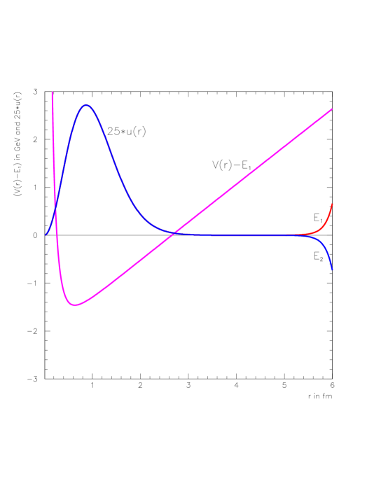
FIG. 1.: Here the $V_{q\bar{q}}$ potential has the quantum numbers of the $K_{J}$, $\ell_{\scriptscriptstyle u\bar{s}}=1$, and $s_{\scriptscriptstyle u\bar{s}}=1$. $(V_{q\bar{q}}(r)-E_{1})$ and $25\,u_{q\bar{q}}(r)$ are plotted for two solutions of equation (5), with trial energies $E_{1}=1.4299235012$ GeV and $E_{2}=1.4299235014$ GeV. The actual eigenenergy lies between these values. We plot $(V_{q\bar{q}}(r)-E_{1})$ rather than $V_{q\bar{q}}(r)$ so that the zero of $u(r)$ and the zero of available kinetic energy both lie on the $r$ axis. We pick the wavefunction normalization of 25 simply so we can see the wavefunction and the potential together.

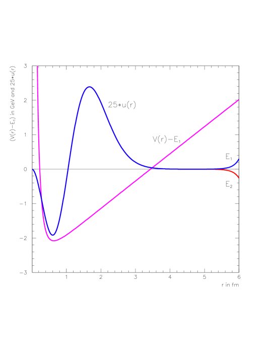
FIG. 2.: The same as FIG. 1., but for the first radially excited $K_{J}$ state. The trial energies are $E_{1}=2.047471763$ GeV and $E_{2}=2.047471768$ GeV.

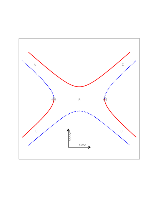
FIG. 3.: A quark line diagram for $s$–channel meson resonance formation in meson–meson scattering. The solid lines are quarks, the dashed lines are anti-quarks, and the shaded dots are ${q\bar{q}}$ annihilation or creation vertecies. Understanding the properties of the resonance $R$ in terms of the underlying ${q\bar{q}}$ interactions and the $AB\to R\to CD$ couplings is a goal of modern particle physics. As the lifetime of $R$ is typically $O(10^{-23})$ seconds it is clear that the properties of $R$ may depend significantly on its couplings to $AB$ and $CD$.

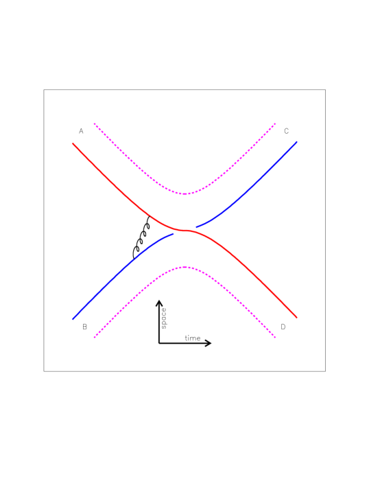
FIG. 4.: A quark line diagram for one–gluon exchange (the curly line) followed by quark exchange in meson–meson scattering. This diagram leads to non–resonant hadronic range van der Waals type intermeson potentials which have gaussian shapes and ranges of about 0.5 fm.

FIG. 5.: The relation between ${r_{{\scriptscriptstyle\!AB}}}$ and $r_{\scriptscriptstyle\!R}={r_{{q\bar{q}}}}$. Here $A=q_{1}\bar{q}_{3}$, $B=q_{2}\bar{q}_{4}$, and $R=q_{1}\bar{q}_{4}$. Clearly $r_{\scriptscriptstyle\!R}=2\,{r_{{\scriptscriptstyle\!AB}}}$ when all quarks are of equal mass.

FIG. 6.: Compare $\sin^{2}(\delta^{{\scriptscriptstyle\!BW}}_{{\scriptscriptstyle K\pi}})$ (the dots) and $\sin^{2}(\delta^{\scriptscriptstyle 2ch}_{{\scriptscriptstyle K\pi}})$ (the solid line) for $s$–wave $K\pi$ scattering. Here $\delta^{{\scriptscriptstyle\!BW}}_{{\scriptscriptstyle K\pi}}$ is the Breit–Wigner phase shift and $\delta^{\scriptscriptstyle 2ch}_{{\scriptscriptstyle K\pi}}$ (the solid line) is the phase shift found from the two–channel quark model, with the quark exchange potential in the quark model equal set to zero. The agreement between the two descriptions is excellent.

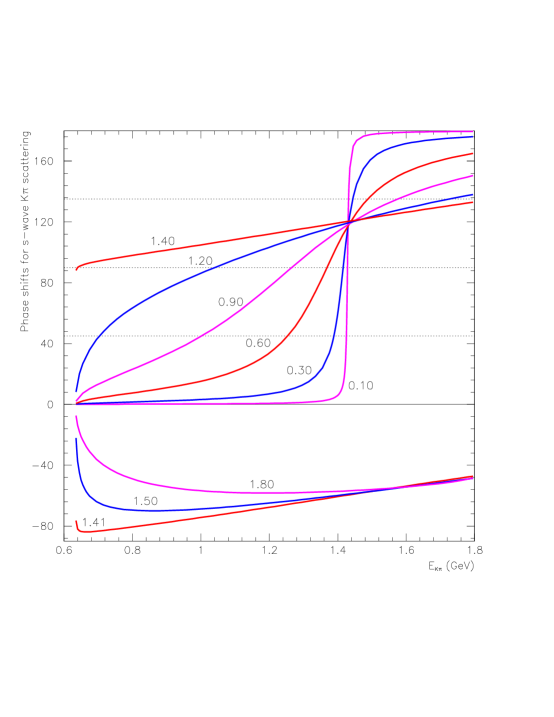
FIG. 7.: The variation in the 2–channel $K\pi$ $s$–wave scattering phase shift $\delta^{2ch}$ as $g$ varies. The horizontal dotted lines mark $45^{\circ}$, $90^{\circ}$, and $135^{\circ}$, and the numbers closest to the phase shifts give the value of $g$ in GeV. Note the departure from the Breit–Wigner phase shift description as the width increases, and the onset of a $K\pi$ bound state as $g$ grows larger than 1.40 GeV. We define the width as the energy difference between the energy at $\delta^{2ch}=135^{\circ}$ and $\delta^{2ch}=45^{\circ}$, and the resonance energy as the energy at which $\delta^{2ch}=90^{\circ}$.

FIG. 8.: $\sin^{2}(\delta^{\scriptscriptstyle 2ch}_{{\scriptscriptstyle K\pi}})$, from $s$–wave $K\pi$ scattering, is plotted from threshold to $E_{K\pi}=3.0$ GeV, with $g=0.60$ GeV and $\Gamma^{2ch}_{K_{0}}=280$ MeV. The peaks at 1.356, 2.020, and 2.553 GeV correspond to the ground state, the first radial excitation, and the second radial excitation of the $L=1$, $S=1$, $J=0$ strangeness $\pm 1$ resonance. The narrowing of the excited states depends on the form of the ${q\bar{q}}$ annihilation/creation verticies and requires further study. Note that heavier states have more open channels, and that here we are looking only at the partial width into a single channel.

FIG. 9.: The probability, $\int_{0}^{\infty}|u_{K_{\scriptscriptstyle 0}}^{\ast}u_{K_{\scriptscriptstyle 0}}|^{2}\,dr$, that the $s$-wave $K\pi$ scattering state is in a central ${q\bar{q}}$ resonance with $K_{\scriptscriptstyle 0}$ quantum numbers, plotted as a function of the $K\pi$ scattering energy. Note that some $u\bar{s}$ is always present in the central region. The location and widths of these peaks are directly related to the mass and width of the ${q\bar{q}}$ resonances.

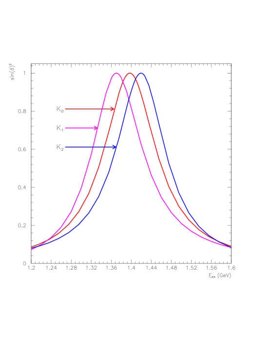
FIG. 10.: Resonance masses of the strangeness $\pm 1$ $\ell_{q\bar{q}}=1$, $s_{q\bar{q}}=1$, $J=0,1,2$ triplet as $J$ varies. The $K_{0}$ and $K_{2}$ are obtained from the $s$– and $d$–wave scattering of a $K\pi$ system respectively, while the $K_{1}$ is obtained from $s$–wave scattering of a $K^{\ast}\pi$ pair. The resonances masses are 1.397, 1.370, and 1.419 GeV for $J=0$, 1, and 2 respectively. The $K_{2}-K_{0}$ mass splitting of 22 MeV arises from the different vertex couplings to $K\pi$ whereas the $K_{0}-K_{1}$ mass difference of 17 MeV arises from $s$–wave couplings to different final states. The underlying $K_{0},\ K_{1},\ K_{2}$ masses, in this version of the naïve quark model are degenerate since we have omitted spin–orbit couplings in the Hamiltonian. The strength of the vertex couplings have been adjusted so each resonance has the same width in order to reduce the number of differences and clarify the discussion.

FIG. 11.: The dependence of the Breit–Wigner mass as extracted from the two–channel solution for $K\pi\leftrightarrow K_{0}$ scattering. The dots indicate the resonance masses for the ground, first radial, and second radial states. There is a third radial excitation just above 3.0 GeV.

FIG. 12.: The dependence of the Breit–Wigner width as extracted from the two–channel solution for $K\pi\leftrightarrow K_{0}$ scattering. The dots indicate the width predictions at the resonance energies for the ground, first radially excited, and second radially excited states. The location of the dots below the peaks indicates that the resonances are narrower on the low side than on the high side. The details of these results will change as more realistic models for the annihilation potentials are used.

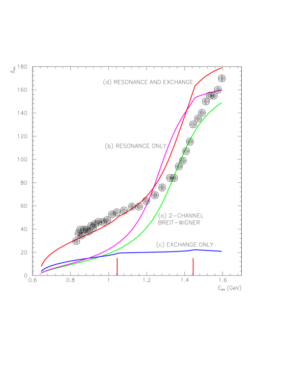
FIG. 13.: The $K\pi$ phase shift from the four–channel equation. (a) uses only $K\pi\leftrightarrow K_{0}$ couplings with no quark exchange potentials (so it’s just the Breit–Wigner phase shift), (b) uses only the resonance couplings of the three two–meson states to the $K_{0}$, (c) uses only quark exchange potentials, and (d) uses both quark exchange and resonance couplings. The data is from LASS [20]. The two vertical bars denote the onset of the $K\eta$ threshold at 1.045 GeV and the $K\eta^{\prime}$ threshold at 1.445 GeV. See Section VI for a discussion of these solutions.

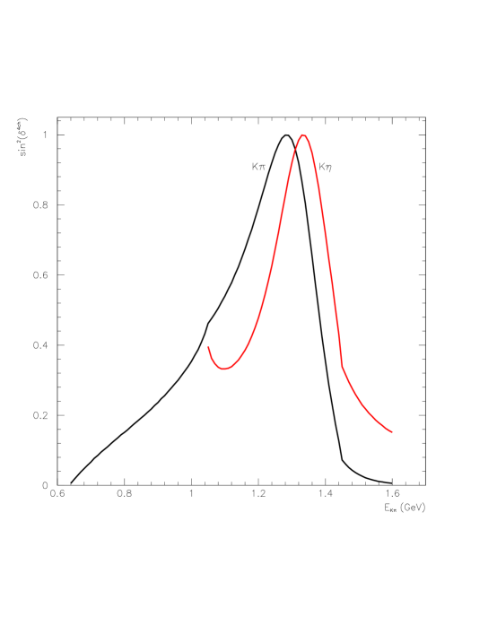
FIG. 14.: We plot $\sin^{2}(\delta^{4ch}_{K\pi\to K\pi})$ and $\sin^{2}(\delta^{4ch}_{K\pi\to K\eta})$ for the scattering processes $K\pi\to$ $(K\pi\leftrightarrow K\eta\leftrightarrow K\eta^{\prime}\leftrightarrow K_{0})\to K\pi$ and $K\pi\to$ $(K\pi\leftrightarrow K\eta\leftrightarrow K\eta^{\prime}\leftrightarrow K_{0})$ $\to K\eta$ where the curves are labelled by their final states. The 45 MeV mass difference in the central $K_{0}$ resonance in these two reactions is a pure multichannel effect. The decrease in $\sin^{2}(\delta^{4ch}_{K\pi\to K\eta})$ at $K\eta$ threshold suggests that there is a large $K\eta$ bound state component in the multichannel system below this energy. We use both $s$–channel resonance couplings and $t$-channel quark exchange to generate these curves.