Quasi-gaussian fixed points and factorial cumulants in nuclear multifragmentation

Abstract

We re-analyze the conditions for the phenomenon of intermittency (self-similar fluctuations) to occur in models of multifragmentation. Analyzing two different mechanisms, the bond-percolation and the ERW (Elattari, Richert and Wagner) statistical fragmentation models, we point out a common quasi-gaussian shape of the total multiplicity distribution in the critical range. The fixed-point property is also observed for the multiplicity of the second bin. Fluctuations are studied using scaled factorial cumulants instead of scaled factorial moments. The second-order cumulant displays the intermittency signal while higher order cumulants are equal to zero, revealing a large information redundancy in scaled factorial moments. A practical criterion is proposed to identify the gaussian feature of light-fragment production, distinguishing between a self-similarity mechanism (ERW) and the superposition of independent sources (percolation).

DAPNIA/SPhN-96-17, SPhT T96/067
Pacs: 24.60.Ky 25.70.Pq

1. Two classes of multifragmentation mechanisms: percolation and ERW models

In heavy-ion collisions, it is known that heavy excited systems are created and break into many lighter fragments of different sizes. This phenomenon is called multifragmentation. It occurs when the energy deposited in the system is sufficient to develop instabilities but not enough to totally evaporate the system into nucleons. A statistical analysis of the average spectrum is consistent with a power-law dependence of the fragment-size distribution. Some interesting interpretations of multifragmentation based on a phase transition in nuclear matter have been motivated by the experimental form of the fragment-size distribution[1, 2], compatible with a power-law. Indeed, several critical phenomena, such as for instance percolation and liquid-gas phase transition exhibit a similar power-law of the fragment-size distribution at the critical point[3, 4]. In these systems, the rôle of fragments is played by connected clusters of a given phase inside the other phase and the size distribution of clusters is proven to take the general form:

$$N(s,\varepsilon)\sim s^{-\tau}\!\cdot f(s\ {\varepsilon}^{\sigma})\hskip 85.35826pt\tau,\sigma>0,$$ (1)

where $s$ is the cluster size and $\varepsilon$ characterizes the distance from the critical point. In a thermal phase transition $\varepsilon=T-T_{c}$ with $T_{c}$ the critical temperature. In a bond-percolation model $\varepsilon$ = $r_{c}-r$, with $r$ the probability for the bond between two neighbouring sites to be broken and $r_{c}$ its critical value. The genuine phase transition is well-known to only occur when the system is infinite. However finite systems show specific features related to the continuous limit, including finite-size corrections[3, 4]. In multifragmenting systems, the parameter $\varepsilon$ is not well identified. It could be associated with the excitation energy deposited into the system by the collision.

One typical property of phase transitions is the existence of large, scale invariant fluctuations near the critical point[3]. In order to extract a signal from fluctuation patterns, one has proposed[5] in nuclear physics a method based on factorial moments. This method was originally designed[6] for the rapidity spectra of ultra-relativistic multiparticle production but can be extended to other problems. Dividing the phase space into $M$ bins of size $\delta$, the factorial moment of order $p$ can be defined by

$$F_{p}(\delta)=\frac{\sum_{s=1}^{M}{<\!n_{s}(n_{s}-1)\cdots(n_{s}-p+1)\!>}}{\sum_{s=1}^{M}{{<\!n_{s}\!>}^{p}}},$$ (2)

where $n_{s}$ is the number of ”objects” in the $s^{th}$ bin and the average is taken over the set of events. In high-energy physics, ”Objects” are particles distributed as a function of the rapidity variable. In nuclear physics, they are fragments distributed as a function of the size.

In particle physics, the interest of factorial moments has been to deconvolute the statistical fluctuations due to the limited number of ”objects” observed by event. It has revealed the existence of self-similar fluctuations, called intermittency, that is:

$$F_{p}(\delta)\propto{\delta}^{-\alpha_{p}},$$ (3)

where $\alpha_{p}$ is the so-called intermittency exponent. For event-by-event fluctuations of multifragmentation spectra[5], one considers $M$ bins of size $\delta$=$\frac{A}{M}$ along the fragment-size axis ($A$ being the mass of the excited system). When $M$ is varied, a behaviour like (3) was observed in the fragment-size distribution of ${}^{197}_{79}$Au₁₁₈ nucleus multifragmenting in a nuclear emulsion[7]. The signal was compared with that obtained from a site-bond percolation model in a network of size 6³, showing a similar behaviour at the critical point. The behaviour (3) was thus interpreted as a phase-transition signal.

However the application of the method to the fragment-size distribution is less straightforward than for rapidity spectra of particles. Indeed, the expression (2) is dominated by the first bin, i.e. the one containing the lightest fragments. In particular, no fragment of mass greater than $A/p$ can contribute to $F_{p}$. This introduces an important bias in the analysis, and has to be properly taken into account.

On a less technical ground, several remarks have made the phase-transition interpretations doubtful[8]. In percolation models, the signal disappears when the size of the system goes to infinity. Moreover, $F_{p}(\delta)$ seems to strongly depend on the shape of the total multiplicity distribution. In particular, when selecting events with the same multiplicity, the signal disappears.

The interpretation is made more puzzling when considering a different class of multifragmentation mechanisms which leads to an intermittency behaviour without relying on a phase transition: the ERW model[9]. Though there is no quantitative multifragmentation model using this mechanism, its simplicity has made it a fruitful toy model for understanding the mechanisms behind intermittency. In this case, the rule is to create fragments of different sizes with a Monte-Carlo procedure as follows. The average fragment-size distribution is constrained to be a power-law distribution $P(s)$ $\sim$ $s^{-\tau}$, $\tau$ being a parameter of the model. We note $A$ the total mass. An event is specified by a set of random numbers $\eta_{1},\eta_{2},\cdots,\eta_{n}$ (with $0\leq\eta_{i}\leq 1$), which defines a set of successive binary fragmentations (see Fig. 1). $\eta_{1}$ defines a first fragmentation into two fragments of mass $a_{1}$ and $A-a_{1}$, where $a_{1}$, an inert fragment present in the final event, is implicitely defined by

$$\frac{\sum_{s=1}^{a_{1}-1}{s^{-\tau}}}{\sum_{s=1}^{A}{s^{-\tau}}}<\eta_{1}\leq\frac{\sum_{s=1}^{a_{1}}{s^{-\tau}}}{\sum_{s=1}^{A}{s^{-\tau}}}.$$ (4)

The event is completed by repeating the operation with the mass $A-a_{1}$ (or $A-\sum_{i=1}^{k}{a_{i}}$ after $k$ generations) until the total mass is exhausted. This model has many interesting properties[9], in particular, an intermittent signal can be seen for $1.8<\tau<2.0$.

Using the two different classes of mechanisms, percolation and ERW models we will re-examine the problem of interpreting intermittency by asking the following questions:

(i) Is there a common scale-invariant mechanism behind the different realisations of intermittency?

(ii) Are there statistical tools which could be more suitable than factorial moments for the study of multifragmentation spectra?

(iii) Can we distinguish between different mechanisms?

The plan of our study is as follows. In section 2, we show in both models the existence of fixed points, where the shape of the multiplicity is stable when the size of the system goes to infinity. This shape is quasi-gaussian for the total multiplicity and bin-size invariant but not gaussian when selecting the second bin. In section 3, we show that factorial cumulants[11], instead of moments, are best suitable for the study of gaussian fluctuations of the multiplicity spectra. In the final section, we propose a criterion to distinguish between models, together with a physical interpretation of the different mechanisms in action.

2. Quasi-gaussian fixed points

Let us introduce well-known coefficients which characterize the shape of a statistical distribution. For a given variable $m$, these are defined by

$$\gamma_{i}=\frac{<{(m-<m>)}^{(i+2)}>}{{<(m-<m>)^{2}>}^{(\frac{i+2}{2})}}$$ (5)

In particular, we will consider the skewness ($\gamma_{1}$) and sharpness ($\gamma_{2}$) coefficients. For a gaussian probability distribution $\gamma_{1}=0$ and $\gamma_{2}=3$. The number $\gamma_{1}$ (resp. $\gamma_{2}$) describes the main assymetric (resp. symetric) variation with respect to the gaussian. Interestingly enough, we have found fixed points in the parameter space, where the values of $\gamma_{1}$, $\gamma_{2}$ evaluated for the total multiplicity nearly reach gaussian values. We call them quasi-gaussian fixed points.

We have performed a systematic analysis of the multiplicity distributions in the ERW (Fig. 2) and percolation (Fig. 3) models. Using ERW, we have first plotted the values taken by $\gamma_{1}$ and $\gamma_{2}$ for the total multiplicity distribution as a function of $\tau$ (see Fig. 2-a) for different values of $A$ ($50\leq A\leq 500$). Each of the points reported on these figures is calculated with statistics of about 10⁵ events. We note the existence of a value $\tau\sim 1.8$ where all curves intersect. Interestingly enough, this value is in the range where the intermittency behaviour has been noticed[9]. The values of $\gamma_{1}$ and $\gamma_{2}$ at the ”fixed point” are close respectively to $0$ and $3$ but nevertheless slightly different. The total multiplicity distribution is thus quasi-gaussian. We also note the existence of a minimum for $\gamma_{2}$ near $\tau$ $\sim$ $2$ which confirms that the intermittent signal occurs when fluctuations are maximal. This study has revealed the existence of a scale-invariant property of the total multiplicity distribution.

In order to understand its connection with the intermittency signal, an analysis at fixed total size but varying the bin size appears useful. We thus studied in more detail the multiplicity distribution in the second bin $n_{2}(\delta)$ (Fig. 2-b). The results are shown for $\gamma_{1}$ and $\gamma_{2}$ as a function of $\tau$. The curves correspond to varying values of the bin size ($4\leq\delta\leq 64$) with a fixed value of the system size $A=128$. There is again a clear evidence for a ”fixed point”. We have also verified that this fixed point remains when the system size increases. We note that the corresponding value of $\tau$ is similar but slightly different than that of Fig. 2-a. Nevertheless, it remains in the region where the intermittent behaviour is noticed. The same analysis for the first bin distribution $n_{1}(\delta)$ is not relevant because the values of $\gamma_{1}$ and $\gamma_{2}$ are strongly dominated by the distribution of fragments of mass one. In order to study the scale-invariance properties as a function of the bin size $\delta$, it is thus necessary to avoid as much as possible the statistical bias due to the dominance of mass-one fragments. Moreover, there could be good experimental reasons to avoid the contribution of lightest fragments[10] which can be contaminated by other processes than nuclear multifragmentation (e.g. pre-equilibrium, secondary emission, etc…).

The same analysis was performed with the finite-size bond percolation model (Fig. 3). One considers a 3-dimensional cubic lattice with a probability $r$ of breaking a bond. The critical value of the bond-breaking probability $r_{c}$ is around $0.76$ ($0.7512$ in the continuous limit[4]). We have first plotted the values of $\gamma_{1}$ and $\gamma_{2}$ for the total multiplicity distribution as a function of $r$ for various sizes of the system ($4^{3}\leq A\leq 10^{3}$), see Fig. 3-a. Each point corresponds to the same statistics ($10^{5}$ events) as for the previous study. There is evidence for a fixed point in $\gamma_{1}$ near $r_{c}$. The fixed-point behaviour is less clear for the sharpness parameter $\gamma_{2}$. The values of $\gamma_{1}$ and $\gamma_{2}$ remain respectively near $0$ and $3$ confirming the existence of a quasi-gaussian shape in the critical region of the parameter. In the same region, intermittency has been observed[5]. In the second bin, the analysis of $\gamma_{1}$ and $\gamma_{2}$ (Fig. 3-b) clearly indicates the existence of a fixed point in the same parameter range.

The strong similarities between the two models and the location of the fixed point in the same parameter region where intermittency occurs, calls for a deeper analysis of intermittency. Indeed, the quasi-gaussian features of the total multiplicity distribution require a specific treatment of intermittency which goes beyond the use of factorial moments.

3. Factorial cumulants

The existence of quasi-gaussian distributions leads us to introduce new statistical tools for multifragmentation, namely the factorial cumulants. In particle physics, they have been introduced[11] in order to combine the elimination of the statistical noise using the factorial form with the well-known property of cumulants. Cumulants are a-priori able to disentangle genuine higher-order correlations from combinations of lower-order correlations which appear in factorial moments. In particular, gaussian fluctuations are governed by 2-body correlations implying the vanishing of cumulants of order greater than two. Let us apply this tool to nuclear multifragmentation taking into account the specific normalisation used in formula (2). We first introduce the generating function of unscaled factorial moments

$$G(\lambda)=\sum_{s=1}^{M}{<\!\lambda^{n_{s}}\!>},$$ (6)

where $\lambda$ is an arbitrary parameter and the average $<\cdot>$ is performed over the set of events. For instance, formula (2) can be identically written as

$$F_{p}(\delta) = \left.\frac{\left(\frac{\partial^{p}G(\lambda)}{\partial\lambda^{p}}\right)}{\left(\frac{\partial G(\lambda)}{\partial\lambda}\right)^{p}}\right|_{\lambda=1}.$$ (7)

Using the logarithm of the generating function, the general expression of the scaled factorial cumulants can be written

$$K_{p}(\delta) = \left.\frac{\left(\frac{\partial^{p}\ln G(\lambda)}{\partial\lambda^{p}}\right)}{\left(\frac{\partial G(\lambda)}{\partial\lambda}\right)^{p}}\right|_{\lambda=1}.$$ (8)

For instance, the first cumulants read

$$K_{2}(\delta) = \frac{\sum_{s=1}^{M}{\left(<\!n_{s}(n_{s}-1)\!>-<\!n_{s}\!>^{2}\right)}}{\sum_{s=1}^{M}{<\!n_{s}\!>^{2}}},$$ (9)

$$K_{3}(\delta) = \frac{\sum_{s=1}^{M}{\left(<\!n_{s}(n_{s}-1)(n_{s}-2)\!>-3<\!n_{s}(n_{s}-1)\!><\!n_{s}\!>+2<\!n_{s}\!>^{3}\right)}}{\sum_{s=1}^{M}{<\!n_{s}\!>^{3}}},$$ (10)

$$K_{4}(\delta) = \frac{\sum_{s=1}^{M}{\left(<\!n_{s}(n_{s}-1)(n_{s}-2)(n_{s}-3)\!>-4<\!n_{s}(n_{s}-1)(n_{s}-2)\!><\!n_{s}\!>\right)}}{\sum_{s=1}^{M}{<\!n_{s}\!>^{4}}},$$ (11)

$$+ \frac{\sum_{s=1}^{M}{\left(-3<\!n_{s}(n_{s}-1)\!>^{2}+12<\!n_{s}(n_{s}-1)\!><\!n_{s}\!>^{2}-6<\!n_{s}\!>^{4}\right)}}{\sum_{s=1}^{M}{<\!n_{s}\!>^{4}}}.$$ (12)

It is interesting to note that the choice of normalisation (2) implies that the scaled factorial cumulants cannot in general be expressed as combinations of scaled factorial moments. If however, the first bin dominates the evaluation of moments, one obtains the following approximate relations:

$$K_{2}(\delta) \simeq F_{2}(\delta)-1,$$ (13)

$$K_{3}(\delta) \simeq F_{3}(\delta)-3\cdot F_{2}(\delta)+2,$$ (14)

$$K_{4}(\delta) \simeq F_{4}(\delta)-4\cdot F_{3}(\delta)-3\cdot{(F_{2}(\delta))}^{2}+12\cdot F_{2}(\delta)-6.$$ (15)

Note that the direct determination of cumulants using formula (8) could be useful to avoid the errors on the combinations of factorial moments.

Let us apply our formalism to the ERW and percolation models. We have first computed the factorial moments using definition (1), see Fig. 4-a and 4-b. The result obtained with the ERW model is displayed in Fig 4-a with a total mass $A=128$ using the critical value $\tau=1.8$. The figure 4-b corresponds to the same observables for the bond-percolation model with $A=6^{3}$ and $r\simeq 0.75=r_{c}$. The curves reproduce (for slightly different parameter values) the results of refs.[5] and [9]. Note that, for completion, we have also reported the ERW factorial moments for the value $\tau=2.3$ corresponding to the slope observed in the critical region of the bond-percolation model. The results exhibit a nearly linear increase as a function of the bin size which is typical of an intermittent behaviour.

We have calculated the factorial cumulants corresponding to formula (9) for the ERW (Fig. 4-c) and percolation (Fig. 4-d) models. Cleary, only the second cumulant $K_{2}(\delta)$ is significantly different from 0. The higher order factorial cumulants are nearly zero for all bin size $\delta$. Note that due to the smallness and the change of sign of cumulants, it is not convenient to plot their logarithm. Indeed, the cumulants obtained for both models correspond to strong cancellations between the large and positive scaled factorial moments. This confirms that there is a redundancy of information in factorial moments which is solved by using cumulants.

The figures 4-c and 4-d show a clear indication of a rise of $K_{2}(\delta)$ especially for the percolation model. When compared to Fig. 5, where scaled factorial cumulants are displayed for the bond-percolation model outside the critical region, the behaviour of $K_{2}(\delta)$ is revealing intermittent fluctuations. Indeed, an intermittent singularity in factorial moments should also appear in the second cumulant since it cannot be absorbed by the lower order contributions. For small values of $K_{2}(\delta)$ the first relation (10) gives

$$K_{2}(\delta)\ \simeq\ \log(F_{2}(\delta))\ \propto\ -\alpha_{p}\ \log(\delta).$$ (16)

Such a behaviour is observed in Fig. 4. It is interesting to note that the dominance of second-order cumulants is valid for all values of the parameter $r$ in the percolation model.

Considering the abovementionned properties of scaled factorial cumulants for multifragmentation mechanisms, a series of comments are in order:

(i) The scaled factorial moments of multifragmentation models seem to contain redundant information, since only the second cumulant is significantly different from zero. In the framework of the approximation (10), which is valid since the first bin is largely dominating, it means that the scaled factorial moments can all be expressed as functions of $K_{2}(\delta)$.

(ii) In the percolation model, the cumulant analysis indicates that the same property still holds outside the critical region, see Fig. 5. However, it is only around the critical region $r\sim 0.75$ that one observes a rise of $K_{2}(\delta)$ specific of intermittency.

(iii) A qualitative difference exists between the behaviour of $K_{2}(\delta)$ for the ERW and the percolation models. They take very different values for the largest bin size ($\delta\equiv A$), i.e. the second cumulants of the total multiplicity distributions are significantly different.

(iv) We also remarked that the slope of $K_{2}(\delta)$ decreases with increasing system size, similarly to what has been observed for scaled factorial moments[8]. However, the order-of-magnitude difference still remains between the values of $K_{2}(\delta)$ for the ERW and the percolation models.

4. Discussion and summary of results

Our analysis of multifragmentation spectra using the comparison of two generic mechanisms, ERW and percolation, calls for a physical interpretation. The existence of a scaling behaviour for the profile parameters $\gamma_{1}$, $\gamma_{2}$, being a common feature of both models in their respective critical regime, points to the existence of a scale-invariant property of multiplicity distributions. It is phenomenologically clear that this ”fixed-point” is related to the intermittency signal and thus to a certain type of criticality of the system. The criticality is explicit for percolation, since it corresponds to a phase transition in the continuous limit, but is hidden in the formulation of the ERW mechanism.

Observing at the same time a quasi-gaussian shape of the total multiplicity and a large dominance of $K_{2}(\delta)$ over higher order cumulants unravels a pronounced gaussian feature of multifragmentation mechanisms when small-mass fragments dominate the observables. Two main interpretations may naturally explain these features. It may come either from the existence of a self-similar fragmentation mechanism with a scale invariant gaussian fixed-point or from the superposition of many independent sources of fragments leading to a gaussian distribution through the central-limit theorem. As we once more want to stress, the gaussian property is mainly inherent to the production of lighter elements.

In order to distinguish between the two options, let us study the two parameters which define a gaussian distribution namely the distribution average $<m>$ and its variance $\sigma=<(m-<m>)^{2}>$. One expects[12] $\sigma/\!<\!n\!>\rightarrow cste$ for self-similar models and $\sigma/\!<\!n\!>$ $\propto$ $1/\!\sqrt{<\!n\!>}$ for the independent sources. Indeed, in this latter case the number of independent sources is expected to grow with the multiplicity. Then the central-limit theorem gives the quoted prediction for $\sigma/\!<\!n\!>$. In Fig. 6, we display the quantity $\sigma/\!<\!n\!>$ for each model for both the total multiplicity distribution and the mass-one fragment distribution. For the total multiplicity, power-law fits give $\sigma/\!<\!n\!>$ $\propto$ ${<\!n\!>}^{-0.01}$ for the ERW model and $\sigma/\!<\!n\!>$ $\propto$ ${<\!n\!>}^{-0.44}$ for the percolation model. Interestingly enough, the fits are very similar for the mass-one fragments with a power dependance ${<\!n\!>}^{-0.49}$ for the percolation model very suggestive of a central-limit signature. Hence, the ERW is a self-similar mechanism, while percolation is gaussian with a central-limit type for the production of light fragments.

Let us summarize our main results by proposing the following new tools of analysis for multifragmentation fragment distributions.

(i) The shape parameters $\gamma_{1}$, $\gamma_{2}$ for the total multiplicity and for the second-bin multiplicity can be studied as a function of the system size, and for the second case as a function of the bin size. We expect a fixed-point behaviour for the critical region of multifragmentation. Intermittency is expected to occur in the same region. Note that the second bin could be experimentally easier to study, since it avoids the ambiguity on the origin of lightest fragments and can be used at fixed total-size by varying only the bin-size.

(ii) The study of fluctuations using scaled factorial moments suffers from a large redundancy of information. For the class of models under study, we suggest using instead the scaled factorial cumulants of fluctuations.

(iii) The gaussian feature of the light-fragment distributions revealed both by the quasi-gaussian fixed point property and the scaled factorial cumulants is an important characteristics to be studied in nuclear multifragmentation. Note that this gaussian feature has also been noticed in a different model[13], confirming the interest of studying this property in detail. Two mechanisms seem to give an alternative for explaining the gaussian features, namely either a self-similar fixed-point or a superposition of independent emission sources for light fragments. They can be distinguished by dependence of $\sigma/\!<\!n\!>$ with $<\!n\!>$ or equivalently by the factorial cumulants for large bins. As an application, we found that the ERW model is self-similar while percolation probably leads to independent sources for the production of light fragments even outside the critical region. We expect the self-similar property to be shared by models based on a tree structure of multifragmentation[14, 15]. In the same spirit we also expect models based on second-order phase transitions to follow the same trend governed by the central-limit theorem as the percolation model for the distribution of light fragments.

ACKNOWLEDGMENTS

The authors thank Roland Dayras and Jean-Louis Meunier for many fruitful discussions and Bertrand Giraud for a careful critical reading of the manuscript. One of us (D.L.) thanks the SPHN for its hospitality and physicists for their kindness.

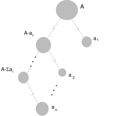
FIG. 1.: Event generation in the ERW model. The set of successive fragments $a_{1},a_{2}\cdots,a_{n}$ is defined by the set of random number $\eta_{1},\eta_{2},\cdots,\eta_{n}$ (see formula (4)). The generation of random numbers is stopped when $\sum_{i=1}^{n}{a_{i}}>A$.

FIG. 2.: Shape parameters $\gamma_{1}$, $\gamma_{2}$ of the multiplicity distributions for the ERW model.
a) Top: $\gamma_{1}$, $\gamma_{2}$ (total multiplicity distribution) as a function of $\tau$ for different system sizes ($A=50,100,200,300,400$ and $500$). b) Bottom: $\gamma_{1}$, $\gamma_{2}$ (second bin) as a function of $\tau$ for different values of the bin size $\delta$ ($A=128$).

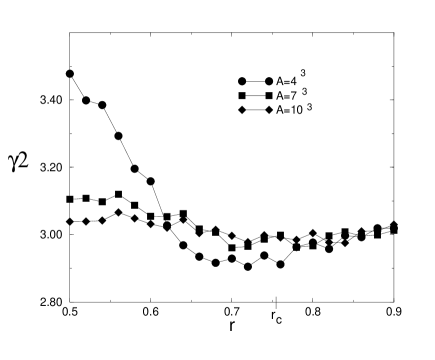
FIG. 3.: Shape parameters $\gamma_{1}$, $\gamma_{2}$ for multiplicity distributions for the bond-percolation model. a) Top: $\gamma_{1}$, $\gamma_{2}$ (total multiplicity distribution) as a function of $r$ for different system sizes $A$. b) Bottom: $\gamma_{1}$, $\gamma_{2}$ (second bin) as a function of $r$ for different values of the bin size $\delta$ ($A=6^{3}$).

$log(F_{p}(\delta))$		$log(F_{p}(\delta))$

$K_{p}(\delta)$		$K_{p}(\delta)$

FIG. 4.: Scaled factorial moments $F_{p}(\delta)$ and cumulants $K_{p}(\delta)$. a) $\log(F_{p}(\delta))$ as a function of $-\log(\delta)$ in the ERW model for $A=128$, $\tau=1.8$ (solid line) and $\tau=2.3$ (dashed line). b) $\log(F_{p}(\delta))$ as a function of $-\log(\delta)$ in the percolation model for $A=6^{3}$ and $r=0.75$. c) $K_{p}(\delta)$ vs $-\log(\delta)$ in the ERW model for $A=128$ and $\tau=1.8$ (solid line) and $\tau=2.3$ (dashed line). d) $K_{p}(\delta)$ vs $-\log(\delta)$ in the percolation model for $A=6^{3}$ and $r=0.75$.

$K_{p}(\delta)$		$K_{p}(\delta)$

FIG. 5.: Scaled factorial cumulants $K_{p}(\delta)$ outside the critical region for the bond-percolation model. a) $K_{p}(\delta)$ as a function of $\delta$ for $r=0.90$ and $A=6^{3}$. b) $K_{p}(\delta)$ for $r=0.60$ and $A=6^{3}$.

FIG. 6.: The scaled variance $\sigma/\!<\!n\!>$ as a function of $<\!n\!>$. $\sigma/\!<\!n\!>$ is displayed as a function of the average multiplicity. Circles correpond to the variance and average of the total multiplicity distribution; stars correspond to the variance and average multiplicity distribution of mass-one fragments. For the ERW model with $\tau=1.8$, each point corresponds to a given total mass $A$ taken in the intervalle [100,10000]. Power-law fits are displayed by continuous lines, the powers are $-0.01$ (circles) and $-0.06$ (stars) in the ERW case. For the bond-percolation model, $r=0.76$ and each point corresponds to a fixed value of $A$ ($A=3^{3},4^{3},\cdots,20^{3}$). The power-law fits are found respectively equal to $-0.44$ (circles) and $-0.49$ (stars).

REFERENCES

-
[1]
X. Campi, J. Phys. A19 (1986) L917.
J. Desbois, Nucl. Phys. A466 (1987) 724.
X. Campi, Phys. Lett. B208 (1988) 351.
See also W. Bauer, D.R. Dean, U. Mosel and U. Post, Phys. Lett. B150 (1985) 53. -
[2]
J. Randrup and S.E. Koonin, Nucl. Phys. A356 (1981) 223.
D. H. E. Gross, Nucl. Phys. A428 (1984) 313c. - [3] H.E. Stanley, Phase transitions and critical phenomena, (Oxford University Press Ed., 1971).
- [4] D. Stauffer and A. Aharony, Introduction to percolation theory, (London: Taylor & Francis 2nd Edition 1992).
- [5] M. Ploszajcak and A. Tucholski, Phys. Rev. Lett. 65 (1990) 1539; Nucl. Phys. A523 (1995) 651.
- [6] A. Bialas and R. Peschanski, Nucl. Phys. B273 (1986) 703; B308 (1988) 857.
- [7] C. J. Waddington and P.S. Freier, Phys. Rev. C31 (1985) 888.
- [8] X. Campi and H. Krivine, Nucl. Phys. A589 (1991) 505.
- [9] B. Elattari, J. Richert and P. Wagner, Nucl. Phys. A560 (1993) 603.
- [10] M. L. Cherry et al., Phys. Rev. C53 (1995) 1532.
-
[11]
A.H. Mueller, Phys. Rev. D4 (1971) 150.
P. Carruthers, H. C. Eggers and I. Sarcevic, Phys. Lett. B254 (1991) 258.
P. Lipa, H.C. Eggers and B. Buschbeck, Phys. Rev. D53 (1996) 4711.
For definitions and references, see E.A. De Wolf, I.M. Dremin, W. Kittel, Phys. Rep. 270 (1996) 1. - [12] We thank J.-L. Meunier for suggesting this criterion.
- [13] A. R. DeAngelis, D.H.E. Gross and R. Heck, Nucl. Phys. A537 (1992) 606.
- [14] B.G. Giraud, R. Peschanski, Phys. Lett. B315 (1993) 452; B343 (1995) 415. B.G. Giraud, R. Peschanski, Wei-hsing Ma, Phys. Rev. E52 (1995) R4599.
- [15] R. Botet and M. Ploszajczak, Phys. Rev. Lett. 69 (1992) 3696; Preprint GANIL P 96 07 (1996), for recent review and references.