A Non-Perturbative Treatment of the Pion in the Linear Sigma-Model
Z. Aouissat⁽¹⁾, G. Chanfray⁽²⁾, P. Schuck⁽³⁾ and J. Wambach⁽¹⁾,

⁽¹⁾ Institut für Kernphysik, Technische Hochschule Darmstadt, Schloßgartenstraße 9, D-64289 Darmstadt, Germany.
⁽²⁾ IPN-Lyon, 43 Bd. du 11 Novembre 1918, F-69622 Villeurbanne Cédex, France.
⁽³⁾ ISN, 53 avenue des Martyrs, F-38026 Grenoble Cédex, France.

Using a non-perturbative method based on the selfconsistent Quasi-particle Random-Phase Approximation (QRPA) we describe the properties of the pion in the linear $\sigma$-model. It is found that the pion is massless in the chiral limit, both at zero- and finite temperature, in accordance with Goldstone’s theorem.

1 Introduction

Chiral Lagrangians, as the effective low-energy realization of QCD, have become increasingly important in hadronic physics. In the sector of up and down quarks and for vanishing quark masses, QCD exhibits an exact global $SU(2)_{L}\times SU(2)_{R}$ chiral symmetry. In the non-perturbative vacuum, this symmetry is spontaneously broken to its vectorial subgroup $SU(2)_{V}$ with the appearence of pions as Goldstone bosons. The interaction of the Goldstone bosons is greatly restricted by chiral symmetry involving the ratios $(m_{\pi}/4\pi f_{\pi})^{2}$ and $(E_{\pi}/4\pi f_{\pi})^{2}$ as a small expansion parameters, where $m_{\pi}$, $E_{\pi}$ and $f_{\pi}$ denote the pion mass, the pion energy and the weak pion decay constant respectively. A systematic expansion is provided by chiral perturbation theory [1]. For example, the $\pi-\pi$ scattering amplitude is determined order by order in the number of derivatives. In this way the low-energy theorems are known to be maintained. For many reasons, however, it would be interesting to have a non-perturbative approach while still maintaining the low-energy theorems. One obvious reason is the requirement of unitarity of the S-matrix in the scattering problem. Another relates to the thermodynamics of effective chiral theories, especially in the study of chiral restauration. As the critical point is approached one cannot expect perturbation theory to provide a valid description.

Needless to say that the question of preserving the symmetries non-perturbatively is a very delicate one [2]. While in perturbative calculations the class of diagrams that ought to be considered in order to preserve the symmetries in the physical observables is well known, the situation is far less clear in the non-perturbative case. The aim of the present paper is to demonstrate that such a program is indeed possible. Our theoretical framework will be the linear $\sigma$-model which is especially suited for the techniques to be employed. These techniques have their origin in many-body physics and consist of a mean-field treatment via a Bogoliubov rotation supplemented by RPA fluctuations. It is well known that such an approach, while being non-perturbative, treats symmetries and spontaneous symmetry breaking correctly [3]. We shall demonstrate that, exactly as in the fermionic case, the RPA built on the selfconsistent mean field is able to restore the symmetry broken by the mean-field vacuum.

The paper is organized as follows: First the formulation of the bosonic mean-field problem will be given in sect. 2. In the ’quasi-particle basis’ thus obtained, the RPA excitation spectrum for the single-pion mode is constructed in sect. 3. It will be shown explicitly that this spectrum contains a zero mode in the chiral limit, to be identified with the ’Goldstone pion’. In sect. 4 the formalism will be extended to finite temperature as a first step towards a non-pertubative description of the chiral phase transition. Again, there is no mass generation in the chiral limit. Conclusions and an outlook are given in sect. 5.

2 The Bogoliubov Rotation

The starting point is the Lagrangian density of the linear $\sigma$-model [4]

$${\cal L}=\frac{1}{2}\left[\left(\partial_{\mu}{\bf{\pi}}\right)^{2}+\left(\partial_{\mu}{\hat{\sigma}}\right)^{2}\right]-\frac{\mu_{0}^{2}}{2}\left[{\bf{\pi}}^{2}+{\hat{\sigma}}^{2}\right]-\frac{\lambda_{0}^{2}}{4}\left[{\bf{\pi}}^{2}+{\hat{\sigma}}^{2}\right]^{2}+c{\hat{\sigma}}.$$ (1)

where $\lambda_{0}$ represents the bare coupling constant, $\mu_{0}$ the mass parameter and $\pi$ and ${\hat{\sigma}}$ denote the bare pion and sigma fields, respectively. Chiral symmetry is explicitly broken (in the PCAC sense) by the last term in the Lagrangian, $c{\hat{\sigma}}$. At tree level the pion and sigma masses are given by

$$m_{\pi}^{2} = \mu_{0}^{2}+\lambda_{0}^{2}\langle{\hat{\sigma}}\rangle^{2}$$

$$m_{\sigma}^{2} = \mu_{0}^{2}+3\lambda_{0}^{2}\langle{\hat{\sigma}}\rangle^{2}$$

$$c = \langle{\hat{\sigma}}\rangle\mu_{0}^{2}+\lambda_{0}^{2}\langle{\hat{\sigma}}\rangle^{3}$$ (2)

The pion possesses manifestly the Goldstone boson character since its mass is trivially proportional to $c$. The perturbative one loop calculation preserves this result as is shown for instance in [5].
For further development it is now convenient to define the field operators in terms of creation and annihilation operators as

$$\pi_{i}({\bf x}) = \int\frac{d^{3}{\bf q}}{\sqrt{(2\pi)^{3}2\omega_{q}}}\left(a_{{\bf q}\,i}e^{i{\bf q}{\bf x}}+a^{+}_{{\bf q}\,i}e^{-i{\bf q}{\bf x}}\right)$$

$${\hat{\sigma}}({\bf x}) = \int\frac{d^{3}{\bf q}}{\sqrt{(2\pi)^{3}2\omega_{q}}}\left(b_{{\bf q}}e^{i{\bf q}{\bf x}}+b^{+}_{{\bf q}}e^{-i{\bf q}{\bf x}}\right)$$ (3)

where the frequency $\omega_{q}$, common to both fields, is given by

$$\omega_{q}=\sqrt{\mu_{0}^{2}+q^{2}}.$$ (4)

In a first step a canonical transformation is performed for the pion as well as the sigma field. Thus we introduce a new set of creation and annihilation operators through the following Bogoliubov rotation

$$\alpha^{+}_{q} = u_{q}a^{+}_{q}-v_{q}a_{q},$$

$$\beta^{+}_{q} = x_{q}b^{+}_{q}-y_{q}b_{q}-w_{q}$$ (5)

with $u_{q}$, $v_{q}$, $x_{q}$ and $y_{q}$ being even functions of their argument, and $w_{q}$ a c-number. The first equation is the usual bosonic Bogoliubov transformation applied to the pion field. The new vacuum with respect to these $\alpha_{q}$ operators is the well-known ’squeezed state’. In the second equation the transformation contains an additional ’shift’ $w_{q}$ to account for the macroscopic condensate $\langle{\hat{\sigma}}\rangle$. For later notation we will adopt the variable s to designate this condensate. To render the transformations canonical the Bogoliubov factors have to obey the following constraints

$$u_{q}^{2}-v_{q}^{2}=1,\quad\quad\quad x_{q}^{2}-y_{q}^{2}=1.$$ (6)

In the ’quasi-boson’ basis eq.(5) the fields and their conjugates read

$$\pi_{j}({\bf x}) = \int\frac{d^{3}{\bf q}}{\sqrt{(2\pi)^{3}2\omega_{q}}}\left(u_{q}+v_{q}\right)\left(\alpha_{q\,j}e^{i{\bf q}{\bf x}}+\alpha^{+}_{q\,j}e^{-i{\bf q}{\bf x}}\right)$$

$${\dot{\pi}}_{j}({\bf x}) = \int\frac{d^{3}{\bf q}}{\sqrt{(2\pi)^{3}2\omega_{q}}}(-i\omega_{q})\left(u_{q}-v_{q}\right)\left(\alpha_{q\,j}e^{i{\bf q}{\bf x}}-\alpha^{+}_{q\,j}e^{-i{\bf q}{\bf x}}\right)$$

$$\sigma({\bf x}) = \int\frac{d^{3}{\bf q}}{\sqrt{(2\pi)^{3}2\omega_{q}}}\left(x_{q}+y_{q}\right)\left(\beta_{q}e^{i{\bf q}{\bf x}}+\beta^{+}_{q}e^{-i{\bf q}{\bf x}}\right)$$

$${\dot{\sigma}}({\bf x}) = \int\frac{d^{3}{\bf q}}{\sqrt{(2\pi)^{3}2\omega_{q}}}(-i\omega_{q})\left(x_{q}-y_{q}\right)\left(\beta_{q}e^{i{\bf q}{\bf x}}-\beta^{+}_{q}e^{-i{\bf q}{\bf x}}\right)$$ (7)

and the quasi-boson vacuum $|{\Phi}\rangle$ ( $\alpha|{\Phi}\rangle=\beta|{\Phi}\rangle=0$ ) is given by the following coherent state

$$|{\Phi}\rangle=exp\left[\sum_{q}z_{1}(q)a_{q}^{+}a_{-q}^{+}\,+\,z_{2}(q)b_{q}^{+}b_{-q}^{+}\,+\,w_{q}b_{-q}^{+}\right]|{0}\rangle.$$ (8)

were $|{0}\rangle$ denotes the vacuum for the original basis ($a_{q}|{0}\rangle=b_{q}|{0}\rangle=0$ ) and $z_{1}=\frac{v}{u},\quad z_{2}=\frac{y}{x}$.
It is now straightforward to write the Hamiltonian of the linear sigma model in the quasi-particle basis. After normal-ordering one obtains

$$H = {\cal H}_{0}(v,y,s)\,+\,\eta\left[\beta_{0}+\beta_{0}^{+}\right]\,\,+\,\,\sum_{q}{\cal E}_{\pi}(q)\left[\alpha_{j}^{+}(q)\alpha_{j}(q)\right]\,\,+\,\,\sum_{q}{\cal E}_{\sigma}(q)\left[\beta^{+}(q)\beta(q)\right]$$ (9)

$$+ \sum_{q}c_{\pi}(q)\left[\alpha_{j}^{+}(q)\alpha_{j}^{+}(-q)+\alpha_{j}(q)\alpha_{j}(-q)\right]\,\,+\,\,\sum_{q}c_{\sigma}(q)\left[\beta^{+}(q)\beta^{+}(-q)+\beta(q)\beta(-q)\right]$$

$$+ \int d{\bf x}\,:\,\,\left[\lambda_{0}^{2}s\sigma({\bf x})\left({\bf{\pi^{2}(x)}}+{\sigma^{2}(x)}\right)\,+\,\frac{\lambda_{0}^{2}}{4}\left({\bf{\pi^{2}(x)}}+{\sigma^{2}(x)}\right)^{2}\right]\,\,:$$

where ”:” in the interaction part of $H$ denotes normal ordering (to avoid lengthy expressions the interaction part is given in terms of field operators rather than in second-quantized form).

The pion and sigma fields are given by eq.(7), and the coefficients ${\cal H}_{0}$, $\eta$, ${\cal E}_{\sigma\,,\,\pi}$ and $c_{\sigma\,,\,\pi}$ read explicitly

$${\cal H}_{0}(v,y,s) = \sum_{q}\,\omega_{q}(3v^{2}_{q}+y^{2}_{q}+2)\,+\,\frac{3\lambda_{0}^{2}}{4}\left[J^{2}_{0}+5I^{2}_{0}+2I_{0}J_{0}\right]\,+\,\frac{3\lambda_{0}^{2}s^{2}}{2}\left[I_{0}+J_{0}\right]\,+\,\frac{\mu_{0}^{2}s^{2}}{2}+\frac{\lambda_{0}^{2}s^{4}}{4}-cs$$

$$\eta = \frac{x_{0}+y_{0}}{\sqrt{\mu}}\left[3\lambda_{0}^{2}sI_{0}+3\lambda_{0}^{2}sJ_{0}+\lambda_{0}^{2}s^{3}+\mu_{0}^{2}s-c\right]$$

$$c_{\pi}(q) = \omega_{q}(u_{q}v_{q})+\frac{\lambda_{0}^{2}}{2}\frac{(u_{q}+v_{q})^{2}}{2\omega_{q}}\left[5I_{0}+J_{0}+s^{2}\right]$$

$$c_{\sigma}(q) = \omega_{q}(x_{q}y_{q})+\frac{3\lambda_{0}^{2}}{2}\frac{(x_{q}+y_{q})^{2}}{2\omega_{q}}\left[I_{0}+J_{0}+s^{2}\right]$$

$${\cal E}_{\pi}(q) = \omega_{q}(u_{q}^{2}+v_{q}^{2})+\lambda_{0}^{2}\frac{(u_{q}+v_{q})^{2}}{2\omega_{q}}\left[5I_{0}+J_{0}+s^{2}\right]$$

$${\cal E}_{\sigma}(q) = \omega_{q}(x_{q}^{2}+y_{q}^{2})+3\lambda_{0}^{2}\frac{(x_{q}+y_{q})^{2}}{2\omega_{q}}\left[I_{0}+J_{0}+s^{2}\right]$$ (10)

Here $I_{0}$ and $J_{0}$ are quadratically divergent integrals

$$I_{0}=\int\frac{d^{3}\vec{q}}{(2\pi)^{3}}\quad\frac{(u_{q}+v_{q})^{2}}{2\omega_{q}},\quad\quad\quad J_{0}=\int\frac{d^{3}\vec{q}}{(2\pi)^{3}}\quad\frac{(x_{q}+y_{q})^{2}}{2\omega_{q}}.$$ (11)

arising from the tadpole loops in the selfenergies (see Fig. 1).
As usual the amplitudes $u_{i}$ , $v_{i}$ and s are determined by minimizing the vacuum expectation value $\frac{\langle{\Phi}|H|{\Phi}\rangle}{\langle{\Phi\mid\Phi}\rangle}$. This is in fact equivalent to demanding that the single-particle part of H be diagonal i.e. $c_{\pi,\sigma}=0$, and that the term linear in the boson operators vanishes, i.e. $\eta=0$. Defined in this way the set of $\alpha$ and $\beta$ operators form the ’selfconsistent quasiparticle basis’ (scqb).
We now turn to the evaluation of the amplitudes $u$, $v$ and $x$ and $y$. First we note that the expressions for $c_{\pi,\sigma}$ and ${\cal E}_{\pi,\sigma}$ can be recast in the form

$$c_{\Phi}(q) = (U_{q}V_{q})e_{\Phi}(q)+\frac{(U_{q}^{2}+V_{q}^{2})}{2}\Delta_{\Phi}(q)=0$$

$${\cal E}_{\Phi}(q) = (U_{q}^{2}+V_{q}^{2})e_{\Phi}(q)+(2U_{q}V_{q})\Delta_{\Phi}(q)$$ (12)

For notational purposes a generic field $\Phi$ has been introduced to designate either the pion or the sigma, and the corresponding Bogoliubov parameters (U,V) denote the pair (u,v) or (x,y). The following identities are easily verified

$$e_{\pi}(q) = \omega_{q}\,+\,\Delta_{\pi}(q),\quad\quad\quad\Delta_{\pi}(q)=\frac{\lambda_{0}^{2}}{2\omega_{q}}\left[5I_{0}+J_{0}+s^{2}\right]$$

$$e_{\sigma}(q) = \omega_{q}\,+\,\Delta_{\sigma}(q),\quad\quad\quad\Delta_{\sigma}(q)=\frac{3\lambda_{0}^{2}}{2\omega_{q}}\left[I_{0}+J_{0}+s^{2}\right].$$ (13)

With the above expressions and some trivial algebra one can extract selfconsistently the Bogoliubov factors from

$$(U_{q}+V_{q})^{2}=\frac{e_{\Phi}(q)-\Delta_{\Phi}(q)}{\sqrt{e_{\Phi}^{2}(q)-\Delta_{\Phi}^{2}(q)}},$$ (14)

and the quasiparticle energies are given by

$${\cal E}_{\Phi}(q)\,=\,(U_{q}-V_{q})^{2}\omega_{q}\,=\,\sqrt{q^{2}+{\cal E}_{\Phi}^{2}(0)}$$ (15)

This result allows to reexpress the BCS gap equations for the auxiliary variables (U,V) in terms of more physical variables namely the quasi-pion and quasi-sigma masses as

$${\cal E}_{\pi}^{2}(0) = \mu_{0}^{2}+\lambda_{0}^{2}\left[5I_{0}+J_{0}+s^{2}\right]$$

$${\cal E}_{\sigma}^{2}(0) = \mu_{0}^{2}+3\lambda_{0}^{2}\left[I_{0}+J_{0}+s^{2}\right]$$ (16)

In order to derive the BCS equations one should recall that we have made use of the two conditions $c_{\pi}=c_{\sigma}=0$ arising from the minimization of ${\cal H}_{0}(v,y,s)$ with respect to v and y. The minimization with respect to s, on the other hand, yields an additional condition, namely $\eta=0$. This will fix the shift s via

$$\mu_{0}^{2}+\lambda_{0}^{2}s^{2}+3\lambda_{0}^{2}\left[I_{0}+J_{0}\right]=\frac{c}{s}.$$ (17)

The HFB results given above can be summarized diagrammatically as indicated in Fig. 1

Figure 1: Diagrammatic representation of the mean-field results for the pion and sigma. The dashed line denotes the selfconsistent quasi pion propagator, the solid line the quasi sigma, and the wavy line the two point Greens function of the bare field ${\hat{\sigma}}$ of the Lagrangian density in eq.(1).

For a physical interpretation it is important to see now how the quasiparticle masses behave in the chiral limit ($c\to 0$). With the expressions given above the latter can be written as

$${\cal E}_{\pi}^{2}(0) = \frac{c}{s}+2\lambda_{0}^{2}\left[I_{0}-J_{0}\right],$$

$${\cal E}_{\sigma}^{2}(0) = \frac{c}{s}+2\lambda_{0}^{2}s^{2}.$$ (18)

which implies that the quasipion mass does not vanish due to the nonvanishing difference $I_{0}-J_{0}$. This is in violation of Goldstone’s theorem. To restore the symmetry one has to go further and this will be done in the next section.
Before ending we wish to comment on the difference of the quasi-particle masses which can be written as

$${\cal E}_{\sigma}^{2}(0)-{\cal E}_{\pi}^{2}(0)=\frac{2\lambda_{0}^{2}s^{2}}{1\quad-\quad 2\lambda_{0}^{2}\Sigma_{\pi\sigma}(0)}$$ (19)

and which arises from the finite value of the condensate, s, in the Goldstone phase. The explicit form of $\Sigma_{\pi\sigma}(0)$ will be given later on. The expression eq.(19) is reminiscent of a Ward identity which links the three point function or $\pi\pi\sigma$ vertex to the mass difference. An interesting feature of the identity above is that it only contains a weak divergence. By a simple redefinition of the coupling constant

$$\lambda_{0}^{2}=\frac{\lambda^{2}}{1+2\lambda^{2}L_{0}}$$ (20)

($L_{0}$ diverges only logarithmically) it can be rendered finite. It will turn out later that this redefinition of the bare coupling constant is also able to make the RPA solutions free of divergences. The full renormalization program will be discussed in a forthcoming paper.

3 Single-Pion RPA

Given the mean-field results presented in the last section the task is to obtain a Goldstone mode in the chiral limit. As is well known in many-body physics the restoration of a symmetry, which is broken at mean-field level, is provided by the “selfconsistent” RPA. To make this explicit for the case at hand we remind that $Q_{5}^{a}|{vac}\rangle$ represents the single-pion mode, where $Q_{5}^{a}$ is the axial charge given by the volume integral of the time component of the axial vector current. In the linear sigma model the current is given by

$$A_{5}^{a\,\mu}=\sigma(\partial^{\mu}\pi^{a})-(\partial^{\mu}\sigma)\pi^{a}.$$ (21)

When expressed in the selfconsistent quasiparticle basis the axial charge then becomes

$$Q_{5}^{a}=\sqrt{\frac{(2\pi)^{3}}{2{\cal E}_{\pi}(0)}}\,i{\cal E}_{\pi}(0) s \left[\alpha^{a\,+}_{0}\,-\,\alpha^{a}_{0}\right]\quad+\quad\sum_{q}i\frac{{\cal E}_{\pi}(q)-{\cal E}_{\sigma}(q)}{\sqrt{4{\cal E}_{\pi}(q){\cal E}_{\sigma}(q)}}\left[\beta^{+}_{q}\alpha^{a\,+}_{-q}\,-\,\beta_{-q}\alpha^{a}_{q}\right]$$ (22)

$$+ \quad\quad\sum_{q}i\frac{{\cal E}_{\pi}(q)+{\cal E}_{\sigma}(q)}{\sqrt{4{\cal E}_{\pi}(q){\cal E}_{\sigma}(q)}}\left[\beta_{q}\alpha^{a\,+}_{q}\,-\,\beta^{+}_{-q}\alpha^{a}_{-q}\right]$$

A remark is in order. We see that the operator $Q_{5}^{a}$, when acting on the coherent state $|{\Phi}\rangle$, as defined in eq. (8), can excite six different modes corresponding to a single-pion excitation and pairs of correlated pion and sigma excitations. When written in the original basis $Q_{5}^{a}$ takes the same form as in eq. (22) except that the quasi-particle masses ${\cal E}_{\pi},{\cal E}_{\sigma}$ are replaced by the tree-level masses $m_{\pi},m_{\sigma}$ (eq. (2)). It therefore leads to the same modes. The quasi-particle basis has the advantage, however, that in the chiral limit $(c=0)$ all modes survive, while in the original basis the single-pion excitation vanishes, since the tree-level pion mass goes to zero in that limit. We will see below that the quasiparticle representation is indeed needed.
To proceed further, we consider the following RPA excitation operator $Q_{\nu}^{+}$

$$Q_{\nu}^{+}=X^{1}_{\nu}\alpha^{a\,+}_{0}\,\,-\,\,Y^{1}_{\nu}\alpha^{a}_{0}\quad+\quad\sum_{q}\left[X_{\nu}^{2}(q)\beta^{+}_{q}\alpha^{a\,+}_{-q}\,\,-\,\,Y_{\nu}^{2}(q)\beta_{-q}\alpha^{a}_{q}\right].$$ (23)

As usual the RPA ground-state correlations will be determined by the requirement that $Q_{\nu}|{RPA}\rangle=0$. Applying the equation of motion method of Rowe [6, 7], one then has

$$\langle{RPA}|\left[\delta Q_{\nu}\,\,,\,\,\left[H\,,\,Q_{\nu}^{+}\right]\right]|{RPA}\rangle=\Omega_{\nu}\langle{RPA}|\left[\delta Q_{\nu}\,,\,Q_{\nu}^{+}\right]|{RPA}\rangle$$ (24)

which leads to the RPA equations for boons. In case of an exact symmetry, one particular solution has to be ’spurious’, i.e. occurs at zero energy ($\Omega_{\nu}=0$). To identify this solution one has to consider the operator which generates the symmetry. It has to be ensured, of course, that the latter possesses the excitations that are present in the general ansatz of the RPA operator $Q^{+}_{\nu}$. Indeed one notices that the chiral symmetry operator $Q_{5}^{a}$, when written in the original basis, has the same structure as the RPA operator. Two difficulties occur, however. The first has been eluded to and relates to the disappearance of the single-pion component from the symmetry operator when going to the chiral limit. The second difficulty is caused by the presence of the ’mixed’ combinations $b_{q}a^{a\,+}_{q}$ and $b^{+}_{-q}a_{-q}^{a}$ in $Q_{5}^{a}$. Such terms are undesirable since $Q_{5}^{a}$ is no longer a solution of eq.(24). When written in the quasi-particle basis, the first problem is automatically cured, as mentioned above. The second, at first glance, seems to persist since the ’mixed’ terms are still present. These terms give no contributions to the RPA equations , however, as long as the Hamiltonian is diagonal. By construction this is the case, of course.
To make the spurious solution explicit, we consider the set of 4 coupled equations resulting from the explicit form of the RPA excitation operator $Q^{+}_{\nu}$ in eq. (23). Using Feshbach projection techniques it is advantageous to first solve the scattering problem for the pair of quasi-sigma and pion (lower part of Fig. 2) which is generated by the last two terms in $Q^{+}_{\nu}$. In the single-pion subspace one then has to solve a Dyson equation (upper part of Fig. 2) to finally obtain the physical pion mass.

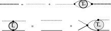
Figure 2: Upper part: The Dyson equation for the physical pion (thick dashed lines) for which the mass operator has been extracted from the scattering of the quasibosons in an RPA equation. Lower part: The scattering equation for a pair of quasi-sigma (thin full lines) and quasi-pion (thin dashed lines).

This can in fact be done analytically and yields

$$\Omega^{2}_{\nu}\,=\,{\cal E}^{2}_{\pi}(0)\quad+\quad\frac{4\lambda_{0}^{4}s^{2}\Sigma_{\pi\sigma}(\Omega^{2}_{\nu})}{1\,\,-\,\,2\lambda_{0}^{2}\Sigma_{\pi\sigma}(\Omega^{2}_{\nu})}$$ (25)

where $\Sigma_{\pi\sigma}$ is the contribution of the (quasi) pion-sigma bubble to the pion selfenergy given by

$$\Sigma_{\pi\sigma}(\Omega^{2}_{\nu})\,=\,\int\frac{d^{3}\vec{q}}{(2\pi)^{3}}\quad\frac{{\cal E}_{\pi}(q)+{\cal E}_{\sigma}(q)}{2{\cal E}_{\pi}(q){\cal E}_{\sigma}(q)}\frac{1}{\Omega^{2}_{\nu}\,-\,({\cal E}_{\pi}(q)+{\cal E}_{\sigma}(q))^{2}}.$$ (26)

Using the identity

$$\Sigma_{\pi\sigma}(0)\,=\,\frac{I_{0}\,\,-\,\,J_{0}}{{\cal E}^{2}_{\pi}(0)-{\cal E}^{2}_{\sigma}(0)},$$ (27)

we obtain after some algebra,

$$\Omega^{2}_{\nu}\,=\,\frac{2\lambda_{0}^{2}\left[{\cal E}_{\pi}^{2}(0)\,-\,{\cal E}_{\sigma}^{2}(0)\right]\left[\Sigma_{\pi\sigma}(0)\,-\,\Sigma_{\pi\sigma}(\Omega^{2}_{\nu})\right]}{1\quad-\quad 2\lambda_{0}^{2}\Sigma_{\pi\sigma}(\Omega^{2}_{\nu})}\quad+\quad\frac{c}{s}\ .$$ (28)

In the chiral limit $(c=0)$ the zero-energy solution is now manifest (independent of any regularization scheme).
It is interesting to ask: What is the Goldstone boson dispersion relation? i.e. what is the behavior of the spurious mode under spatial translations. For this purpose we shall use as the generator of the spurious mode the time component of the axial vector current $A^{a\,0}_{5}(x)$ rather than the axial charge. The Fourier transform of the latter allows to pick up the spurious mode at any finite three momentum. To show that $A^{a\,0}_{5}(x)$ can generate a spurious mode we recall the PCAC relation

$$\partial_{\mu}A_{5}^{a\,\mu}({\bf x})=c\pi^{a}({\bf x}).$$ (29)

Using Heisenberg’s equation of motion, after Fourier transformation, this can be simply expressed as

$$\left[H,A_{5}^{a\,0}({\vec{p}})\right]\,\,+\,\,{\vec{p}}{\vec{A}}_{5}^{a}({\vec{p}})\,\,=\,\,-ic\pi^{a}({\vec{p}})$$ (30)

In the chiral limit the single-pion part of the RPA operator then generates a solution of finite three-momentum which has the following property

$$\langle{RPA}|\left[\delta Q_{\nu}\,\,,\,\,\left[H,A_{5}^{a\,0}({\vec{p}})\right]\right]|{RPA}\rangle\,\,+\,\,{\vec{p}}\langle{RPA}|\left[\delta Q_{\nu}\,,\,{\vec{A}}_{5}^{a}({\vec{p}})\right]|{RPA}\rangle\,\,=\,\,0.$$ (31)

This clearly indicates that for pions at rest $({\vec{p}}={\vec{0}})$ again a zero-frequency solution exist. To make the dispersion relation explicit we consider the following excitation operator

$$Q_{\nu}^{+}({\vec{p}})=X^{1}_{\nu}({\vec{p}})\alpha^{a\,+}_{-\vec{p}}\,\,-\,\,Y^{1}_{\nu}({\vec{p}})\alpha^{a}_{\vec{p}}\quad+\quad\sum_{q}\left[X_{\nu}^{2}({\vec{p}},{\vec{q}})\beta^{+}_{{\vec{q}}-{\vec{p}}}\alpha^{a\,+}_{-{\vec{q}}}\,\,-\,\,Y_{\nu}^{2}({\vec{p}},{\vec{q}})\beta_{{\vec{p}}-{\vec{q}}}\alpha^{a}_{\vec{q}}\right]$$ (32)

which is the extension of eq. (23) to finite three-momenta. After some algebra the RPA frequencies can be expressed as

$$\Omega^{2}_{\nu}(\vec{p})\,=\,\frac{2\lambda^{2}\left[{\cal E}_{\pi}^{2}(0)\,-\,{\cal E}_{\sigma}^{2}(0)\right]\left[\Sigma_{\pi\sigma}(0)\,-\,\Sigma_{\pi\sigma}(\Omega^{2}_{\nu},{\vec{p}})\right]}{1\quad-\quad 2\lambda^{2}\Sigma_{\pi\sigma}(\Omega^{2}_{\nu},{\vec{p}})}\quad+\quad\frac{c}{s}\quad+\quad{\vec{p}}^{2}$$ (33)

with

$$\Sigma_{\pi\sigma}(\Omega^{2}_{\nu},{\vec{p}})\,=\,\int\frac{d^{3}\vec{q}}{(2\pi)^{3}}\quad\frac{{\cal E}_{\pi}({\vec{q}})+{\cal E}_{\sigma}({\vec{p}}-{\vec{q}})}{2{\cal E}_{\pi}({\vec{q}}){\cal E}_{\sigma}({\vec{p}}-{\vec{q}})}\frac{1}{\Omega^{2}_{\nu}\,-\,({\cal E}_{\pi}({\vec{q}})+{\cal E}_{\sigma}({\vec{p}}-{\vec{q}}))^{2}}.$$ (34)

Using the fact that the $\pi\sigma$ selfenergy is Lorentz invariant one easily verifies that

$$\Omega^{2}_{\nu}(\vec{p})\,=\,\Omega^{2}_{\nu}(0)\quad+\quad{\vec{p}}^{2}$$ (35)

as it should be. Note that this result remains valid away from the chiral limit.

4 Finite Temperature HFB-RPA

In a first step towards a nonperturbative description of the chiral phase transition we now extend the formalism to finite temperature by using well-known methods available in the literature[8, 9, 10]. As we have demonstrated in the previous sections, the HFB-RPA has proven successful in preserving the symmetry which is manifest through the presence of the spurious mode in the single pion RPA spectrum. The same is to be expected at finite temperature. Let us now first come to the mean field problem. We recall therefore that the thermodynamics of a gas of pions and sigmas at given temperature $T$ is governed by the free energy $\Omega$

$$\Omega=\langle{H}\rangle-TS.$$ (36)

where $\langle{H}\rangle$ is the thermal expectation value of the Hamiltonian in eq. (9) and $S$ denotes the entropy. In thermal equilibrium the distribution of maximum entropy is the one which minimizes $\Omega$. The entropy then reads

$$S=k_{B}\sum_{\nu}\left[(1+f_{\nu})ln(1+f_{\nu})-f_{\nu}lnf_{\nu}\right]$$ (37)

where $k_{B}$ is the Boltzmann constant and $f_{\nu}$ is the usual bosonic distribution functions. The sum $\nu$ includes the number of species as well as the three momentum q.

In analogy to the zero-temperature case we can perform a temperature-dependent Bogoliubov rotation for both the $\pi$ and $\sigma$ fields. By making use of the Bloch-De Dominicis theorem [11] normal ordering on the rotated creation and annihilation operators can be carried out and one straightforwardly arrives at the HFB expression for the free energy

$$\Omega \,=\, {\cal H}_{0}(v_{T},y_{T},s_{T})-TS,$$

$${\cal H}_{0}(v_{T},y_{T},s_{T}) \,=\, \sum_{q}\,\omega_{q}(3v^{2}_{T,q}+y^{2}_{T,q}+2)\,+\,\frac{3\lambda_{0}^{2}}{4}\left[J^{2}_{T}+5I^{2}_{T}+2I_{T}J_{T}\right]$$ (38)

$$\,+\, \frac{3\lambda_{0}^{2}s_{T}^{2}}{2}\left[I_{T}+J_{T}\right]\,+\,\frac{\mu_{0}^{2}s_{T}^{2}}{2}+\frac{\lambda_{0}^{2}s_{T}^{4}}{4}-cs_{T}$$

where ${\cal H}_{0}(v_{T},y_{T},s_{T})$ is just the expectation value of H on the grand canonical ensemble. Minimizing $\Omega$ with respect to $u_{T,q}$ and $x_{T,q}$ and $s_{T}$ while keeping the canonical normalization of the Bogoliubov factors as in eq. (6) then leads to the following identities

$$\eta^{T} = \frac{x_{T,0}+y_{T,0}}{\sqrt{\mu}}\left[3\lambda_{0}^{2}s_{T}I_{T}+3\lambda_{0}^{2}s_{T}J_{T}+\lambda_{0}^{2}s_{T}^{3}+\mu_{0}^{2}s_{T}-c\right]\,=\,0$$

$$c^{T}_{\pi}(q) = \omega_{q}(u_{T,q}v_{T,q})+\frac{\lambda_{0}^{2}}{2}\frac{(u_{T,q}+v_{T,q})^{2}}{2\omega_{q}}\left[5I_{T}+J_{T}+s_{T}^{2}\right]\,\,=\,\,0$$

$$c^{T}_{\sigma}(q) = \omega_{q}(x_{T,q}y_{T,q})+\frac{3\lambda_{0}^{2}}{2}\frac{(x_{T,q}+y_{T,q})^{2}}{2\omega_{q}}\left[I_{T}+J_{T}+s_{T}^{2}\right]\,\,=\,\,0$$

$${\cal E}^{T}_{\pi}(q) = \omega_{q}(u_{T,q}^{2}+v_{T,q}^{2})+\lambda_{0}^{2}\frac{(u_{T,q}+v_{T,q})^{2}}{2\omega_{q}}\left[5I_{T}+J_{T}+s_{T}^{2}\right]$$

$${\cal E}^{T}_{\sigma}(q) = \omega_{q}(x_{T,q}^{2}+y_{T,q}^{2})+3\lambda_{0}^{2}\frac{(x_{T,q}+y_{T,q})^{2}}{2\omega_{q}}\left[I_{T}+J_{T}+s_{T}^{2}\right]$$ (39)

where the definitions are as in the zero-temperature case and ${\cal H}_{0}$ takes the same form as in eq. (10). The loop integrals $I_{T}$ and $J_{T}$ are now given by

$$I_{T}=\int\frac{d^{3}\vec{q}}{(2\pi)^{3}}\quad\frac{1+2f_{\pi}(q)}{2\omega_{q}(u_{T,q}-v_{T,q})^{2}},\quad\quad\quad J_{T}=\int\frac{d^{3}\vec{q}}{(2\pi)^{3}}\quad\frac{1+2f_{\sigma}(q)}{2\omega_{q}(x_{T,q}-y_{T,q})^{2}}$$ (40)

and the quasi-particle masses ${\cal E}^{T}_{\pi}$, ${\cal E}^{T}_{\sigma}$ and the condensate $s_{T}$ take the form

$${\cal E}_{\pi}^{T}(0)^{2} = \mu_{0}^{2}+\lambda_{0}^{2}\left[5I_{T}+J_{T}+s_{T}^{2}\right]$$

$${\cal E}_{\sigma}^{T}(0)^{2} = \mu_{0}^{2}+3\lambda_{0}^{2}\left[I_{T}+J_{T}+s_{T}^{2}\right]$$

$$c = s_{T}\left[\mu_{0}^{2}+\lambda_{0}^{2}s_{T}^{2}+3\lambda_{0}^{2}\left(I_{T}+J_{T}\right)\right]$$ (41)

which is of identical form as the $T=0$ expressions.

We now move on to the RPA problem at finite $T$. In the spirit of the zero-temperature RPA an operator $Q_{\nu}^{+}$ is used which contains the same excitations as the symmetry generator. Therefore $Q_{\nu}^{+}$ is given by

$$Q_{\nu}^{+}=X^{1}_{\nu}\alpha^{a\,+}_{0}\,\,-\,\,Y^{1}_{\nu}\alpha^{a}_{0}\,\,+\,\,\sum_{q}\left[X_{\nu}^{2}(q)\beta^{+}_{q}\alpha^{a\,+}_{-q}\,\,-\,\,Y_{\nu}^{2}(q)\beta_{-q}\alpha^{a}_{q}\,\,+\,\,X_{\nu}^{3}(q)\beta_{-q}\alpha^{a\,+}_{-q}\,\,-\,\,Y_{\nu}^{3}(q)\beta^{+}_{q}\alpha^{a}_{q}\right]$$ (42)

which now contains additional terms of ’mixed’ type. The analogous equations of motion have been worked out in refs. [9, 10] and read

$$\langle{\left[\delta Q_{\nu}\,\,,\,\,\left[H\,,\,Q_{\nu}^{+}\right]\right]}\rangle=\Omega_{\nu}\langle{\left[\delta Q_{\nu}\,,\,Q_{\nu}^{+}\right]}\rangle$$ (43)

where the average is to be taken in the grand ensemble. The RPA operator (42) now generates a set of six equations for the various amplitudes which can be written as

$$\int d^{3}{\vec{p}}{\cal M}_{ij}(q,p){\chi}_{j}(p)=\Omega^{T}_{\nu}{\cal N}_{ij}(q){\chi}_{j}(q)$$ (44)

where ${\cal M}(q,p)$ is the $6\times 6$ RPA matrix to be inverted, $\Omega^{T}_{\nu}$ and $\chi(p)$ are the eigenvalues and 6-column eigenvectors respectively, and finally ${\cal N}(q)$ is the diagonal matrix norm :

$${\cal N}_{11}(q) = -{\cal N}_{22}(q)=1$$

$${\cal N}_{33}(q) = -{\cal N}_{44}(q)=1+f_{\pi}(q)+f_{\sigma}(q)$$

$${\cal N}_{55}(q) = -{\cal N}_{66}(q)=f_{\sigma}(q)-f_{\pi}(q)$$

The normalization condition for the eigenvectors is

$$<\left[Q_{\nu},Q^{+}_{\nu^{\prime}}\right]> \,=\, \left(\mid X^{1}_{\nu}\mid^{2}-\mid Y^{1}_{\nu}\mid^{2}\right)\,+\,\sum_{q}\left[\left[1+f_{\pi}(q)+f_{\sigma}(q)\right]\left(\mid X^{2}_{\nu}(q)\mid^{2}-\mid Y^{2}_{\nu}(q)\mid^{2}\right)\right.$$ (46)

$$\,+\, \left.\left[f_{\sigma}(q)-f_{\pi}(q)\right]\left(\mid X^{3}_{\nu}(q)\mid^{2}-\mid Y^{3}_{\nu}(q)\mid^{2}\right)\right]\,=\,\delta_{\nu\nu^{\prime}}$$

The solution of the eigenvalue problem in eq.(44) gives

$$\Omega_{\nu}^{2}\,=\,{\cal E}^{T\,2}_{\pi}(0)\quad+\quad\frac{4\lambda_{0}^{4}s_{T}^{2}\Sigma^{T}_{\pi\sigma}(\Omega^{2}_{\nu})}{1-2\lambda_{0}^{2}\Sigma_{\pi\sigma}^{T}(\Omega_{\nu}^{2})}$$ (47)

where

$$\Sigma_{\pi\sigma}^{T}(\Omega_{\nu}^{2})\,=\,\int\frac{d^{3}{\vec{p}}}{(2\pi)^{3}}\left[\frac{{\cal E}^{T}_{\pi}(p)+{\cal E}^{T}_{\sigma}(p)}{2{\cal E}^{T}_{\pi}(p){\cal E}^{T}_{\sigma}(p)}\frac{1+f_{\pi}(p)+f_{\sigma}(p)}{\Omega_{\nu}^{2}-({\cal E}^{T}_{\pi}(p)+{\cal E}^{T}_{\sigma}(p))^{2}}\,+\,\frac{{\cal E}^{T}_{\pi}(p)-{\cal E}^{T}_{\sigma}(p)}{2{\cal E}^{T}_{\pi}(p){\cal E}^{T}_{\sigma}(p)}\frac{f_{\sigma}(p)-f_{\pi}(p)}{\Omega_{\nu}^{2}-({\cal E}^{T}_{\pi}(p)-{\cal E}^{T}_{\sigma}(p))^{2}}\right]$$ (48)

and the Bose occupation factors are given by

$$f_{\pi,\sigma}(p)=\left[exp(\frac{{\cal E}_{\pi,\sigma}^{T}(p)}{T})-1\right]^{-1}$$ (49)

One verifies that in the zero-temperature limit the previous HFB-RPA results are recovered.
For the physical interpretation of these results we first address the question whether the FTHFB-RPA is able to describe the two realizations of the symmetry i.e. the Wigner phase and the Goldstone phase. In the Goldstone phase the vacuum condensate $s_{T}$ is finite and the bare mass $\mu_{0}^{2}$ negative such that the third equation in (41) is satisfied in the chiral limit ($c=0$). There exists therefore a Goldstone mode in the theory and the symmetry is no longer manifest in the particle spectrum which means that the masses of the $\sigma$ and the $\pi$ are different. In the zero-temperature case we have demonstrated that HFB-RPA scheme is consistent with these requirements.

There is, however, an alternative solution of the third equation in (41). Suppose the condensate $s_{T}$ vanishes at some temperature. In this case the three-particle coupling disappears from the interaction Hamiltonian, as can be seen explicitly from eq. (9). The single-particle state no longer couples to two-particle states and the only contribution of the single-particle masses is the one that comes from the four-point interactions in the mean-field calculation. This can also be checked explicitly from the RPA eigenvalues. It is now easy to see from eqs. (41) that the masses become degenerate i.e. ${\cal E}_{\pi}={\cal E}_{\sigma}$ and we are in the Wigner mode. The question is whether this is inconsistent with the fact that $Q^{a}_{5}$, the generator of the symmetry, commutes with the Hamiltonian which leads to a spurious solution of the RPA in the Goldstone phase. First one should note that if the masses are equal then the thermal occupation factors for both the pion and the sigma are the same. This leads to ${\cal N}_{55}(q)={\cal N}_{66}(q)=0$ implying that the RPA spurious mode cannot be normalized. Secondly, from equation (47) we see that to have the zero frequency mode, one must fulfill the following condition

$$0\,=\,{\cal E}^{T\,2}_{\pi}(0)\,+\,\frac{4\lambda_{0}^{4}s_{T}^{2}\Sigma^{T}_{\pi\sigma}(0)}{1-2\lambda_{0}^{2}\Sigma_{\pi\sigma}^{T}(0)}$$ (50)

In analogy to eq. (27) one can prove the following identity

$$\Sigma^{T}_{\pi\sigma}(0)\,=\,\frac{I_{T}\,\,-\,\,J_{T}}{{\cal E}^{T\,2}_{\pi}(0)-{\cal E}^{T\,2}_{\sigma}(0)},$$ (51)

which is only true, however, if all six terms in the excitation operator $Q^{+}_{\nu}$ (eq. (42) are kept. Now the condition for a spurious mode solution can be simply recast as

$$\frac{c}{s_{T}}\,=\,0$$ (52)

which means that the ratio of the symmetry breaking term in the Lagrangian and the condensate must vanish to allow a zero-energy solution. This can only happen for finite $s_{T}$ i.e. in the Goldstone phase. Once the Wigner phase is reached this condition can no longer be satisfied. This reiterates the fact that the spurious mode is a manifestation of a broken symmetry which disappears once the latter is restored.

5 Conclusions and outlook

In summary we have presented a non-perturbative method based on the well-known selfconsistent QRPA formalism for studying the linear $\sigma$-model in the bosonic sector. Being ’symmetry conserving’ the method yields a zero mode in the chiral limit. This is required by Goldstone’s theorem for a spontaneously broken symmetry. While, at field level, the pion acquires a mass through the BCS mechanism irrespective of the explicit symmetry breaking term in the Lagrangian the inclusion of RPA correlations removes this artifact. We have also demonstrated that the extension of the QRPA to finite temperature is workable and reproduces the expected result that the zero mode persists at finite temperature. Applications to the $SU(3)$-case as well as the inclusion of fermions are straightforward and are being considered. This will hopefully provide new insight into the nature of the chiral phase transition. Since, in contrast to Nambu-Jona-Lasinio type models, the linear $\sigma$-model is renormalizable a program of non-perturbative renormalisation should be persued in order to assess its impact on the physics. Despite the selfconsistency of the mean-field equations a solution of this problem does not seem out of reach. A challenging problem is the application of the formalism to the two-pion case. Here one attempts to build a scattering equation which is consistent with the low-energy theorems required by the symmetry. As is known from the analogous fermionic problem higher RPA schemes have to be employed. In particular the second RPA [12, 13] is also ’symmerty conserving’. Its bosonic analog is easy to construct but some conceptual problems remain to be resolved.

References

• [1] J. Gasser and H. Leutwyler, Ann. Phys. (N.Y.) 158 (1984) 142.
• [2] Z. Aouissat, R. Rapp, G. Chanfray, P. Schuck, J. Wambach, Nucl. Phys. A581 (1995) 471.
• [3] E. R. Marshalek Nucl. Phys. A224 (1974) 221.
• [4] M. Gell-Mann and M. Levy, Nuovo Cim.16, 53 (1960).
• [5] B. W. Lee, Nucl. Phys. B9 (1969)649.
• [6] D. J. Rowe, Rev. Mod. Phys. 40 (1968)
• [7] P. Ring, P. Schuck, The Nuclear Many-Body Problem, (Springer-Verlag, 1980).
• [8] A. L. Goodman, Nucl. Phys. A352 (1981) 30.
• [9] H. M. Sommermann, Ann. Phys. 151 (1983) 163.
• [10] K. Tanabe and K. Sugawara-Tanabe, Prog. Theo. Phys. Vol 76, n2 (1986) 356.
• [11] C. Bloch, C. De Dominicis, Nucl. Phys. 7, (1956) 459; 10, (1959) 181, 509.
• [12] S. Drożdż, S. Nishizaki, J. Speth, J. Wambach, Phys. Rep. 197 (1990) 1.
• [13] C. Yannouleas, M. Dworzecka, J.J. Griffin, Nucl. Phys. A397 (1983) 239.