A Quantum-Mechanical Equivalent-Photon Spectrum for Heavy-Ion Physics

Abstract

In a previous paper, we calculated the fully quantum-mechanical cross section for electromagnetic excitation during peripheral heavy-ion collisions. Here, we examine the sensitivity of that cross section to the detailed structure of the projectile and target nuclei. At the transition energies relevant to nuclear physics, we find the cross section to be weakly dependent on the projectile charge radius, and to be sensitive to only the leading momentum-transfer dependence of the target transition form factors. We exploit these facts to derive a quantum-mechanical “equivalent-photon spectrum” valid in the long-wavelength limit. This improved spectrum includes the effects of projectile size, the finite longitudinal momentum transfer required by kinematics, and the response of the target nucleus to the off-shell photon.

1 Introduction

In the previous decade, relativistic heavy-ion beams have become a useful tool for the study of electromagnetic processes in nuclei. Applications have included studies of nuclear astrophysics[1], nuclei far from stability[2], and searches for multi-phonon excitations in nuclei[3]. In these experiments, cross sections that are difficult to measure by other means are amplified by the projectile charge, and, in the case of relativistic projectiles, by the contraction of the projectile’s electric field into a sharp pulse.

Almost exclusively, the data from these experiments have been analyzed using the semi-classical Weizsäcker-Williams method of virtual quanta[4], in which the cross section for the heavy-ion-induced reaction is calculated by integrating the cross section for the analogous real-photon process over a flux of photons that is “equivalent” to those that make up the electric field of the projectile. In its simplest form, the pulse of equivalent photons is obtained from the boosted Coulomb field of the projectile by equating the classical Poynting flux onto the target to the energy flux carried by the pulse of equivalent photons. The semi-classical spectrum has been generalized to include arbitrary multipoles[5], projectile structure[6] and Coulomb scattering effects[7]. Attempts to move beyond the semi-classical picture of these processes have been thwarted by lack of information about the structure of the target nucleus[8]. Furthermore, there has been little motivation for improvement because the semi-classical spectrum, when used in conjunction with data from real-photon processes, provides model-independent results for cross sections measured in heavy-ion collisions[9].

Recently, we have undertaken a program to systematically examine corrections to the semi-classical picture[10] [11], and have found significant deviations from the predictions of the Weizsäcker-Williams method for the mildly relativistic collisions ($\gamma<2-3$) that constitute a significant fraction of the available data. The aim of the present work is to expand on the results of reference 10, examining the sensitivity of the cross section to nuclear structure inputs. Having determined which inputs are essential to extracting the correct physical cross sections, we construct a simple model that incorporates these features, and is valid in the limit of low transition energies. This allows us to obtain a new, fully quantum-mechanical expression for an “equivalent-photon spectrum” that can be used with measured photoabsorption cross sections in exactly the same fashion as the semi-classical expression.

The paper is structured as follows: In the next section, we briefly review the results of reference 10, emphasizing the interplay between the different length scales that determine the cross sections measured in heavy-ion collisions. The third section is devoted to a comparison of the exact numerical results for the cross sections using an assortment of parametrizations for the projectile form factors and target transition densities. In the fourth section, we use the results from these comparisons to construct a simple model for the form factors and transition densities that incorporates the important physical parameters of the projectile and target. This allows us to extract a new effective photon spectrum that may be used in the same fashion as the Weizsäcker-Williams spectrum. In the last section, we compare the predictions obtained using the new spectrum with selected data from heavy-ion collisions.

2 Quantum Cross Section for Electromagnetic Processes Induced By Heavy Ions

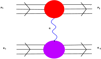
Figure 1: Feynman diagram for electromagnetic excitation in a peripheral heavy-ion collision.

We begin with a review of the results of Ref. [10], where the cross section for nuclear excitation induced by the electromagnetic fields of a passing heavy ion was derived in the first Born approximation. The relevant Feynman diagram is shown in Fig. 1. A virtual photon of momentum $q^{\mu}$ is exchanged between the target and projectile nuclei, producing an excitation in the target of energy $\omega_{T}$. (As a matter of convention, the nucleus that gets excited is considered to be the target.) The cross section for simultaneously exciting both nuclei has been shown to be small[11] at this level of approximation in the fine structure constant. The lack of projectile excitation and the large masses of the nuclei combine to determine both the energy transfer and the component of the momentum transfer along the direction of the projectile momentum. These are given, in the target rest frame, by

$$q_{0} = \omega_{T}$$

$${\bf q}^{\parallel} = \omega_{T}/\beta,$$ (1)

where $\beta$ is the projectile velocity. Our metric is such that $q^{2}\equiv q^{2}_{0}-{\bf q}^{2}$ .

In Ref. [10], the cross section was written in the compact form

$$\sigma_{HI} = {2(Z_{P}\alpha)^{2}\over\beta^{2}}\int\,d\omega_{T}\,\rho(\omega_{T})\int_{\omega_{T}/\beta}^{\sqrt{(\omega_{T}/\beta)^{2}+{\bf q}_{max}^{2}}}|{\bf q}|d|{\bf q|}|F_{P}(q^{2})|^{2}\left[{1\over\gamma^{2}}{|F^{T}({\bf q})|^{2}\over(\omega_{T}^{2}-{\bf q}^{2}){\bf q}^{2}}\right.$$ (2)

$$\left.\qquad\qquad\qquad\qquad\qquad\qquad-{|F^{T}({\bf q})|^{2}\over(\omega_{T}^{2}-{\bf q}^{2})^{2}}+{2|F^{C}({\bf q})|^{2}\over{\bf q}^{4}}\right],$$

where $Z_{P}$ is the projectile’s charge, $F_{P}(q^{2})$ is the elastic form factor of the projectile, $F^{T}({\bf q})$ and $F^{C}({\bf q})$ are the transverse and Coulomb form factors of the target, $q_{max}$ is a phenomenological cutoff on the transverse momentum transfer required to account for strong absorption effects, $\rho(\omega_{T})$ is the density of states in the target with excitation energy $\omega_{T}$, and $\gamma=(1-\beta^{2})^{-1/2}$.

From this expression, it is easy to see how the semi-classical limit is realized. As $\gamma$ becomes large, the lower limit of the ${\bf q}$ integration approaches $\omega_{T}$. When this happens, the behavior of the integral is dominated by the rapid variation of the poles at $q^{2}=0$ in the photon propagators. The nuclear densities and form factors vary much more slowly with $q^{2}$, and are effectively frozen at their values for $q^{2}=0$. The third term in Eq. 2, which has no pole at $q^{2}=0$, is small compared to the first two, which grow logarithmically with $\gamma$. Thus, the cross section factorizes neatly into a product of the same matrix elements that appear in the excitation cross section for real photons, times an “equivalent photon number”. The latter is a function only of the $\omega_{T}$, $q_{max}$, and $\gamma$.

Outside of the large-$\gamma$ limit, there is no simple factorization of the quantum cross section, Eq. (2), so that there is no possibility for reconciliation with the semi-classical expression without further approximations. The differences between the semi-classical approximation and the full result are even more striking when the transverse momentum cutoff, $q_{max}$, is removed to $\infty$. In this limit, the semi-classical cross section diverges logarithmically, while the full expression for the cross section remains finite. There are three additional regulating factors in the full cross section, which tend to lower the cross section even when $q_{max}$ is finite. The first factor arises because of the finite size of the projectile. The magnitude of the three-momentum transfer in the projectile’s rest frame is given by $\sqrt{-q^{2}}\geq\omega_{T}/\gamma\beta$, and the degree to which the protons in the projectile act coherently on the target is reduced at large $q$. This produces a cutoff governed by the size of projectile, $R_{P}$. The falloff of the target’s excited state wave function at high momentum produces a corresponding second regulator governed by the target size, $R_{T}$. In the absence of both these effects, the cross section would still remain finite as a result of the ${\bf q}^{-4}$ dependence of the integrals appearing in Eq. 2. This third factor effectively cuts off the integrals at momentum scales of the order of $\omega_{T}$. If, in order to agree with semi-classical estimates, one chooses $q_{max}\approx{1\over(R_{T}+R_{P})}$, the situation becomes complicated, as all the cutoffs are of comparable size. Without further study, it impossible to determine which of these factors are most important in relation to the measured cross section.

3 Effects of Nuclear Structure

In this section, we examine the effects of the detailed form factors (or transition densities) on the cross sections calculated with Eq. 2. These effects are naturally divided into projectile and target structure, and we begin with the former.

3.1 Projectile Structure

In the semi-classical description, the projectile is assumed to be a point charge, and only the long-range Coulomb field of the projectile generates the photon flux. From Eq. 2, it is apparent that the extended nature of the projectile enters the cross section through its elastic form factor, $F_{P}(q^{2})$, which accounts for the incoherence of the electromagnetic fields produced by spatially separate regions of the projectile. The size of this effect, which tends to decrease the heavy-ion cross section, is governed by $(\omega_{T}R_{P}/\beta\gamma)^{2}$, where $R_{P}$ is the charge radius of the projectile. For light-target, heavy-projectile combinations, there is no guarantee that this is small unless $\gamma$ is large.

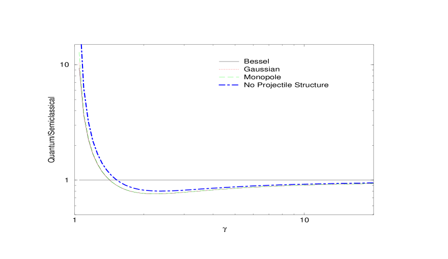
Figure 2: The dependence of the Coulomb-excitation cross section on the finite size of the projectile. The figure shows the ratio of the full quantum result to the standard semi-classical approximation for the cross section for a 20 MeV dipole excitation of ⁴¹Ca by a ¹⁹⁷Au ion. Results are shown for a point projectile (dot-dash curve) and for three different forms for $F_{P}(q^{2})$ with the same charge radius. For low-projectile energies the predictions of the usual semi-classical approximation deviate significantly from the full quantum results even for point-like projectiles. When the finite size of the projectile is included, the cross sections shows sensitivity to the charge radius of the projectile, but not to the detailed form of the projectile charge distribution. For low-energy projectiles ($\approx$ 50 MeV/nucleon) the cross section is reduced by a factor of 2-3 relative to the point-projectile result. At $\gamma$=2 the calculated cross section is reduced by $7\%$ relative to the point-projectile results, and the relative reduction decreases as the projectile energy increases.

In Fig. 2, we demonstrate the effect of the finite size of the projectile on the calculated cross section. The ratio of the quantum to classical cross sections for a 20 MeV dipole excitation of a mass 41 target by a ¹⁹⁷Au projectile, as a function of projectile energy is shown. Here, and in all the calculations to follow, we choose $q_{max}=1/b_{min}$, where

$$b_{min}=(1.34\,{\rm fm})\left(A_{P}^{1/3}+A_{T}^{1/3}-0.75\cdot(A_{P}^{-1/3}+A_{T}^{-1/3})\right)$$ (3)

is a commonly used minimum-impact-parameter cutoff in semi-classical calculations[3][12]. The four curves represent the results of assuming either a point projectile(dot-dash curve), or a projectile with mean-square charge radius of $\langle r^{2}\rangle_{ch}^{1/2}=$ 5.4 fm and form factor parametrized by

$$F_{P}(q^{2}) = {3j_{1}(x)\over x}\hskip 158.99377pt\mbox{ (Bessel)}$$ (4)

$$= \exp(-x^{2})\hskip 133.69994pt\mbox{(Gaussian)}$$

$$= {1\over 1+x^{2}}\hskip 144.54pt\mbox{(Monopole)}\>,$$

with $x=\sqrt{-q^{2}r^{2}/6}$, and $r$ the root-mean-square charge radius of the projectile. For each curve we have assumed that target transition densities are given by the Goldhaber-Teller model[13].

For low-energy projectiles ($\approx$ 50 MeV/nucleon), the calculated cross section is sensitive to the finite size of the projectile, and is smaller by a factor of 2-3 than the point-projectile result. For relativistic projectiles, the reduction in cross section is less dramatic, being about 7% at $\gamma=2$ and decreasing as the projectile energy increases. Once the charge radius is fixed, however, the resulting cross section is insensitive to the further details of the form factor, except at the lowest projectile energies, where a variation $\approx$ 20% remains. We conclude that the effect of projectile size is non-negligible for many nuclear transitions, particularly when the projectile energy is low. We note, however, that the effect is smaller for lower-energy transitions, since the minimum $q^{2}$ of the virtual photon varies as $\omega_{T}^{2}$.

3.2 Target Structure Effects

We now turn to the issue of target structure. In the classical prescription, the target is assumed to respond to the electromagnetic field of the passing projectile in exactly the same fashion as it would to a real photon. Hence, for the majority of the transitions of interest, the long-wavelength approximation should be valid. In the quantum case, this is not guaranteed, since the momentum transfer is bounded from below by $\omega_{T}/\beta>\omega_{T}$, so that higher moments of the transition density may play a larger role than they do for processes mediated by real photons. To calculate the quantum cross sections we used transition form factors taken from two models. The first of these represents a generalized collective model for nuclear giant resonances[13], which is motivated by the Goldhaber-Teller (GT) model for the giant dipole resonance. The second set of transitions are the shell-model form factors classified[14] by their SU(3) symmetries.

In the generalized GT model, the transition densities are taken to be the gradient of a spherically symmetric ground-state density. These collective transition densities are then correct to leading order in the long-wavelength limit, and the form factors for a given multipole $\ell$ are given by

$$|F^{C}_{\ell}({\bf|q|})|^{2} = \ell\,C_{\ell}\,j_{\ell}^{2}({|\bf q|}R_{T})\,,$$

$$|F^{T}_{\ell}({\bf|q|})|^{2} = {(\ell+1)\over\ell}{\omega_{T}^{2}\over\bf q^{2}}|F_{\ell}^{C}({\bf|q|})|^{2}\;\;\;.$$ (5)

Here $R_{T}$ is the target charge radius, and $C_{\ell}$ is a constant chosen so as to saturate the appropriate photonuclear sum rule for multipole $\ell$[10].

In the shell model, appropriate linear combinations of the single-particle transitions can provide descriptions of either giant resonance states or non-collective states. By examining each of these we can explore the sensitivity of the cross section to a wide range of transitions, including the so called “retarded” transitions. (The retarded transitions are those that do not contribute to the real-photon cross section in the leading order of the long-wavelength approximation.) The separation into unretarded and retarded transitions can be achieved by classifying the shell-model form factors by their transformation properties under the SU(3) symmetry[14, 15, 16] of the three dimensional harmonic oscillator. This classification scheme has the advantage of allowing us to identify easily those form factors that dominate the cross section in the long-wavelength limit.

Table I lists the expressions for the dipole Coulomb and transverse electric form factors classified under SU(3). As discussed in the appendix, these are linear combinations of the usual $jj$-coupled transitions. Following Donnelly and Haxton[17], the form factors are expressed in terms of a polynomial in $y$, where $y\equiv(b{\bf q}/2)^{2}$ and $b$ is the shell-model oscillator size parameter. For a dipole transition between oscillator orbits with $Q_{1}$ and $Q_{2}$ quanta there are $(Q_{1}+Q_{2}+1)/2$ distinct form factors, and these are labelled with SU(3) quantum numbers ($\lambda,\mu)=(1,0),\cdots(Q_{1}-1,Q_{2}-1),(Q_{1},Q_{2})$. The maximum power of $y$ appearing in any form factor is determined only by the orbitals involved in the transitions and is equal to $(Q_{1}+Q_{2})/2$. The lowest power of $y$ is determined by $(\lambda,\mu)$ and is equal to $(\lambda+\mu)$/2. Thus, the SU(3) scheme provides the required linear combinations of the shell-model form factors, separating them into an unretarded transition and a set of transitions retarded to various orders in ${\bf q}^{2}$. In the long-wavelength approximation, only the $(\lambda,\mu)=(1,0)$ form factor contributes in leading order, and it contains all the allowed B(E1) strength. The (1,0) form factor is the shell-model equivalent of the Goldhaber-Teller giant resonance, and can be obtained by differentiating the ground-state density distribution. The $(\lambda,\mu)=(2,1)$ and higher SU(3) form factors represent the retarded dipole transitions, and do not contribute to real photon processes in the long-wavelength limit.

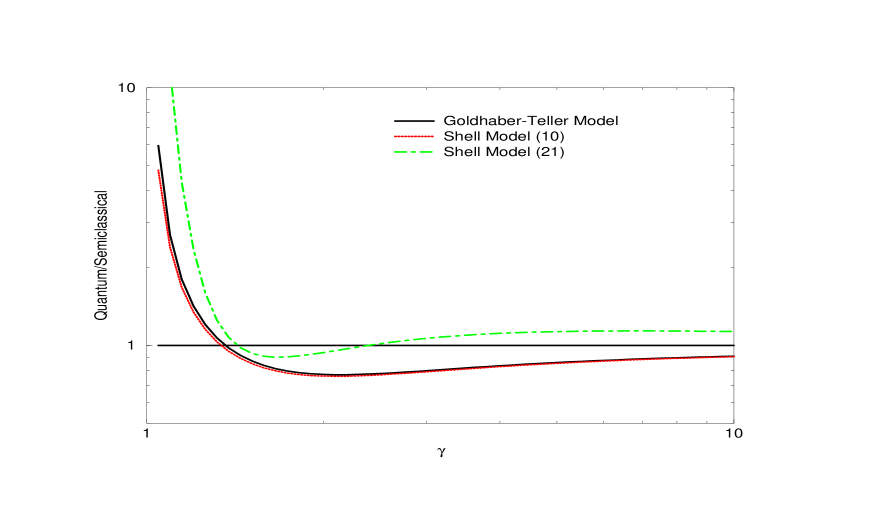
Figure 3: Ratio of the full quantum result to the standard semi-classical approximation for the cross section of a 20 MeV dipole excitation in ¹⁷O by a ¹⁹⁷Au ion. The transition form factors for ¹⁷O are described by either the Goldhaber-Teller Model, or by shell-model densities transforming as $(1,0)$ or $(2,1)$ representations of SU(3). The Goldhaber-Teller and the ($\lambda,\mu$)=(1,0) transition form factors have the same leading-order dependence in $\mid$q$\mid$ and their calculated cross sections are very similar. The (2,1) transition form factor does not contribute in leading order in the long-wavelength approximation, and shows a markedly different cross-section ratio. In all cases, the cross sections are found to be sensitive to only the leading-order $\mid$q$\mid$-dependence of the transition form factors and to the relative normalization of the transverse and Coulomb form factors.

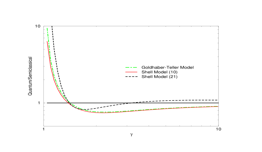
Figure 4: Ratio of the full quantum result to the semi-classical approximation for the cross section of a 20 MeV dipole excitation in ⁴¹Ca by a ¹⁹⁷Au ion. The transition form factors of ⁴¹Ca are described by either the Goldhaber-Teller Model, or by shell-model densities transforming as $(1,0)$ or $(2,1)$ representations of SU(3). As is the case of the calculations summarized in Fig. 3, the cross sections are found to be sensitive to only the leading $\mid$q$\mid$-dependence of the transition form factors and to the relative normalization of the transverse and Coulomb form factors.

In Figs. 3 and 4, we show the ratio of the quantum to semi-classical cross sections for a 20 MeV E1 excitation of a mass 17 and mass 41 targets by ¹⁹⁷Au, using the Goldhaber-Teller and the $(\lambda,\mu$)=(1,0) and (2,1) shell-model transition densities. The Goldhaber-Teller density and the (1,0) shell-model density yield very similar results. The quantum cross section is enhanced relative to the semi-classical cross section for $\gamma$ near unity, it is suppressed at moderate $\gamma$, and returns slowly to the semi-classical result as $\gamma$ becomes large. The cross-section ratio for the retarded (2,1) SU(3) transition density is markedly different from that for the (1,0) density, being larger at low $\gamma$, and approaching the semiclassical result from above as $\gamma$ becomes large. At low $\gamma$, the additional enhancement can in part be traced to the additional powers of $|{\bf q}|=\omega_{T}/\beta$ that appear in the form factors, each leading to an enhancement of the cross section by $1/\beta$ relative to the semi-classical result. The shapes of the curves in Figs. 3 and 4 are determined essentially by the leading-order $|\bf q|$-dependence of the transition form factors, and by the relative normalization of the Coulomb and transverse form factors.

While the dipole excitations provide the bulk of the relativistic heavy-ion-induced electromagnetic cross section, quadrupole transitions have been estimated[9] to contribute significantly to the semi-classical cross section at moderate projectile energies. To investigate the sensitivity of the E2 contribution to target structure effects, we once again compare the predictions of the Goldhaber-Teller and shell models. For the E2 transition densities, it proves useful to classify the densities as representations of the SU(3) oscillator symmetry group, and these are listed in Table II. As in the case of the dipole transitions, the SU(3) classification scheme separates the quadrupole form factors into unretarded and retarded linear combinations of the single-particle transitions. There are two SU(3) form factors that contribute to the E2 photon strength in the long-wavelength approximation. The first of these transforms as $(\lambda,\mu)=(1,1)$ and corresponds to transitions within the same major shell, and the second transforms as $(\lambda,\mu)=(2,0)$ and corresponds to transitions across two major shells. The (2,0) transition is the shell-model equivalent of the giant quadrupole resonance. As can be seen from Table II, all other SU(3) quadrupole transitions are of higher order in the long-wavelength limit.

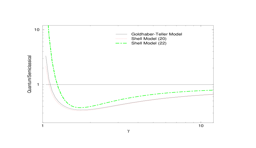
Figure 5: Ratio of the full quantum result to the semi-classical approximation for the cross section of a 20 MeV quadrupole excitation in ⁴¹Ca by a ¹⁹⁷Au ion. The transition form factors for ⁴¹Ca are described by either the Goldhaber-Teller Model, or by shell-model quadrupole densities transforming as $(2,0)$ or $(2,2)$ representations of SU(3). The Goldhaber-Teller transition and the (2,0) SU(3) transition both represent giant quadrupole transitions and involve the same leading $\mid$q$\mid$-dependence in the transition form factors. The (2,2) SU(3) transition corresponds to a retarded transition that does not contribute in leading order in the long-wavelength limit. As in the case of the dipole transitions, the quadrupole cross sections are found to be sensitive only to the leading term in the form factors and to the relative normalization of the transverse and Coulomb form factors.

In Fig. 5, the ratio of the quantum to semi-classical cross sections are shown for a 20 MeV E2 excitation of a mass 41 target by ¹⁹⁷Au, using the (2,0) and (2,2) shell-model form factors, and the quadrupole transition density from the Goldhaber-Teller model. Qualitatively, the results are very similar to what was seen for the dipole cross section. The Goldhaber-Teller and (2,0) transition densities, which have the same behavior in the long-wavelength limit, yield very similar results for the electromagnetic cross section. The retarded (2,2) transition, whose form factors grow more rapidly at small $|{\bf q}|$, shows a more enhanced quantum to semi-classical ratio relative to that seen for the (2,0) and Goldhaber-Teller densities. In all cases, the quantum E2 cross section is reduced dramatically from the semi-classical result for all but the lowest projectile energies, it is enhanced at very small $\gamma$, and returns to the semi-classical result as $\gamma$ becomes large.

No other multipoles contribute measurably to the cross section at relativistic energies. Our studies of the sensitivity of the cross-section to the shape of the form factor show that only the leading-order $|{\bf q}|$-dependence and relative normalization of the transverse and Coulomb transition densities are necessary to provide an adequate description of the heavy-ion-induced electromagnetic cross section.

4 Simple Model for Transition Densities, Cross Sections

In this section, we combine the results of the previous sections to parametrize the projectile and target transition densities that incorporate the nuclear structure details necessary to describe adequately the cross section. Our goal is to rewrite the cross section in a form that allows us to extract an “effective photon spectrum” that can be used with real-photon cross section data. This will provide an essentially model-independent prediction for the electromagnetic cross sections in peripheral heavy-ion reaction, that incorporates the corrections for the kinematic and finite-size effects described in the preceding sections.

For the projectile, we have seen that the heavy-ion-induced electromagnetic cross section is sensitive only to the rms charge radius, so we approximate the projectile form factor as

$$F_{P}(q^{2})=1+{q^{2}R_{P}^{2}\over 6}+{\cal O}(q^{4})\,,$$ (6)

with $R_{P}$ the rms charge radius of the projectile.

For the target, we restrict our attention to the “unretarded” transitions, which dominate the real-photon cross sections in the long-wavelength limit. In the previous section, we saw that the form of the heavy-ion cross section was largely determined by the two factors: the leading-order dependence of the transition form factors on the momentum transfer, and the relative normalization of the Coulomb and transverse form factors. For unretarded transitions, this normalization is determined by Siegert’s theorem[24], which builds in the constraints of angular momentum and current conservation. We can express the quantum mechanical Coulomb excitation cross sections in terms of the real photoexcitation cross section using the following long-wavelength approximation for the transition form factors of multipolarity $\ell$:

$$|F_{\ell}^{T}({\bf q})|^{2} = {\omega_{T}\sigma_{\gamma}(\omega_{T})\over\pi\alpha\rho(\omega_{T})}\times\Big{(}{{\bf q}^{2}\over\omega_{T}^{2}}\Big{)}^{\ell-1}$$

$$|F_{\ell}^{C}({\bf q})|^{2} = {\omega_{T}\sigma_{\gamma}(\omega_{T})\over\pi\alpha\rho(\omega_{T})}\times{\ell\over\ell+1}\Big{(}{{\bf q}^{2}\over\omega_{T}^{2}}\Big{)}^{\ell}\,,$$ (7)

Here $\sigma_{\gamma}(\omega_{T})$ is the cross section for exciting the target with a real photon of energy $\omega_{T}$.

Inserting these expressions into Eq. 2 allows the integrations over the momentum of the virtual photon to be performed explicitly. Since the transition densities are proportional to $\sigma_{\gamma}(\omega_{T})$, the cross section takes the form

$$\sigma_{HI}=\int d\omega_{T}\sigma_{\gamma}(\omega_{T})n_{E\ell}(\omega_{T})\,,$$ (8)

where the effective photon spectrum, $n_{E\ell}(\omega_{T})$, plays the same role as the virtual photon spectrum in the classical calculation. For E1 transitions we find,

$$n_{E1}(\omega_{T})=\frac{2Z_{P}^{2}\alpha}{\pi\omega_{T}\beta^{2}}\left[\ln\left({\Lambda\beta\gamma\over\omega_{T}}\right)\left(1+{1\over 3}\left({\omega_{T}R_{P}\over\gamma}\right)^{2}\right)-{\beta^{2}\over 2}+{\omega_{T}^{2}\over 2\gamma^{2}\Lambda^{2}}-{\Lambda^{2}R_{P}^{2}\over 6}\right],$$ (9)

where $\Lambda^{2}=q_{max}^{2}+({\omega_{T}\over\gamma\beta})^{2}$.

For E2 transitions the improved effective photon spectrum is given by,

$$n_{E2}(\omega_{T}) = \frac{2Z_{P}^{2}\alpha}{\pi\omega_{T}\beta^{2}}\left[\ln\left({\Lambda\beta\gamma\over\omega_{T}}\right)\left(\beta^{2}+{1\over 3}\left({\omega_{T}R_{P}\over\gamma}\right)^{2}\right)-{\beta^{2}\over 2}+{\omega_{T}^{2}\over 2\gamma^{2}\Lambda^{2}}\right.$$ (10)

$$\left.+{2\over 3}{\Lambda^{2}\over\omega_{T}^{2}}\left(1-{\omega_{T}^{2}R_{P}^{2}\over 6}+{3\over 4}{\omega_{T}^{2}R_{P}^{2}\over\gamma^{2}}\right)-{((\Lambda^{2}+{\omega_{T}^{2}\over\beta^{2}})^{2}-({\omega_{T}\over\beta})^{4})R_{P}^{2}\over 9\omega_{T}^{2}}\right].$$

To test our approximations we have recalculated the cross-section ratios appearing in Figs. 2-5 and found that the simplified expressions appearing above reproduce the results of the full calculation.

5 Comparison with Data

In Ref. [10], a crude estimate of the heavy-ion-induced electromagnetic cross section was made by assuming that all of the E1/E2 strength was concentrated in a discrete state at the peak of the giant resonance energy. While this led to a cross section that was significantly lower than that obtained with the corresponding semi-classical calculation, the results were still larger than data. When the finite width of the giant resonance is taken into account, the semi-classical prediction for the heavy-ion cross section is reduced. A similar reduction was expected in the fully quantum-mechanical cross section in reference 10, but a quantitative comparison with data could not be performed without resorting to unjustified assumptions concerning the effects of nuclear structure. The central result of the present work is that with a few simplifying assumptions, it is now feasible to calculate the heavy-ion-induced cross section in exactly the same manner as one does semi-classically.

We focus our attention on the data of Hill et al. [18] for single-neutron removal, leaving a consideration of all the data for a later effort. The advantage of this particular data set is that the cross section for each target is studied with several projectiles, simplifying the search for systematic effects. The total single-neutron-removal cross section, including a component produced by strong interactions in grazing collisions, was measured for each projectile-target combination. In order to extract the electromagnetic cross section, it is necessary first to subtract the strong interaction contribution. For light projectiles, the extracted electromagnetic cross section is sensitive to the method used in estimating the strong contribution. Tables III and IV list the data sets for the electromagnetic contribution to the single-neutron-removal cross section for ¹⁹⁷Au and ⁵⁹Co targets. The cross sections accounting for the strong interaction contribution obtained from the limiting fragmentation scheme of Ref. [20] and from the Glauber estimate of Ref. [12] are listed in columns four and five of the tables, respectively.

Also shown in Tables III and IV are theoretical predictions for the cross sections obtained with the semi-classical equivalent photon flux and with the effective photon fluxes derived in the last section. The cross section is given by

$$\sigma_{HI}=\int_{\omega_{thresh}}^{\omega_{max}}d\omega_{T}[n_{E1}(\omega_{T})\sigma_{E1}^{\gamma}(\omega_{T})+n_{E2}(\omega_{T})\sigma_{E2}^{\gamma}(\omega_{T})]\,,$$ (11)

where $\omega_{thresh}$ is the threshold for single-neutron removal from the target (8(11) MeV for Au(Co)), $\omega_{max}$ is an upper limit for the integration, taken to be 50 MeV, $n_{E\ell}$ are photon fluxes, and $\sigma_{E\ell}^{\gamma}$ are the cross sections for single-neutron removal by a real photon of the indicated multipolarity.

To separate the E1 and E2 contributions to the total photo-neutron cross section, we assumed that the E2 cross section is dominated by the isoscalar giant quadrupole resonance, and is described by[9]

$$\sigma_{E2}^{\gamma}(\omega)={\sigma_{EWSR}\,\omega^{2}\over 1+(\omega^{2}-\omega_{GQR}^{2})^{2}/\omega^{2}\Gamma^{2}}\,,$$ (12)

where $\sigma_{EWSR}=f{0.22ZA^{2/3}\over\pi\Gamma/2}$ $\mu$b-MeV^-1, $\omega_{GQR}$ is the energy of the giant quadrupole resonance, $\Gamma$ is the resonance width, and $f$ is the fractional saturation of the energy-weighted sum rule. Values for these parameters were taken from Ref. [9].

For convenience, the total cross sections $(\sigma_{E1}^{\gamma}+\sigma_{E2}^{\gamma})$ for single-neutron removal were not taken directly from data, but were calculated from the parametrizations of Berman[19]. These parametrized fits overestimate the total photo-neutron cross-sections, which in turn leads to an overestimate of the calculated heavy-ion cross sections. The size of this effect can be estimated by comparing the semi-classical predictions obtained using the parametrized fits with those of reference 9, where the photo-neutron data were used directly. This indicates use of the parametrized fits leads to heavy-ion cross sections that are larger by about $5\%$ for Au and by about 10$\%$ for Co.

The predictions for the Coulomb-excitation cross section, using both the semi-classical and quantum expressions for the equivalent-photon fluxes, are listed in Table III for the Au targets and in Table IV for the Co target. The quantum calculation provides a significantly improved description of the data, particularly if the Glauber picture is used to estimate the strong interaction contribution to the cross section.

6 Summary

We have examined the sensitivity of heavy-ion-induced electromagnetic cross sections to the structure of the target and projectile nuclei. For typical transitions, we have shown that the cross section is only mildly dependent on the projectile charge radius, and more sensitive to the leading $|{\bf q}|$ dependence and the relative normalization of the target’s Coulomb and transverse form factors.

Using these results, we extracted a new equivalent-photon spectra for E1 and E2 transitions, based on the fully-quantum-mechanical cross section derived in Ref. [10]. The new spectra may be used in the same fashion as their semi-classical counterparts to obtain model-independent predictions for electromagnetic processes in relativistic-heavy-ion collisions. Moreover, the new spectra provide an explanation for some anomalously small measured cross sections in terms of single-photon exchange, and leave little room for more exotic multi-photon mechanisms required to explain these cross sections in a semi-classical analysis[20, 21].

Acknowledgements

The work of C.B. and J.F. was performed under the auspices of the U.S. Department of Energy. One of us(C.B.) gratefully acknowledges the support of the Iowa Space Grant Cooperative and the hospitality of the Physics Department of the Univ. of Northern Iowa during the final stages of this work.

Appendix

In this appendix we discuss the shell-model transition form factors and their classification under the SU(3) scheme. We also discuss the use of the continuity equation for the relative normalizations of the Coulomb and transverse form factors.

The Coulomb and the electric transverse form factors for a transition of multipolarity J are defined in terms of the nuclear charge and current transition densities as:

$$F^{C}_{J}(q)=\mbox{\small$\sqrt{\frac{4\pi}{Z^{2}}\frac{2J_{f}+1}{2J_{i}+1}}$}\int_{0}^{\infty}\rho_{J}(r)j_{J}(qr)r^{2}dr$$

$$F^{E}_{J}(q)=\mbox{\small$\sqrt{\frac{4\pi}{Z^{2}}\frac{J+1}{2J+1}}$}\int_{0}^{\infty}\rho_{J,J-1}(r)j_{J-1}(qr)r^{2}dr+\mbox{\small$\sqrt{\frac{4\pi}{Z^{2}}\frac{J}{2J+1}}$}\int_{0}^{\infty}\rho_{J,J+1}(r)j_{J+1}(qr)r^{2}dr\;,$$ (13)

The transition charge and current densities are defined in terms of the reduced matrix elements of the charge and current operators as:

$$\rho_{J}(r)=\int<J_{f}\mid\mid\rho(\mbox{\boldmath$r$})Y_{J}(\hat{\mbox{\boldmath$r$}})\mid\mid J_{i}>\;d\hat{\mbox{\boldmath$r$}}$$

$$\rho_{J,J^{\prime}}(r)=\int<J_{f}\mid\mid\mbox{\boldmath$J(r)\,\cdot\,Y$}\!_{JJ^{\prime}1}(\hat{\mbox{\boldmath$r$}})\mid\mid J_{i}>d\hat{\mbox{\boldmath$r$}}\,.$$ (14)

Donnelly and Haxton[17] have derived expressions for the single-particle matrix elements of the electromagnetic operators that can be used with one-body density-matrix elements (OBDMEs) defined in jj-coupling. The form factors appropriate to SU(3) coupling are linear combinations of these. They can be obtained by expanding the SU(3) OBDMEs in terms of the jj-OBDMEs. For this, we write

$$<J_{f}T_{f}\mid\mid[a^{+}_{(Q_{1}0)}\tilde{a}_{(0Q_{2})}]^{(\lambda\mu)\kappa(\Delta L\Delta S)\Delta J\Delta T}\mid\mid J_{i}T_{i}>=\qquad\qquad\qquad\qquad\qquad$$

$$\sum_{\ell_{1}\ell_{2}}(-)^{Q_{2}}<(Q_{1}0)\ell_{1}(\overline{0Q_{2}})\ell_{2}\|(\lambda\mu)\kappa L>\sum_{j_{1}j_{2}}\left(\begin{array}[]{ccc}\ell_{1}&\frac{1}{2}&j_{1}\\ \ell_{2}&\frac{1}{2}&j_{2}\\ \Delta L&\Delta S&\Delta J\end{array}\right)<f\|(a^{+}_{j_{1}}\tilde{a}_{j_{2}})^{\Delta J\Delta T}\|i>\,,$$

where the unitary 9-J symbol is that equal to the 9-J symbol of Brink and Satchler[22] multiplied by $\hat{j_{1}}\hat{j_{2}}\hat{\Delta L}\hat{\Delta S}$ with $\hat{j}=\sqrt{2j+1}$. The SU(3)$\subset$R(3) Clebsch-Gordon coefficient is that of Draayer and Akiyama[23], and the reduced matrix elements are defined by Brink and Satchler.

Tables I and II list the resulting SU(3) form factors for dipole and quadrupole transitions that do not involve spin-flip, i.e., $\Delta S=0$. For the dipole form factors we consider dipole transitions across one ($\Delta\hbar\omega_{0}=1)$ and across three($\Delta\hbar\omega_{0}=3)$ oscillator shells, and in the case of the quadrupole form factors we consider in-shell ($\Delta\hbar\omega_{0}=0)$ transitions and transitions across two shells ($\Delta\hbar\omega_{0}=2$). As can be seen from the tables, the SU(3) classification corresponds to a separation of the shell-model densities into an unretarded transition and into a set of transitions that are retarded to various orders in ${\bf q}^{2}$. The unretarded dipole form factor transforms as $(\lambda,\mu)=(1,0)$, and contains all the dipole photon strength in the long-wavelength approximation. For the quadrupole transitions there are two unretarded form factors corresponding to $\Delta\hbar\omega_{0}=0$ and $\Delta\hbar\omega_{0}=2$ transitions, and these transform as (1,1) and (2,0) under SU(3), respectively.

In determining the relative normalizations of the Coulomb and transverse form factors it is important to ensure that the continuity equation is satisfied. The continuity equation relates the transition current densities $\rho_{J,J-1}$ and $\rho_{J,J+1}$ to the transition charge density $\rho_{J}$ by:

$$\mbox{\small$\sqrt{\frac{J}{2J+1}}$}\;q\int_{0}^{\infty}\rho_{J,J-1}(r)j_{J-1}(qr)r^{2}dr$$

$$= \frac{\omega_{T}}{c}\int_{0}^{\infty}\rho_{J}(r)j_{J}(qr)r^{2}dr+\mbox{\small$\sqrt{\frac{J+1}{2J+1}}$}\;q\int_{0}^{\infty}\rho_{J,J+1}(r)j_{J+1}(qr)r^{2}dr\,.$$

Thus, the transverse electric form factor can be expressed in terms of the Coulomb form factor and the current densities $\rho_{J,J+1}$ as:

$$F^{E}_{J}(q^{2})=\frac{\omega_{T}}{c\;q}\mbox{\small$\sqrt{\frac{J+1}{J}}$}F^{C}_{J}+\mbox{\small$\sqrt{\frac{2J+1}{J}}$}\int_{0}^{\infty}\rho_{J,J+1}(r)j_{J+1}(qr)r^{2}dr\;.$$ (16)

Alternatively, one could eliminate the current density $\rho_{J,J+1}(r)$, and express $F^{E}_{J}$ in terms of $F^{C}_{J}$ and $\rho_{J,J-1}(r)$.

For the $(\lambda,\mu$)=(1,0) dipole and (1,1) and (2,2) quadrupole transitions the integral involving the transition current $\rho_{J,J+1}$ is identically zero. Thus, the relative normalization of the Coulomb and electric transverse form factors are the same as for the Goldhaber-Teller transitions (Eq. 5). For the retarded transitions the situation is more complicated, and the relation between $F^{T}_{\ell}$ and $F^{C}_{\ell}$ generally depends on $(\lambda,\mu)$. For harmonic-oscillator wave functions of oscillator frequency $\omega_{0}$, the integral $\int^{\infty}_{0}\rho_{J,J+1}\;j_{J+1}\;r^{2}dr$ is proportional to $\frac{\omega_{0}}{c\;q}\int^{\infty}_{0}\rho_{j}\;j_{J}\;r^{2}dr$, and the constants of proportionality are given in Tables I and II. Note that Eq. (17) implies that only one of two distinct combinations of current terms can be written in terms of the charge density[24]. The remaining term is determined by different physics, and in our model this term is distinguished by $\omega_{0}$ rather than $\omega_{T}$.

• Table Captions

• Table I Shell-model form factors for dipole transitions in the SU(3) classification scheme. The form factors are expressed in terms of the variable $y=(b$q/2)², where $b$ is the oscillator parameter. $\hbar\omega_{T}$ is the transition energy and $\hbar\omega_{0}$ is the oscillator energy (i.e., $b=\sqrt{\frac{\hbar}{m\omega_{0}}}$). These form factors correspond to linear combinations of the usual jj-coupled transition form factors. As can be seen from the tables the SU(3) classification separates the transitions into an unretarded transition transforming as $(\lambda,\mu)$=(1,0), and into a set of transitions that are retarded to various orders in ${\bf q}^{2}$.

• Table II Shell-model form factors for quadrupole transitions in the SU(3) classification scheme.

• Table III Comparison of the single-neutron-removal cross section calculated semi-classically with the fully quantum-mechanical photon spectrum derived in the text with data on ¹⁹⁷Au targets.

• Table IV Comparison of the single-neutron removal cross section calculated semi-classically with the fully quantum-mechanical photon spectrum derived in the text with data on ⁵⁹Co targets.

Table I
Dipole Form Factors $\Delta J=1^{-}\,(\Delta L=1\,\Delta S=0)$
$Q_{1}\rightarrow Q_{2}$	($\lambda,\mu)$	FCoul	FT/FCoul
$\Delta\hbar\omega=1\hbar\omega$
$p\rightarrow s$	(1,0)	$\sqrt{\frac{2}{3}}y^{1/2}e^{-y}$	$\frac{\sqrt{2}\omega_{T}}{c\>q}$
$sd\rightarrow p$	(1,0)	$\sqrt{\frac{8}{3}}y^{1/2}(1-\frac{1}{2}y)e^{-y}$	$\frac{\sqrt{2}\;\omega_{T}}{c\>q}$
	(2,1)	- $\sqrt{\frac{2}{15}}y^{3/2}e^{-y}$	$\frac{\sqrt{2}\;\omega_{T}}{c\>q}-\frac{4\sqrt{2}\;\omega_{0}}{c\>q}$
$pf\rightarrow sd$	(1,0)	$\sqrt{\frac{20}{3}}y^{1/2}(1-y+\frac{1}{5}y^{2})e^{-y}$	$\frac{\sqrt{2}\;\omega_{T}}{c\>q}$
	(2,1)	$-\sqrt{\frac{4}{5}}y^{3/2}(1-\frac{1}{3}y)e^{-y}$	$\frac{\sqrt{2}\;\omega_{T}}{c\>q}-\frac{4\sqrt{2}\;\omega_{0}}{c\>q}$
	(3,2)	$-\frac{2\sqrt{2}}{3\sqrt{35}}y^{5/2}e^{-y}$	$\frac{\sqrt{2}\;\omega_{T}}{c\>q}+\frac{2\sqrt{2}\;\omega_{0}}{c\>q}$
$sdg\rightarrow pf$	(1,0)	$\sqrt{\frac{40}{3}}y^{1/2}(1-\frac{3}{2}y+\frac{3}{5}y^{2}-\frac{1}{15}y^{3})e^{-y}$	$\frac{\sqrt{2}\omega_{T}}{c\>q}$
$\Delta\hbar\omega_{0}=3\hbar\omega_{0}$
$pf\rightarrow s$	(3,0)	$\sqrt{\frac{4}{135}}y^{3/2}e^{-y}$	$\frac{\sqrt{2}\omega_{T}}{c\>q}-\frac{2\sqrt{2}\omega_{0}}{c\>q}$
$sdg\rightarrow p$	(3,0)	$\sqrt{\frac{8}{5}}y^{3/2}(1-\frac{1}{3}y)e^{-y}$	$\frac{\sqrt{2}\omega_{T}}{c\>q}-\frac{2\sqrt{2}\omega_{0}}{c\>q}$
	(4,1)	$\frac{2}{3\sqrt{35}}y^{5/2}$	$\frac{\sqrt{2}\omega_{T}}{c\;q}-\frac{8\sqrt{2}\omega_{0}}{c\>q}$

Table II
Quadrupole Form Factors $\Delta J=2^{+}(\Delta L=2\Delta S=0)$
$Q_{1}\rightarrow Q_{2}$	($\lambda,\mu)$	FCoul	F${}^{T}/F^{Coul}$
$\Delta\hbar\omega_{0}=0$
$p\rightarrow p$	(1,1)	$-\sqrt{\frac{8}{15}}ye^{-y}$	$\sqrt{\frac{3}{2}}\frac{\omega_{T}}{c\>q}$
$sd\rightarrow sd$	(1,1)	$\sqrt{\frac{8}{3}}y(1-\frac{2}{5}y)e^{-y}$	$\sqrt{\frac{3}{2}}\frac{\omega_{T}}{c\>q}$
	(2,2)$\kappa=0$	$-\sqrt{\frac{8}{1365}}y^{2}e^{-y}$	$\sqrt{\frac{3}{2}}\frac{\omega_{T}}{c\>q}+\frac{7\sqrt{6}\omega_{0}}{c\>q}$
	(2,2)$\kappa=2$	$\sqrt{\frac{8}{325}}y^{2}e^{-y}$	$\sqrt{\frac{3}{2}}\frac{\omega_{T}}{c\>q}-\frac{5\sqrt{2}}{\sqrt{3}}\frac{\omega_{0}}{c\>q}$
$pf\rightarrow pf$	(1,1)	$-\sqrt{8}y(1-\frac{4}{5}y+\frac{2}{15}y^{2})e^{-y}$	$\sqrt{\frac{3}{2}}\frac{\omega_{T}}{c\>q}$
	(2,2)$\kappa=0$	$-\sqrt{\frac{8}{195}}y^{2}(1-\frac{2}{7}y)e^{-y}$	$\sqrt{\frac{3}{2}}\frac{\omega_{T}}{c\>q}+\frac{7\sqrt{6}\omega_{0}}{c\>q}$
	(2,2)$\kappa=2$	$\frac{2\sqrt{14}}{5\sqrt{13}}y^{2}(1-\frac{2}{7}y)e^{-y}$	$\sqrt{\frac{3}{2}}\frac{\omega_{T}}{c\>q}-\frac{5\sqrt{2}}{\sqrt{3}}\frac{\omega_{0}}{c\>q}$
	(3,3)	$\frac{8}{21\sqrt{15}}y^{3}e^{-y}$	$\sqrt{\frac{3}{2}}\frac{\omega_{T}}{c\>q}\par$
$\Delta\hbar\omega_{0}=2$
$sd\rightarrow s$	(2,0)	$\sqrt{\frac{4}{15}}ye^{-y}$	$\sqrt{\frac{3}{2}}\frac{\omega_{T}}{c\>q}$
$pf\rightarrow p$	(2,0)	$\sqrt{\frac{4}{3}}y(1-\frac{2}{5}y)e^{-y}$	$\sqrt{\frac{3}{2}}\frac{\omega_{T}}{c\>q}$
	(3,1)	$-\frac{4}{5\sqrt{7}}y^{2}e^{-y}$	$\sqrt{\frac{3}{2}}\frac{\omega_{T}}{c\>q}-\frac{5\sqrt{6}}{3}\frac{\omega_{0}}{c\>q}$

Table III
Projectile(Energy/nucleon)	$\sigma_{HI}$(mb)
	Classical	Quantum	Expt.(Lim. Frag.)	Expt.(Glauber)
12C(2.1 GeV)	48	40	75$\pm$14	51$\pm$ 7
20Ne(1.7 GeV)	117	96	151$\pm$13	107$\pm$ 13
20Ne(2.1 GeV)	125	105	153$\pm$18	133$\pm$ 11
40Ar(1.9 GeV)	352	288	348$\pm$34	315$\pm$ 30
56Fe(1.9 GeV)	684	553	601$\pm$54	552$\pm$ 52
86K(1.0 GeV)	1001	762	820$\pm$62	793$\pm$ 62
139La(1.26 GeV)	2472	1886	1970$\pm$130	1952$\pm$ 130
197Au(1.0 GeV)	3967	2912	3077$\pm$200	3066$\pm$200
209Bi(1.0 GeV/nuc)	4211	3154	3244$\pm$205	3233$\pm$205
238U(0.96 GeV/nuc)	5024	3630	3160$\pm$230	3248$\pm$210

Table IV
Projectile(Energy/nucleon)	$\sigma_{HI}$(mb)
	Classical	Quantum	Expt.(Lim. Frag.)	Expt.(Glauber)
12C (2.1 GeV)	9	8	6$\pm$9	-5$\pm$ 5
20Ne(2.1 GeV)	23	20	32$\pm$11	30$\pm$ 7
56Fe(1.9 GeV)	122	98	88$\pm$14	72$\pm$ 9
139La(1.26 GeV)	413	304	302$\pm$40	304$\pm$ 40

References

- [1] G. Baur and H. Rebel, J. Phys. G20, 1 (1994), and references therein.
-
[2]
K. Ieki et al., Phys. Rev. Lett. 70, 6 (1993);
D. Sackett et al., Phys. Rev. C48, 118 (1993);
T. Nakamura et al., Phys. Lett. B331, 296 (1994). - [3] W.J. Llope and P. Braun-Munzinger, Phys. Rev. C45, 799 (1992).
-
[4]
E. Fermi, Z. Phys. 29, 315 (1924);
C.F. Weizsäcker, Z. Phys, 88, 612 (1934);
E.J. Williams, Phys. Rev. 45, 729 (1934). - [5] T. Motobayashi et al., Phys. Rev. Lett. 73, 2680 (1994).
- [6] R. Jäckle and H. Pilkuhn, Nucl. Phys. A247, 521 (1975).
-
[7]
K. Alder and A. Winther, Electromagnetic Excitation,
North-Holland, 1975;
A. Goldberg, Nucl. Phys. A420, 636 (1984). - [8] I.Y. Pomeranchuk and I.M. Shmushkevitch, Nucl. Phys. 23, 452 (1961).
-
[9]
C.A. Bertulani and G. Baur, Phys. Rep. 163, 299 (1984);
W.J. Llope and P. Braun-Munzinger, Phys. Rev. C41, 2644 (1990);
J.W. Norbury, Phys. Rev. C41, 372 (1990);
J.W. Norbury, Phys. Rev. C42, 711 (1990);
C.J. Benesh, Phys. Rev. C46, 2635 (1992). - [10] C.J. Benesh and J.L. Friar, Phys. Rev. C48, 1285 (1993).
- [11] C.J. Benesh and J.L. Friar, Phys. Rev. C50, 3167 (1994).
- [12] C.J. Benesh, B.C. Cook, and J.P. Vary, Phys. Rev. C40, 1198 (1989).
- [13] T. de Forest Jr. and J.D. Walecka, Adv. Phys. 15, 1 (1966).
- [14] D.J. Millener, Unpublished.
- [15] J.P. Elliott, Proc. Roy. Soc. A245, 128 (1958); ibid., A245, 562 (1958).
- [16] M. Harvey, Advances in Nuclear Physics 1, 67 (1968).
- [17] T.W. Donnelly and W.C. Haxton, Atomic Data and Nuclear Data Tables 23, 103 (1979); ibid., 25, 1 (1980).
-
[18]
J.C. Hill et al., Phys. Rev. C39, 524 (1989);
M.T. Mercier, J.C. Hill, F.K. Wohn, and A.R. Smith, Phys. Rev. Lett. 52, 898 (1984);
M.T. Mercier et al., Phys. Rev. C33, 1655 (1986);
J.C. Hill, F.K. Wohn, J.A. Winger, and A.R. Smith, Phys. Rev. Lett. 60, 999 (1988);
A.R. Smith, J.C. Hill, J.A. Winger, and P.J. Carol, Phys. Rev. C38, 210 (1988). - [19] B.L. Berman, Atlas of Photo-Neutron Cross Sections, University of California Report No. UCRL-78482.
- [20] J.W. Norbury and G. Baur, Phys. Rev. C48, 1915 (1993).
-
[21]
W.J. Llope and P. Braun-Munzinger, Phys. Rev. C45,
799 (1992);
T. Aumann et al., Phys. Rev. C47, 1728 (1993). - [22] D. M. Brink and G.R. Satchler, Angular Momentum (Clarendon, Oxford, 1968).
- [23] J.P. Draayer and Y. Akiyama, J. Math. Phys. 14, 1904 (1973); Y. Akiyama and J.P. Draayer, Comput. Phys. Comm. 5, 5 (1973).
- [24] J.L. Friar and S. Fallieros, Phys. Rev. C29, 1645 (1984).
-