THE “HOLE” IN HELIUM

Abstract

The measurement and analysis of electron scattering from ³He and ⁴He by Sick and collaborators reported 20 years ago remains a matter of current interest. By unfolding the measured free-proton charge distribution, they deduced a depression in the central point nucleon density, which is not found in few-body calculations based on realistic potentials. We find that using wave functions from such calculations we can obtain good fits to the He charge distributions under the assumption that the proton charge size expands toward the center of the nucleus. The relationship to 6-quark Chromo-Dielectric Model calculations, is discussed. The expansion is larger than than the predictions of mean field bag calculations by others or our CDM calculations in the independent pair approximation. There is interest here in the search for a “smoking gun” signal of quark substructure.

I INTRODUCTION

The charge distribution of nuclei has been the subject of experimental studies for more than forty years. Electron scattering and muonic atoms now provide detailed descriptions of the full range of stable, and many unstable nuclides. Unique among the nuclides are the isotopes ³He and ⁴He because they exhibit a central density about twice that of any other nuclide. There is a long-standing apparent discrepancy between the experimentally extracted charge distributions and detailed theoretical structure calculations which include only nucleon degrees of freedom.

McCarthy, Sick and Whitney[1, 2] performed electron scattering experiments on these isotopes up to momentum transfers of 4.5 fm^-1 yielding a spatial resolution of $~{}0.3$ fm. They extract a “model independent” charge distribution, which means that their analysis of the data is not based upon any assumed functional form for the charge distributions. Their charge distributions are shown in Fig. 1. Taken alone, they do not appear to be extraordinary. However, using a finite proton form factor, which fits the experimentally measured rms radius of about 0.83 fm, they unfolded the proton structure from the charge distributions to obtain the proton point distributions. For both isotopes there is a significant central depression of about 30% extending to about 0.8 fm. Sick[2] also presented results where relativistic and meson effects are included. These are shown for ⁴He in Fig. 2. One note of caution here is that it is not possible to subtract these effects from the experimental data in a completely model-independent way.

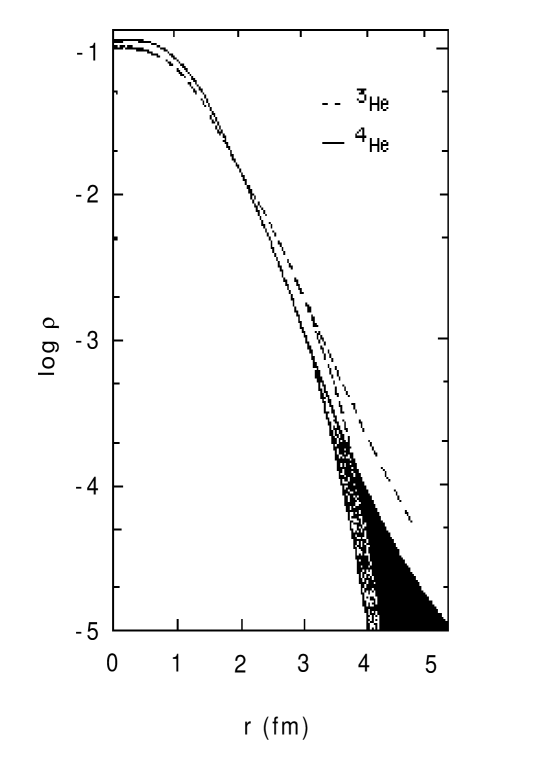
FIG. 1.: Model-independent charge distributions extracted from experiment. Reproduced from McCarthy et al.[1].

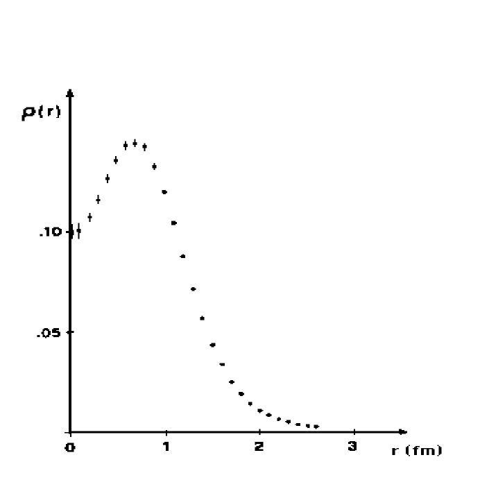
FIG. 2.: Point-proton density distributions obtained by unfolding the finite free proton form factor, allowing for meson exchange corrections and relativistic effects. Reproduced from Sick[2].

One might assume that such a central depression is to be expected because of the short-range repulsion of the nucleon-nucleon interaction. So far, this is not borne out by numerous detailed theoretical calculations, none of which finds a significant central depression, certainly not of the above magnitude. Relatively smaller central depressions are found in Green’s function Monte Carlo (GFMC) calculations of the alpha particle for realistic models of the two- and three-nucleon interaction. (see Fig. 4 below.)

The status of theoretical structure calculations through mass number 4 is very satisfactory at present. Given any assumed interaction, the few body problem can be solved to within tenths of an MeV in energy and the wave function can be calculated to a precision better than that required for the present discussion.

In using a nuclear wave function to construct a charge distribution, one must assume a nucleon charge density and the possibility of meson exchange contributions. While the meson exchange contributions in the transverse channel are well-constrained (at least at moderate momentum transfer) by current conservation, no such constraint is available in the longitudinal channel. Indeed, meson exchange current contributions are of relativistic order and hence one must be careful when interpreting them with non-relativistic wave functions.

Given these caveats, it is possible to reproduce reasonably well the longitudinal form factors of 3- and 4-body nuclei within a nucleons plus meson-exchange model.[3, 4] The current and charge operators are constructed from the N-N interaction and required to satisfy current conservation at non-relativistic order. The resulting meson-nucleon form factors are quite hard, essentially point-like.[3] This raises the possibility of explaining the form factors in quark or soliton based models, which would describe the short-range two-body structure of the nucleons in a more direct way than is available through meson exchange current models. For example, see the discussion of a model by Kisslinger et al.[6] below.

We present here a possible explanation of the electric form factors which does not involve a hole in the point-proton density distribution, but rather is consistent with theoretical few body calculations. It involves the variation of the proton charge size as a function of density, or as a function of nucleon-nucleon separation. This is not depicted as an average ‘swelling’ of the nucleon, but as a result of short-range dynamics in the nucleon-nucleon system. The results presented here are preliminary but encouraging.

II QUARK SUBSTRUCTURE OF NUCLEI AND NUCLEONS

Within the context of soliton models, there have been numerous calculations of the nucleon size in nuclear media. Most of these involve immersion of solitons in a uniform (mean) field generated by other nucleons. Another approach has been the 3-quark/6-quark/9-quark bag models, which has been applied to various nuclear properties, including the EMC effect. It has been applied by Kisslinger et al.[6] to the He electric form factors with some success.

In a series of papers, Koepf, Pepin, Stancu and Wilets[5, 7, 8] have studied the 6-quark substructure of the two-nucleon problem, and in particular obtain the variation of the quark wave functions with inter-nucleon separation. Contrary to previous expectations, the united 6-quark cluster does not exhibit a significant decrease in the quark momentum distribution function in spite of an increase in the volume available to the individual quarks.[7] This is due to configuration mixing of higher quark states. Such a momentum decrease was proffered as an explanation of the EMC effect. However, the united cluster does have approximately twice the volume of confinement of each 3-quark cluster, and the quarks extend to a volume nearly three times that of the 3-quark clusters, again enhanced by configuration mixing of excited states.

In Fig. 3 we exhibit the proton rms charge radius $r_{p}$ extracted as follows from the calculations of Pepin et al.[8]: the abscissa gives the effective nucleon-nucleon separation $r_{NN}$ obtained by the Fujiwara transformation; the soliton-quark structure is a 6-quark deformed composite. The proton rms radius is defined to be

$$r_{p}=\sqrt{<r^{2}>-r_{NN}^{2}/4}$$ (1)

where the quark density used in calculating $<r^{2}>=\int\rho_{q}r^{2}d^{3}r$ is the six-quark density normalized to unity.

FIG. 3.: Proton rms charge radius as a function of inter-nucleon separation. The dashed line is a gaussian approximation, normalized to the free value.

For well separated solitons, the $r_{NN}$ is just the separation of the soliton centers and $r_{p}=0.83$ fm as indicated by the horizontal line. Large deformations (near separation) are difficult to calculate so that the figure does not reproduce well the separation region. Shown also in the figure is a gaussian approximation fitted to $r_{NN}=0$, $r_{NN}=1$ fm, and the asymptotic region, see Eq. (5) below, with $A=0.45,\ s=0.92$ fm. Then the charge distribution due to two-body correlations is

$$f_{p}(\mathchoice{{\hbox{\boldmath$\displaystyle r_{i},r_{j};r$}}}{{\hbox{\boldmath$\textstyle r_{i},r_{j};r$}}}{{\hbox{\boldmath$\scriptstyle r_{i},r_{j};r$}}}{{\hbox{\boldmath$\scriptscriptstyle r_{i},r_{j};r$}}})=\Big{\{}\delta_{ip}\ \exp\big{[}-|\mathchoice{{\hbox{\boldmath$\displaystyle r-r_{i}$}}}{{\hbox{\boldmath$\textstyle r-r_{i}$}}}{{\hbox{\boldmath$\scriptstyle r-r_{i}$}}}{{\hbox{\boldmath$\scriptscriptstyle r-r_{i}$}}}|^{2}/b^{2}(r_{ij})\big{]}$$ (2)

$$+\delta_{jp}\ \exp\big{[}-|\mathchoice{{\hbox{\boldmath$\displaystyle r-r_{j}$}}}{{\hbox{\boldmath$\textstyle r-r_{j}$}}}{{\hbox{\boldmath$\scriptstyle r-r_{j}$}}}{{\hbox{\boldmath$\scriptscriptstyle r-r_{j}$}}}|^{2}/b^{2}(r_{ij}\big{]})\Big{\}}/2\,\pi^{3/2}b^{3}(r_{j})$$ (3)

where we assumed and indicate explicitly that $b$ is a function of the distance $r_{ij}$ between the nucleons i and j, as we expand upon later, and that the proton and neutron functions are the same. Here “$p$” stands for “proton” and the Kronecker deltas pick out protons among $i$ and $j$.

Using the independent pair approximation (IPA) and Eq. (2) we find the charge distribution by employing a two-body correlation function $\rho_{2}(\mathchoice{{\hbox{\boldmath$\displaystyle r_{i},r_{j}$}}}{{\hbox{\boldmath$\textstyle r_{i},r_{j}$}}}{{\hbox{\boldmath$\scriptstyle r_{i},r_{j}$}}}{{\hbox{\boldmath$\scriptscriptstyle r_{i},r_{j}$}}})$,

$$\rho_{ch}(r)=\sum_{i<j}\int d^{3}r_{i}\int d^{3}r_{j}\,\rho_{2}(\mathchoice{{\hbox{\boldmath$\displaystyle r_{i},r_{j}$}}}{{\hbox{\boldmath$\textstyle r_{i},r_{j}$}}}{{\hbox{\boldmath$\scriptstyle r_{i},r_{j}$}}}{{\hbox{\boldmath$\scriptscriptstyle r_{i},r_{j}$}}})f_{p}(\mathchoice{{\hbox{\boldmath$\displaystyle r_{i},r_{j};r$}}}{{\hbox{\boldmath$\textstyle r_{i},r_{j};r$}}}{{\hbox{\boldmath$\scriptstyle r_{i},r_{j};r$}}}{{\hbox{\boldmath$\scriptscriptstyle r_{i},r_{j};r$}}})/3\,.$$ (4)

There are six pairs $(i,j)$. Each proton appears three times; Hence the factor 1/3.

III PHENOMENOLOGICAL DENSITY-DEPENDENT PROTON FORM FACTOR

To obtain some qualitative feeling for the expansion of the proton charge size with nucleon density, we assume a proton form factor $f_{p}$ (differing from Eq. (2)) with a size that depends simply on the local density and hence on the distance from the center of the nucleus $(r^{\prime})$. Then

$$\rho_{ch}(r)=\int d^{3}r^{\prime}\rho(r^{\prime})f_{p}(\mathchoice{{\hbox{\boldmath$\displaystyle r,r^{\prime}$}}}{{\hbox{\boldmath$\textstyle r,r^{\prime}$}}}{{\hbox{\boldmath$\scriptstyle r,r^{\prime}$}}}{{\hbox{\boldmath$\scriptscriptstyle r,r^{\prime}$}}})\,,$$ (5)

where $\rho$ is the (theoretical) point proton density

$$f_{p}(\mathchoice{{\hbox{\boldmath$\displaystyle r,r$}}}{{\hbox{\boldmath$\textstyle r,r$}}}{{\hbox{\boldmath$\scriptstyle r,r$}}}{{\hbox{\boldmath$\scriptscriptstyle r,r$}}}^{\prime})=\exp\big{[}-|\mathchoice{{\hbox{\boldmath$\displaystyle r-r$}}}{{\hbox{\boldmath$\textstyle r-r$}}}{{\hbox{\boldmath$\scriptstyle r-r$}}}{{\hbox{\boldmath$\scriptscriptstyle r-r$}}}^{\prime}|^{2}/b^{2}(r^{\prime})\big{]}\ /\pi^{3/2}b^{3}(r^{\prime})$$ (6)

and we choose

$$b(r^{\prime})=b_{0}[1+Ae^{-r^{\prime 2}/s^{2}}]\,,$$ (7)

with $b_{0}=\sqrt{2/3}$ 0.83 fm, the free proton value. A fairly good fit to the data was found with $A=0.45$ and $s=0.65$ fm corresponding to $b(0)$ equal to the central value given in Fig. 3. The best fit, with only slightly better $\chi$-squared, was obtained with $A=2.10$ and $s=0.13$ fm, which does not seem to be reasonable, in that the $A$ is too large and the $s$ too small.

FIG. 4.: ⁴He density distributions including a fit with a variable proton charge size. The dashed curve labelled “Carlson” is based on a Green’s function Monte Carlo calculation [4]

IV THE INDEPENDENT PAIR APPROXIMATION

In the spirit of the independent pair approximation, the charge distribution was calculated using Eq. (3) with $\rho_{2}$ the two-particle correlation function[4]. The proton size parameter $b(r_{12})$ was first taken from the gaussian fit to the calculations of Pepin et al.[8]. The improvement over the free constant proton size, as shown in Fig. 5 (dot-dash) was small.

A phenomenological fit to the data was made with a parameterized $b$ given by

$$b(r_{12})=b_{0}[1+Ae^{-(r_{12}/s)^{n}}]\,,$$ (8)

where $n=2$ is of the gaussian form. $n>2$ yields a sharper transition. Indeed, $n\to\infty$ yields a step function. Recall that the model of Kisslinger et al. corresponds to a step function.

We examined $n$ = 2, 4 and 6. Although the $A$ and $s$ were different in each case, the quality of fits were very similar. The corresponding best fit values of $(A,\ s,\ n)$ for the three $n$’s were (2.185, 0.883, 2), (0.976, 1.245, 4), (0.774, 1.34, 6). In Fig. 5 we show the results for $n$=2 since the others are indistinguishable to the eye. FIG. 5.: ⁴He density distributions constructed from variational point densities and two-body correlation functions in a parameterized variational calculation by Carlson et al.[4]. The curve labelled “Pepin” uses the gaussian fit of Fig. 3, based on the calculations of Pepin et al.[8]. The solid curve is a phenomenological fit as described in the text

V CONCLUSIONS

We have obtained a phenomenological fit to the ⁴He charge distribution by assuming a proton size which increases with increasing density. More specifically, we minimize the charge distribution $\chi$-squared using a two-parameter gaussian function of $r$, the distance from the center-of mass.

We would like to identify the variable proton size with the structure function of Fig. 3 derived from 6-quark $N$-$N$ studies in the spirit of the independent pair approximation. Fairly good agreement with experiment was obtained with a phenomenological parameterization of the proton size function.

The inadequacy of the previous calculation might be due to

$\bullet$ A constant confinement volume was assumed for the six-quark structure as a function of deformation. It may be that the intermediate volume (between separated and united clusters) is larger.

$\bullet$ The independent pair approximation may be invalid at the high densities of the central region.

$\bullet$ Meson effects should be recalculated using the quark structure functions given (say) by the six-quark IPA model.

Items 1 and 3 are topics for further investigation. In addition, one must study the predictions of such models for quasi-elastic scattering. In the quasi-free regime, nucleon models produce a good description of the data as long as realistic nucleon interactions, including charge exchange, are incorporated in the final-state interactions.[9] Unlike the charge form factor, two-body charge operators are expected to play a much smaller role here [4]. The combination of the two regimes provides a critical test for models of structure and dynamics in light nuclei.

VI REFERENCES

REFERENCES

- [1] J. S. McCarthy, I. Sick and R. R. Whitney, Phys. Rev. C 15, 1396 (1977).
- [2] I. Sick, Lecture Notes in Physics, 87, 236 (Springer, Berlin, 1978).
- [3] R. Schiavilla, V. R. Pandharipande, and D. O. Riska, PRC 40, 2294 (1989) .
- [4] R. Schiavilla and D. O. Riska, Phys. Lett. 244B, 373 (1990); R. B. Wiringa, Phys. Rev. C 43, 1585 (1991); J. Carlson, Nucl. Phys. A522, 185c (1991).
- [5] W. Koepf, L. Wilets, S. Pepin and Fl. Stancu, Phys. Rev. C 50, 614 (1994).
- [6] L. S. Kisslinger, W.-H. Ma and P. Hoodbhoy, Nuc. Phys. A459, 645 (1986); W.-H. Ma and L. S. Kisslinger, Nuc. Phys. A531, 493 (1991).
- [7] W. Koepf and L. Wilets, Phys. Rev.C 51, 3445 (1995).
- [8] S. Pepin, Fl. Stancu, W. Koepf and L. Wilets, Phys. Rev. C 53, 1368 (1996).
- [9] J. Carlson and R. Schiavilla, Phys. Rev. Lett. 68, 3682 (1992); Phys. Rev. C49, R2880 (1994).