Using Faddeev Differential Equations to Calculate Three-Body Resonances

Algorithm, based on explicit representations for analytic continuation of the T-matrix Faddeev components on unphysical sheets, is worked out for calculations of resonances in the three-body quantum problem. According to the representations, poles of T–matrix, scattering matrix and Green function on unphysical sheets, interpreted as resonances, coincide with those complex energy values where appropriate truncations of the scattering matrix have zero as eigenvalue. Scattering amplitudes on the physical sheet, necessary to construct scattering matrix, are calculated on the basis of the Faddeev differential equations. The algorithm developed is applied to search for the resonances in the $nnp$ system and in a model three-boson system.

LANL E-print nucl-th/9602001

Published in Phys. Atom. Nucl. 60 No. 2 (1997), 177–185

I Introduction

Resonances are one of most interesting phenomena in scattering of quantum particles. The problem of definition and studying resonances is payed a lot of attention both in physical and mathematical literature (see, e. g., the books [1] – [8]). Main difficulties connected with a rigorous definition of resonance are explicitly emphasized by B. Simon in his survey [9]. A presence of such difficulties is obliged, first of all, to the fact that in a contrast to the usual spectrum, resonances are not an unitary invariant of an operator (Hamiltonian of a quantum system). The generally accepted interpretation of resonance as a complex pole of the scattering matrix continued analytically on unphysical sheet(s) of the energy plane, goes back to the known paper by G. Gamow [10]. For radially symmetric potentials, such an interpretation of the two-body resonances has been rigorously approved by R. Jost [11]. Beginning from E.C. Titchmarsh [12] resonances are considered as well as poles of analytic continuation of the Green function (or its matrix elements between suitable states [6], [7]). A survey of different physical approaches to studying three-body resonances may be found e. g., in [5] and [13].

At the moment, one of the most effective approaches to practical calculation of resonances is the complex scaling method [14] (see also [7], [9]). This method is applicable to the few-body problem in the case where interaction potentials between particles are analytic functions of coordinates. The complex scaling gives a possibility to rotate the continuous spectrum of the $N$-body Hamiltonian in such a way that certain sectors become accessible for observation on unphysical sheets neighboring with the physical one. At the same time, the real discrete spectrum of the Hamiltonian stays fixed during all the scaling transformation. Resonances in the sectors above turn out to be extra discrete eigenvalues of the scaled Hamiltonian [7]. Thereby, when searching for resonances one may use standard methods to find discrete spectrum. Practical applications of the complex scaling method to concrete problems may be found, in particular, in the recent papers [15] – [17]. Alongside with the complex scaling, another methods are used for calculations of three-body resonances which are based in particular on solving the momentum space Faddeev integral equations [18], [19] continued through the cut (see the survey [13] by K. Möller and Yu.V. Orlov and the literature cited therein). In this approach, resonances are searched for as poles of the T-matrix.

The present paper is devoted to developing a method to calculate three-body resonances using the recently found explicit representations disclosing a structure of the T-matrix on unphysical sheets as well as analogous representations for the scattering matrix and resolvent [20], [21]. These representations were obtained in supposition that the interaction potentials were pairwise and falling–off in the coordinate representation not slower than exponentially. According to the representations [20], [21], the matrix ${\bf M}(z)=\{M_{\alpha\beta}(z)\}$, $\alpha,\beta=1,2,3,$ constructed of the operator $T(z)$ Faddeev components [18], [19], is explicitly expressed on unphysical sheet $\Pi_{l}$ of the energy $z$ plane in terms of this matrix itself taken on the physical sheet and a certain truncation $S_{l}(z)$ of the total three-body scattering matrix $S(z)$. Character of the truncation is determined by the index (number) $l$ of the unphysical sheet concerned. Respective representations for analytic continuation of the matrix $S(z)$ and resolvent $R(z)$ follow immediately from the representations for $\left.{\bf M}(z)\right|_{\Pi_{l}}$. A main consequence of the representations admitting direct practical applications, is the fact that the T-matrix and resolvent as well as the scattering matrix have nontrivial singularities on unphysical sheet $\Pi_{l}$ exactly at those values of the energy $z$ where the corresponding matrix $S_{l}(z)$ has zero as eigenvalue. It is important that $S_{l}(z)$ is considered on the physical sheet only. Therefore, one can provide a search for resonances (poles of ${\bf M}(z)$, $S(z)$ and $R(z)$ ) on a certain unphysical sheet $\Pi_{l}$ keeping $z$ always on the physical one and calculating only a position of zeros of the operator-valued function $S_{l}(z)$. For all this, one can use any method allowing to calculate (on the physical sheet) amplitudes of the processes necessary to construct the truncation $S_{l}(z)$.

In the present paper, the matrices $S_{l}(z)$ are computed on the base of the numerical algorithm [22] elaborated to solve the Faddeev differential equations in configuration space (see the book [19], survey [23] and references therein). Certainly, when computing the amplitudes on the physical sheet one has to extend the Faddeev differential formulation of the scattering problem as well on the complex values of $z$. It should be noted that, in the holomorphy domain (see [21]) of the amplitudes, the differential formulation stays to be correct.

Unfortunately, the algorithm [19], [22], [23] (see also [24] –[27]) has been worked out in details only for the processes $(2\longrightarrow 2,3)$. Thus, there may be computed in practice only the amplitudes of elastic scattering and rearrangement for the processes $(2\longrightarrow 2)$ and the breakup amplitude into three particles. A knowledge of these amplitudes is sufficient to compute those truncations $S_{l}(z)$ of the three-body scattering matrix $S(z)$, zeros of which are “responsible” for resonances situated on the so-called two-body unphysical sheets, i. e. those sheets of the energy Riemann surface where the parameter $z$ may be guided going around the pair thresholds only. As a concrete application of the method concerned we make a search for resonances in the $nnp$ system and in a model system of three bosons with the nucleon masses.

Let us describe shortly structure of the paper.

In Sec. II, we introduce main notations and formulate the explicit representations [21] for the unphysical-sheet three-body T-matrix, scattering matrix and resolvent which are used then to approve the numerical method of the work.

In Sec. III the system $nnp$ and a three-boson system are considered. Formulations of the boundary-value problems [19], [22], [23] are given for the Faddeev partial differential equations, corresponding to the processes $(2\longrightarrow 2,3)$ in these systems and going out to a domain of complex energy values in the physical sheet. Numerical method to solve these problems is described. Truncated (partial) scattering matrices are constructed in terms of the amplitudes for elastic scattering $(2\longrightarrow 2)$. Zeros of these matrices represent resonances (including virtual poles) on the unphysical sheet connected with the physical one by crossing the continuous spectrum interval between the deuteron energy and three-body threshold. Results of numerical computations are exposed.

We conclude this introduction with some notation. Throughout the paper, we understand by $\sqrt{z-\lambda}$, $z\in{{\mathbb{C}}}$, $\lambda\in{{\mathbb{R}}}$, the main branch of the function $(z-\lambda)^{1/2}$. By $\hat{p}$ we denote the unit vector in the direction $p\in{{\mathbb{R}}}^{n}$, $\hat{p}=\frac{\textstyle p}{\textstyle|p|}$, and by $S^{n-1}$, the unit sphere in ${{\mathbb{R}}}^{n}$, $\hat{p}\in S^{n-1}$.

II Explicit representations for -matrix, scattering matrix and resolvent on unphysical sheets

The scattering matrix, -matrix and Hamiltonian resolvent (Green function) for a quantum-mechanical system are stringently connected with each other. Therefore, all these three objects, considered as functions of energy, have usually the same Riemann surface. Such a fact takes place at least in the multichannel scattering problem with binary channels and in the three-body problem with quickly decreasing interactions [28], [21]. In a “first approximation”, the structure of the Riemann surfaces in these problems coincides. The thing is that the branching points (in real axis) are stipulated to these surfaces in the both problems by the same reason, namely by a presence of the Cauchy-type integrals in the Lippmann–Schwinger or Faddeev equations. In the equations considered in the momentum representation, the Cauchy-type integrals are engendered by the kernels $\frac{\textstyle\delta(p-p^{\prime})}{\textstyle\lambda+p^{2}-z}$ with $\lambda$, the channel thresholds and $p$, $p\in{{\mathbb{R}}}^{n}$, the respective channel momentum variables. In the case of the channels $(2\longrightarrow 2,3)$ in three-body problem and the odd-dimensional channels (i. e., with $n$ odd) in the matrix multichannel problem, the thresholds $\lambda$ turn out to be the branching points of the second order. Even-dimensional channels in the multichannel problem as well as the channel $(3\rightarrow 2,3)$ in the three-body problem give logarithmic branching points (see [21], [28], [13]).

The method used for calculation of resonances in the present work, is based on the explicit representations [21] for analytic continuation of the T-matrix, scattering matrices and Green function on unphysical sheets keeping true at least for a part of the three-body Riemann surface. To describe this part we introduce the auxiliary vector-function $f(z)=(f_{0}(z)),f_{1,1}(z),...,f_{1,n_{1}}(z),$ $f_{2,1}(z),...,f_{2,n_{2}}(z),$ $f_{3,1}(z),...,f_{3,n_{3}}(z))$    with $\enspace f_{0}(z)$ $=$ $\ln{z}$ and $f_{\alpha,j}(z)$ $=$ $(z-\lambda_{\alpha,j})^{1/2}.$ Here, by $\lambda_{\alpha,j}$ we understand respective bound-state energies of pair subsystems $\alpha,$ $\alpha=1,2,3,$ $j=1,2,...,n_{\alpha},$ numerated taking into account their multiplicities. It is supposed that $n_{\alpha}<\infty$. The sheets $\Pi_{l}$ of the vector-function $f(z)$ Riemann surface $\Re$ are numerated via multi-index $l=(l_{0},l_{1,1},...,l_{1,n_{1}},l_{2,1},...,l_{2,n_{2}},l_{3,1},...,l_{3,n_{3}}),$ where $l_{\alpha,j}=0$ if the sheet $\Pi_{l}$ corresponds to the main (arithmetic) branch of the square root $(z-\lambda_{\alpha})^{1/2}.$ Otherwise, $l_{\alpha,j}=1$ is assumed. Value of $l_{0}$ coincides with the number of branch of the function $\ln{z}$, $\ln z=\ln|z|+i\,2\pi l_{0}+i\phi$ where $\phi=\mathop{\rm arg}z$. For the physical sheet identified by $l_{0}=l_{\alpha,j}=0$, $\alpha=1,2,3,\enspace j=1,2,...,n_{\alpha}$, we use the notation $\Pi_{0}$. A “sticking” of the sheets $\Pi_{l}$ of the surface $\Re$ is realized in intervals between neighboring thresholds along rims of the cut along the continuous spectrum. A detailed description of the surface $\Re$ may be found in [28].

The type $\Re$ surfaces without extra branching points arise in the multichannel problems with binary channels only. Structure of the total three-body Riemann surface is essentially more complicated. For instance, the sheets $\Pi_{l}$ with $l_{0}=\pm 1$ have additional branching points corresponding to resonances of the two-body subsystems. In the sheets $\Pi_{l}$ with $l_{0}=0$, one can discover (in the left half-plane) logarithmic branching points of a kinematical origin. The part $\Re^{(3)}$ of the total three-body Riemann surface where the representations [21] are valid, consists of the surface $\Re$ sheets $\Pi_{l}$ identified by $l_{0}=0$ (such unphysical sheets are called two-body sheets) and two three-body sheets identified by $l_{0}=\pm 1$ and $l_{\alpha,j}=1,$ $\alpha=1,2,3,$ $j=1,2,...,n_{\alpha}.$ Note that $\Re^{(3)}$ includes all the unphysical sheets neighboring with the physical sheet $\Pi_{0}$.

FIG. 1.: Physical, $\Pi_{0}$, and neighboring unphysical, $\Pi_{(0,1)}$, $\Pi_{(1,1)}$ and $\Pi_{(-1,1)}$, sheets of the Riemann surface in the three-nucleon $(nnp)$ and model three-boson problems. The near (in figure) rim of the cut in the sheet $\Pi_{0}$ is identified in the interval between the deuteron energy $E_{d}$ and three-body threshold $z=0$ with the remote rim of the cut in the sheet $\Pi_{(0,1)}$. On the contrary, the remote rim in the sheet $\Pi_{0}$ is identified in this interval with the near rim in the sheet $\Pi_{(0,1)}$. In the interval $(0,+\infty)$, one identifies the near rim of the cut in the sheet $\Pi_{0}$ with the remote rim in the sheet $\Pi_{(1,1)}$. Respectively, the remote rim in the sheet $\Pi_{0}$ is identified in this interval with the near rim in the sheet $\Pi_{(-1,1)}$. On the sheet $\Pi_{(0,1)}$, the virtual level $z_{\rm res}({}^{3}\!{H})$ in the s-state of the $nnp$-system is marked, and the resonance $z_{\rm res}(\mbox{3B})$ in the model three-boson system. Also, the complex conjugate pole $\overline{z}_{\rm res}(\mbox{3B})$ is marked.

In the case of the $nnp$-system and a model three-boson system considered below, the surface $\Re^{(3)}$ is shown schematically in Fig. 1. In this case a single pair threshold, the deuteron energy $\lambda=E_{d}$ is present only. Therefore, the index $l$ of the sheets $\Pi_{l}$ consists of two components only: $l=(l_{0},l_{1})$. In the terminology accepted, the sheet $\Pi_{(0,1)}$ (see Fig. 1) is a two-body sheet, but the sheets $\Pi_{(-1,1)}$ and $\Pi_{(1,1)}$ are three-body ones.

Construction of the representations for the T-matrix consists of the following stages. At the first step, one carries out analytic continuation on unphysical sheets, of the absolute terms and kernels of the Faddeev integral equations for the components $M_{\alpha\beta}(z)$ (the continuation is understood in the sense of distributions). As the absolute terms as the kernels after continuation are expressed in terms of the pair T-matrices and scattering matrices taken on the physical sheet. Transforming the Faddeev equations continued, one finds the kernels $\left.M_{\alpha\beta}(P,P^{\prime},z)\right|_{z\in\Pi_{l}}$ can be explicitly expressed in terms of these kernels themselves taken on the physical sheet $\Pi_{0}$ in their off-shell and/or half-on-shell variants. It is supposed in the last case that the first argument $P$ of the kernels $\left.M_{\alpha\beta}(P,P^{\prime},z)\right|_{z\in\Pi_{l}}$ is taken on the energy (“mass”) shells $|P|^{2}=z$ or $|p_{\alpha}|^{2}=z-\lambda_{\alpha,j},$ $j=1,2,...,n_{\alpha}.$ Here, we use the notations $P=\{k_{\alpha},p_{\alpha}\}$ with $k_{\alpha},p_{\alpha},$ $\alpha=1,2,3,$ standing for the standard relative momenta [19]. Transferring in the expressions obtained all the off-shell terms to the l.h. part and inverting an operator arising there, one comes to a closed system of equations for the half-on-shell components $\left.M_{\alpha\beta}(P,P^{\prime},z)\right|_{z\in\Pi_{l}}$. This system admits an explicit solution using the terms of the physical sheet only. As a result one gets the following representations for the matrix ${\bf M}(z)=\left\{M_{\alpha\beta}(z)\right\},\alpha,\beta=1,2,3,$ continued on the sheet $\Pi_{l}$:

$$\left.{\bf M}(z)\right|_{\Pi_{l}}={\bf M}(z)-{\bf B}^{\dagger}(z)A(z)LS_{l}^{-1}(z)\tilde{L}{\bf B}(z).$$ (1)

Here, the factor $A(z)$ is the diagonal matrix,

$$A(z)={\rm diag}\{A_{0}(z),A_{1,1}(z),...,A_{1,n_{3}}(z)\},$$

combined of the functions $A_{0}(z)=-\pi iz^{2}$ and $A_{\alpha,j}=-\pi i\sqrt{z-\lambda_{\alpha,j}}.$ Notations $L$ and $\tilde{L}$ are used for diagonal number matrices whose nontrivial elements are the sheet $\Pi_{l}$ indices:

$$L={\rm diag}\{l_{0},l_{1,1},...,l_{3,n_{3}}\}\,\,\mbox{\rm and}\,\,\,\tilde{L}={\rm diag}\{|l_{0}|,l_{1,1},...,l_{3,n_{3}}\}.$$

By $S_{l}(z)$ we understand a truncation of the three-body scattering matrix: $S(z)$,   $S(z):\,\hat{\cal G}\rightarrow\hat{\cal G},$    $\hat{\cal G}=L_{2}(S^{5})\mathop{\oplus}\limits_{\alpha=1}^{3}\mathop{\oplus}\limits_{j=1}^{n_{\alpha}}L_{2}(S^{2}),$ defined by the equation

$$S_{l}(z)=\hat{I}+\tilde{L}\bigl{[}S(z)-\hat{I}\bigr{]}L$$

where $\hat{I}$ is the identity operator in $\hat{\cal G}$. Also, we use the notations

$${\bf B}(z)=\left(\begin{array}[]{l}{\rm J}_{0}{\Omega}{\bf M}\\ {\rm J}_{1}\Psi^{*}[\Upsilon{\bf M}+{\bf v}]\end{array}\right)\mbox{\,\, and \,\,}{\bf B}^{\dagger}(z)=\left({\bf M}(z)\Omega^{\dagger}{\rm J}_{0}^{\dagger},[{\bf v}+{\bf M}\Upsilon]\Psi{\rm J}^{\dagger}_{1}\right).$$

Here, ${\bf v}={\rm diag}\{v_{1},v_{2},v_{3}\}$ with $v_{\alpha}$, the pair potentials, $\alpha=1,2,3$. At the same time,

$${\Omega}=(1,\,\,1,\,\,1),\quad\Upsilon=\left(\begin{array}[]{lcr}0&1&1\\ 1&0&1\\ 1&1&0\end{array}\right)\mbox{\,\, and\,\, }\Psi={\rm diag}\{\Psi_{1},\Psi_{2},\Psi_{3}\}$$

where $\Psi_{\alpha},$ $\alpha=1,2,3,$ are operators acting on $f=(f_{1},f_{2},...,f_{n_{\alpha}})\in\mathop{\oplus}\limits_{j=1}^{n_{\alpha}}L_{2}({{\mathbb{R}}}^{3})$ as

$$(\Psi_{\alpha}f)(P)=\sum\limits_{j=1}^{n_{\alpha}}\psi_{\alpha,j}(k_{\alpha})f_{j}(p_{\alpha}),$$

where, in turn, $\psi_{\alpha,j}$ is the bound state wave function of the pair subsystem $\alpha$ corresponding to the level $\lambda_{\alpha,j}$. By $\Psi^{*}$ we denote operator adjoint to $\Psi$. Notation ${\rm J}_{0}(z)$ is used for operator restricting a function on the energy-shell $|P|^{2}=z$. The diagonal matrix-valued function

$${\rm J}_{1}(z)={\rm diag}\{{\rm J}_{1,1}(z),...,{\rm J}_{3,n_{3}}(z)\},$$

consists of the operators ${\rm J}_{\alpha,j}(z)$ of restriction on the energy surfaces $|p_{\alpha}|^{2}=z-\lambda_{\alpha,j}.$ The operators $\Omega^{\dagger}$, ${\rm J}_{0}^{\dagger}(z)$ and ${\rm J}^{\dagger}_{1}(z)$ represent the “transposed” matrices ${\Omega}$, ${\rm J}_{0}(z)$ and ${\rm J}_{1}(z)$, respectively. Operators ${\rm J}_{0}^{\dagger}(z)$ and ${\rm J}^{\dagger}_{1}(z)$ act in the expression for ${\bf B}^{\dagger}$ (as if) to the left.

Representations for the scattering matrix and resolvent on unphysical sheets are an immediate consequence of the representations (1) for the matrix $\left.{\bf M}(z)\right|_{\Pi_{l}}$.

With details omitted (see [21]) the representations for the scattering matrix $S(z)$ read

$$\left.S(z)\right|_{\Pi_{l}}={\cal E}(l)\left\{\hat{I}+S_{l}^{-1}(z)[S(z)-\hat{I}]e(l)\right\}{\cal E}(l).$$ (2)

Here, ${\cal E}={\rm diag}\{{\cal E}_{0},{\cal E}_{1,1},...,{\cal E}_{3,n_{3}}\}$ where ${\cal E}_{0}$ is the identity operator in $L_{2}(S^{5})$ if $l_{0}=0$ and ${\cal E}_{0}$, the inversion, $({\cal E}_{0}f)(\hat{P})=f(-\hat{P}),$ if $l_{0}=\pm 1$. Analogously, ${\cal E}_{\alpha,j}$ is the identity operator in $L_{2}(S^{2})$ for $l_{\alpha,j}=0$ and inversion for $l_{\alpha,j}=1.$ Notation $e(l)$ is used for diagonal number matrix $e(l)={\rm diag}\{e_{0},e_{1,1},...,e_{3,n_{3}}\}$ with nontrivial elements $e_{\alpha,j}=1$ if $l_{\alpha,j}=0$ and $e_{\alpha,j}=-1$ if $l_{\alpha,j}=1;$ for all the cases $e_{0}=1$.

Analytic continuation $\left.R(z)\right|_{\Pi_{l}}$ of the resolvent $R(z)=(H-z)^{-1}$ of the three-body Hamiltonian $H$ admits the representation

$$\left.R(z)\right|_{\Pi_{l}}=R+{\bf Q}^{\dagger}ALS_{l}^{-1}\tilde{L}{\bf Q}.$$ (3)

Here,

$${\bf Q}=\left(\begin{array}[]{c}{\rm J}_{0}[I-VR]\\ {\rm J}_{1}\Psi^{*}[I-\Upsilon{\bf M}R_{0}]\Omega^{\dagger}\end{array}\right),\quad{\bf Q}^{\dagger}=\bigl{(}[I-RV]{\rm J}_{0}^{\dagger}\,,\,\,{\Omega}[I-R_{0}{\bf M}\Upsilon]\Psi{\rm J}^{\dagger}_{1}\bigr{)}$$

with $V=v_{1}+v_{2}+v_{3}$ and $R_{0}(z)=(H_{0}-z)^{-1}$, the resolvent of the kinetic energy operator $H_{0}$ for the system under consideration.

There were holomorphy domains $\Pi_{l}^{({\rm hol})}$ found in [21] for the truncated scattering matrices $S_{l}(z)$ in the physical sheet. Representations (1) and (3) are valid in the same domains.

It follows from the representations (1)—(3) that the resonances (the nontrivial poles of $\left.{\bf M}(z)\right|_{\Pi_{l}},$ $\left.S(z)\right|_{\Pi_{l}}$ and $\left.R(z)\right|_{\Pi_{l}}$) situated on the unphysical sheet $\Pi_{l}$ are in fact those points $z=z_{\rm res}$ on the physical sheet where the matrix $S_{l}(z)$ has zero as eigenvalue. Therefore, a calculation of resonances on the unphysical sheet $\Pi_{l}$ is reduced to a search for zeros of the truncation $S_{l}(z)$ of the total three-body scattering matrix $S(z)$ in the physical sheet. At the numerical search for the resonances, one can use any method allowing to find analytic continuation on the physical sheet, of the elastic scattering, rearrangement or breakup amplitudes necessary to construct the respective truncation ${S}_{l}(z)$.

III Results of search for resonances in three-nucleon (nnp) and three-boson systems

One of the most effective methods for a study of concrete three-particle systems is the numerical algorithm  [22] (see also  [23], [19] and references therein) based on the Faddeev differential equations for the wave function components in the configuration space. This method gives opportunity of comparatively easy calculations of the scattering wave functions and respective amplitudes for $(2\rightarrow 2,3)$ processes. An extension of the differential formulation to a domain of complex energies enables us to calculate analytic continuation of the $(2\longrightarrow 2,3)$ amplitudes on the physical sheet. This is quite enough for us to construct the truncated s-state scattering matrices $S_{l}(z)$ whose zeros are resonances on the respective two-body unphysical sheets $\Pi_{l}$ with $l_{0}=0$.

As to a search for resonances on the three-body unphysical sheets $\Pi_{l}$ with $l_{0}\neq 0$ (in particular on the sheets $\Pi_{(-1,1)}$ and $\Pi_{(1,1)}$ in the three-nucleon problem), the situation is much more complicated. To construct $S_{l}(z)$ in this case, one has, alongside with $(2\longrightarrow 2)$, to calculate amplitudes for the processes $(3\longrightarrow 2,3)$ with three asymptotically free particles in an initial state. Unfortunately, the reliable practical methods for calculation of the processes $(3\longrightarrow 2,3)$ are not developed so far even for the real energies. In particular, when using the differential formulation of the scattering problem, one has from the very beginning to separate explicitly contributions to the Faddeev components not only from single-rescattering but also from double-rescattering processes [19]. In the last case, one has to take into account explicitly (see  [19]) a presence of the “light” and “shadow” zones for the correspondent waves, and to use the Fresnel integral for description of intermediate regimes. Moreover, computations of the $(3\longrightarrow 2,3)$ amplitudes have to be carried out for many different directions of the incident momentum $P$. This circumstance is itself a factor enlarging numerical complexity as compared with the case of the processes $(2\longrightarrow 2,3)$.

So, in the present work we restrict ourselves with a search for the $nnp$ system resonances situated on the unphysical sheet $\Pi_{(0,1)}$ only, connected with the physical one by crossing the continuum spectrum interval $(E_{d},\,0)$ between the deuteron energy $z\!=\!E_{d}$ and breakup threshold $z\!=\!0$ (see Fig. 1). To construct the truncated scattering matrix $S_{(0,1)}(z)$ (in accordance with (1)–(3) just its zeros represent resonances on the sheet $\Pi_{(0,1)}$), it suffices to calculate the elastic $nd$ scattering amplitudes only.

To find these amplitudes we use the two–dimensional Faddeev integro–differential equations  [19] being a result of the partial and angular analysis of the Faddeev differential equations. In addition we make an assumption, rather usual in nuclear physics, that the nucleons involved interact in the s-state only. With this assumption the partial equations become exact. The Faddeev component $U_{L}^{q}$ corresponding to the total spin ${\bf S}=3/2$ and total orbital momentum $L$, satisfies the equation

$$(H_{L}-z)U_{L}^{q}(x,y)=V_{t}(x)\Psi_{L}^{q}(x,y)$$ (4)

with $H_{L}=-\displaystyle\frac{\partial^{2}}{\partial x^{2}}-\displaystyle\frac{\partial^{2}}{\partial y^{2}}+\displaystyle\frac{L(L+1)}{y^{2}},$ the partial Laplacian and $x,y$, the absolute values of the Jacobi vectors [19]. Respective partial component $\Psi_{L}^{q}(x,y)$ of the total wave function for the $nnp$-system is expressed by the function $U_{L}^{q}(x,y)$ as

$$\Psi_{L}^{q}(x,y)=U_{L}^{q}(x,y)-\displaystyle\frac{1}{2}\int\limits_{-1}^{1}du\,h^{L}(x,y,u)\,U_{L}^{q}(x^{\prime},y^{\prime})$$ (5)

where $x^{\prime}=\sqrt{\frac{\textstyle 1}{\textstyle 4}\,x^{2}+\frac{\textstyle 3}{\textstyle 4}\,y^{2}-\frac{\textstyle\sqrt{3}}{\textstyle 2}\,xyu}$ and $y^{\prime}=\sqrt{\frac{\textstyle 3}{\textstyle 4}\,x^{2}+\frac{\textstyle 1}{\textstyle 4}\,y^{2}+\frac{\textstyle\sqrt{3}}{\textstyle 2}\,xyu}.$ The geometric function $h^{L}$ is given by

$$h^{L}=\displaystyle\frac{4}{\sqrt{3}}\,\frac{xy}{x^{\prime}y^{\prime}}\left(\frac{-1}{2\sin\theta^{\prime}}\right)^{L}\,\sum\limits_{k=0}^{L}\displaystyle\frac{L!}{k!(L-k)!}P_{k}(u)\left(\sqrt{3}\cos\theta\right)^{k}\left(\sin\theta\right)^{L-k}$$

with $P_{k}(u)$, the Legendre polynomial of the order $k$ and $\theta=\mathop{\rm arctg}\displaystyle\frac{y}{x}$, $\theta^{\prime}=\mathop{\rm arctg}\displaystyle\frac{y^{\prime}}{x^{\prime}}$. The factor $V_{t}(x)$ represents a triplet part of the nucleon-nucleon interaction potential.

Function $U_{L}^{q}(x,y)$ satisfies the boundary conditions

$$\left.U_{L}^{q}(x,y)\right|_{x=0}=0\quad\mbox{\rm and}\left.U_{L}^{q}(x,y)\right|_{y=0}=0.$$ (6)

It satisfies also the asymptotical conditions

$$U_{L}^{q}(x,y) \mathop{\mbox{$\sim$}}\limits_{\rho\longrightarrow\infty} \psi_{d}(x)\left[j_{L}(\sqrt{z-E_{d}}\,y)+a_{L}^{q}(z)\exp\left\{i\sqrt{z-E_{d}}\,y+i\frac{\textstyle\pi L}{\textstyle 2}\right\}\right]+$$ (8)

$$+A_{L}^{q}(z,\theta)\frac{\exp\left\{i\sqrt{z}\rho+i\frac{\textstyle\pi L}{\textstyle 2}\right\}}{\sqrt{\rho}}$$

where $j_{L}$ is the Bessel spherical function of the order $L$ and $\rho=\sqrt{x^{2}+y^{2}}$. By $\psi_{d}(x)$ we denote the deuteron wave function and by $a_{L}^{d}(z)$, the quartet amplitude for elastic $nd$-scattering in a state with angular momentum $L$. The function $A_{L}^{q}(z,\theta)$ represents the partial Faddeev component of the breakup amplitude of this system into three particles.

The Faddeev integro-differential equations for the doublet $({\bf S}=1/2)$ $nd$-scattering read as

$$(H_{L}-z)U_{1(2),L}^{d}(x,y)=V_{t(s)}(x)\Psi_{1(2),L}^{d}(x,y)$$ (9)

where $\Psi_{L}^{d}$, $\Psi_{L}^{d}=\left(\begin{array}[]{c}\Psi_{1,L}^{d}\\ \Psi_{2,L}^{d}\end{array}\right)$, is expressed by the vector $U_{L}^{d}=\left(\begin{array}[]{c}U_{1,L}^{d}\\ U_{2,L}^{d}\end{array}\right)$ as

$$\Psi_{L}^{q}=U_{L}^{d}+\displaystyle\frac{1}{2}\int\limits_{-1}^{1}du\,h^{L}(u){\cal B}\,U_{L}^{d},\quad{\cal B}=\left(\begin{array}[]{rr}\frac{\textstyle 1}{\textstyle 4}&\phantom{\mbox{$\displaystyle\int$}}-\frac{\textstyle 3}{\textstyle 4}\\ -\frac{\textstyle 3}{\textstyle 4}&\phantom{\mbox{$\displaystyle\int$}}\frac{\textstyle 1}{\textstyle 4}\end{array}\right).$$ (10)

By $V_{s}$ we understand a singlet part of the nucleon-nucleon interaction potential.

The Faddeev partial components $U_{i,L}^{d}$ satisfy as $U_{L}^{q}$, the boundary conditions

$$\left.U_{i,L}^{d}(x,y)\right|_{x=0}=0,\quad\left.U_{i,L}^{d}(x,y)\right|_{y=0}=0,$$ (11)

and have the asymptotics

$$U_{i,L}^{d}(x,y) \mathop{\mbox{$\sim$}}\limits_{\rho\longrightarrow\infty} \delta_{i1}\,\psi_{d}(x)\left[j_{L}(\sqrt{z-E_{d}}\,y)+a_{L}^{d}(z)\exp\left\{i\sqrt{z-E_{d}}\,y+i\frac{\textstyle\pi L}{\textstyle 2}\right\}\right]+$$ (13)

$$+A_{i,L}(z,\theta)\frac{\exp\left\{i\sqrt{z}\rho+i\frac{\textstyle\pi L}{\textstyle 2}\right\}}{\sqrt{\rho}},\quad i=1,2.$$

Here, $a_{L}^{d}(z)$ is the doublet elastic $nd$-scattering amplitude in the state of the $nnp$-system with angular momentum $L$. At the same time, the functions $A_{1,L}^{d}$ and $A_{2,L}^{d}$ represent the partial Faddeev components of the breakup amplitude for this state. Remind that the physical breakup amplitudes in quartet and doublet states are expressed by the amplitudes respectively, $A_{L}^{q}$ and $A_{1,L}^{d}$, $A_{2,L}^{d}$ via relations analogous to (5) and (10) (see e. g., [19]).

A component of the truncated scattering matrix $S_{(0,1)}$ in the state with a fixed angular momentum $L$ is diagonal. Its nontrivial quartet, $s_{L}^{q}(z)$, and doublet, $s_{L}^{d}(z)$, elements are given by

$$s_{L}^{q}(z)=1+2ia_{L}^{q}(z),$$

$$s_{L}^{d}(z)=1+2ia_{L}^{d}(z).$$

Therefore, the sheet $\Pi_{(01)}$ resonances in the state $L$ of the $nnp$-system are in fact, zeros of the scalar functions $s_{L}^{q}(z)$ and $s_{L}^{d}(z)$.

When solving the boundary-value problems (4), (6), (8) and (9), (11), (13) numerically at complex energies $z$, we use the same algorithm [19], [22], [23] as at real $z$. First, we make a finite-difference approximation of the problems above in polar coordinates $\rho$, $\theta$. As the grid points we take the intersection points of the arcs $\rho=\rho_{i}$, $i=1,2,...,N_{\rho}$, and rays $\theta=\theta_{j}$, $j=1,2,...,N_{\theta}$, $\theta_{j}<\theta_{j+1}$. At $\rho_{0}=0$ and given $\rho_{1}$ (see Table I), the grid points in $\rho$ for $i\geq 2$ are chosen in such a way that $\rho_{i+1}=\rho_{i}+{\sf a}(\rho_{i}-\rho_{i-1})$ with a parameter ${\sf a}$ (acceleration) not depending on the number of a grid point. All the results exposed below, are related to ${\sf a}=1,01.$ The interval $[0,\pi/2]$ where the variable $\theta$ changes, is divided by special points with numbers $N_{\theta}^{(k)}$, $k=1,2,3,$ into three subintervals, inside which the grid points in $\theta$ are distributed uniformly. When going from one interval to another (in direction of the parameter $\theta$ rise), the grid step is divided by two. The choice of the grid described, is explained by a necessity to take into account essentially more quick change of the Faddeev component values in the domain where $\rho$ and/or $x$ [19] are small. Usually, we chose the numbers of points in $\theta$ and $\rho$ the same, $N_{\theta}=N_{\rho}$. A maximal value of the parameters $N_{\theta}$, $N_{\rho}$ has equaled to 180. With these values, the cut-off radius $\rho_{max}=\rho_{N_{\rho}}$ has reached 39 fm. Typical values of the grid parameters are given in Table I where $N=N_{\theta}=N_{\rho}$.

TABLE I.: Convergence of the $nnp$-system virtual level $z_{\rm res}({}^{3}\!{H})$

N	$N_{\theta}^{(1)}$	$N_{\theta}^{(2)}$	$N_{\theta}^{(3)}$	$\rho_{1}$, fm	$\rho_{max}$, fm	$z_{\rm res}({}^{3}\!{H}),$ MeV)
40	10	20	30	0.40	19.0	2.9296
60	15	30	45	0.30	23.9	2.8229
80	20	40	60	0.25	29.9	2.7565
120	30	60	90	0.15	34.0	2.7434
160	40	80	120	0.10	39.1	2.7282
180	45	90	135	0.08	39.5	2.7275

As a nucleon-nucleon interaction, the Malfliet-Tjon potential MT I–III is used in its initial version [29].

Having solved the problems (4), (6), (8) and (9), (11), (13) we calculate the functions $s_{L}^{q}(z)$ and $s_{L}^{d}(z)$. Resonances, considered as roots of these functions in the complex plane, are found using the Newton method with a three-point approximation of derivative.

As a test of the computer code we have calculated the bound-state energy $E_{t}$ of the ${}^{3}\!{H}$ nucleus as a pole of the function $s_{L}^{d}(z)$. More precisely, this pole was found as a root of the inverse amplitude $1/a_{L}^{d}(z)$. Beginning from the grid dimension $80\!\times\!80$, we obtained for $E_{t}$ the value $-8.55$ MeV. Hereafter all the energies are given with respect to the breakup threshold. Note that the value stated for $E_{t}$ is in a good agreement with known results on $E_{t}$ in the MT I–III model (see [26]).

When searching for the $nnp$ resonances on the sheet $\Pi_{(0,1)}$ at $L=0,1$, we have inspected a domain of a range about $10$ MeV in vicinity of the segment $[E_{d},0]$ in the complex $z$ plane. Especially carefully we studied a vicinity of the points $z\!=\!-1.5\pm 0.3+i(0.6\pm 0.3)$ MeV interpreted in the recent works [30], [31] as a location of an exited state energy of the ${}^{3}\!H$ nucleus. Unfortunately we have succeeded to find only one root $z_{\rm res}({}^{3}\!{H})$ of the function $s_{0}^{d}(z)$, corresponding to the known virtual state of the $nnp$ system at the total spin S=1/2. Position of this root for different grids is shown in Table I illustrating a degree of convergence in the method used. As one can see from the table, for the maximal of the grids examined, the grid $180\!\times\!180$, we have found $z_{\rm res}({}^{3}\!{H})\!=\!-2.728$ MeV. This means that the calculated virtual level is situated $0.504$ MeV to the left from the $nd$ threshold $E_{d}\!=\!-2.224$ MeV (in the MT I–III model [29]). Note that the shift $E_{d}\!-\!z_{\rm res}({}^{3}\!{H})$ found from experimental data on $nd$ scattering, is $0.515$ MeV (see  [13]). Its value computed in a separabilized MT I–III model on the base of the momentum space Faddeev equations, equals to $0.502$ MeV [13]. As to the resonance $z\!=\!-1.5\pm 0.3+i(0.6\pm 0.3)$ MeV at $L=0$ discussed in [30], [31], it is quite possible to be situated not on the two-body sheet $\Pi_{(0,1)}$ but on the three-body sheets $\Pi_{(-1,1)}$ or $\Pi_{(1,1)}$ (see Fig. 1). Due to the reasons mentioned at the beginning of the section, we may unfortunately neither approve nor disprove this hypothesis. As it should be expected (see the data on three-nucleon resonances in [13]), we have failed to find any resonances in the quartet state at $L=0$ as well as at $L=1$.

FIG. 2.: Surface of the function $|s_{0}(z)|$, $s_{0}(z)\equiv s_{0}^{\rm 3B}(z)$, in the model system of three bosons with the nucleon masses. The potential $V^{G}(r)$ is used with the barrier $V_{b}=1.5$ MeV. Position of the resonance $z_{\rm res}(\mbox{3B})$ corresponds to the minimal (zero) value of $|s_{0}^{\rm 3B}(z)|$.

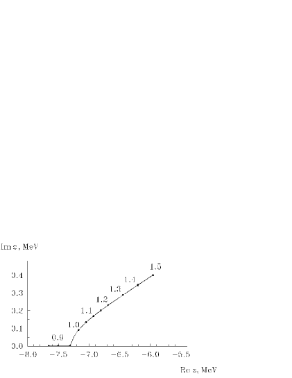
FIG. 3.: Trajectory of the resonance $z_{\rm res}(\mbox{3B})$ on the sheet $\Pi_{(0,1)}$ in the model system of three bosons with the nucleon masses. The potential $V^{G}(r)$ is used. Values of the barrier $V_{b}$ in MeV are given near the points marked on the curve.

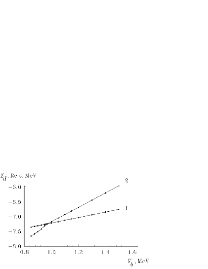
FIG. 4.: Dependence of the “deuteron” energy $E_{d}$ (curve 1) and real part of the resonance $z_{\rm res}(\mbox{3B})$ (curve 2) on the barrier value $V_{b}$.

Also, we have studied a model three–body system including identical spin-zero bosons with masses of the nucleon. Remind that the Faddeev integro-differential equations for such a three-boson system read exactly as the equations (4) except a necessity to replace the factor $-1/2$ in the expression (5) with unity. The boundary conditions for respective partial Faddeev components $U^{\rm 3B}_{L}(x,y)$ have the form (6) and (8) where instead of $a_{L}^{q}(z)$ and $A_{L}^{q}(\theta,z)$, one has to substitute $a_{L}^{\rm 3B}(z)$ and $A_{L}^{\rm 3B}(\theta,z)$.

Component of the truncated scattering matrix $S_{(0,1)}$ for the three-boson system is given in the state with the angular momentum $L$ by

$$s_{L}^{\rm 3B}(z)=1+2ia_{L}^{\rm 3B}(z).$$

Resonances on the sheet $\Pi_{(0,1)}$ in this state are roots of the equation $s_{L}^{\rm 3B}(z)=0$ considered on the physical sheet.

In the three-boson problem we restrict ourselves with a treating the s-state only and thereby, with a searching for zeros of the function $s_{L}^{\rm 3B}(z)$ at $L=0$. As a pairwise interaction between the bosons we have used the Gauss-type potential supplied with an additional Gauss repulsive barrier term,

$$V^{G}(r)=V_{0}\exp[-\mu_{0}r^{2}]+V_{b}\exp[-\mu_{b}(r-r_{b})^{2}]$$

where the values $V_{0}=-55$ MeV, $\mu_{0}=0.2$ fm^-2, $\mu_{b}=0.01$ fm^-2, $r_{b}=5$ fm have been fixed and the barrier amplitude $V_{b}$ varied. A resonance (with non-zero imaginary part) on the sheet $\Pi_{(0,1)}$ arises in the system concerned just due to the presence of the barrier term. Example of a surface of the $s_{0}^{\rm 3B}(z)$ absolute value for the barrier amplitude $V_{b}=1.5$ MeV is shown in Fig. 2 (for a $80\!\times\!80$ grid). A trajectory of the resonance $z_{\rm res}(\mbox{3B})$ (a zero of the function $s_{0}^{\rm 3B}(z)$) is shown for the changing barrier $V_{b}$ in Fig. 3. This trajectory was watched for the barrier $V_{b}$ decreasing in the interval between $1.5$ MeV and $0.85$ MeV. When drawing the trajectory, we have used a $160\!\times\!160$ grid. It can be seen from Fig. 3 that the behavior of the resonance $z_{\rm res}(\mbox{3B})$ is rather expected: with monotonously decreasing real part, the imaginary part of the resonance changes also monotonously.In Fig. 4 we plot both the trajectories of the resonance real part $\mathop{\rm Re}z_{\rm res}(\mbox{3B})$ and two-boson binding energy $E_{d}$. As one can see from this figure, the value of $|\mathop{\rm Re}z_{\rm res}(\mbox{3B})|$ increases more quickly than $|E_{d}|$, coinciding with $|E_{d}|$ at $V_{b}\cong 0.97$ MeV.

Trajectory of the resonance concerned in the lower complex half-plane is symmetric to the curve shown in Fig. 3 with respect to the real axis. Respective points, symmetric to those marked in Fig. 3, correspond to the same values of $V_{b}$. For $V_{b}\approx 0.95$ MeV the energy $z_{\rm res}(\mbox{3B})$ becomes real. In this point the resonances $z_{\rm res}(\mbox{3B})$ and $\overline{z}_{\rm res}(\mbox{3B})$ “collide” turning for $V_{b}<0.95$ MeV into a couple of virtual levels.