Neural Networks for Impact Parameter Determination

Abstract

An accurate impact parameter determination in a heavy ion collision is crucial for almost all further analysis. The capabilities of an artificial neural network are investigated to that respect. A novel input generation for the network is proposed, namely the transverse and longitudinal momentum distribution of all outgoing (or actually detectable) particles. The neural network approach yields an improvement in performance of a factor of two as compared to classical techniques. To achieve this improvement simple network architectures and a $5\times 5$ input grid in ($p_{t},p_{z}$) space are sufficient.

The physics of relativistic heavy ion collisions is motivated by the unique opportunity to study the properties of hot and dense nuclear matter [1, 2, 3, 4, 5, 6, 7, 8, 9].

For a detailed investigation of heavy ion collisions a proper event characterization is mandatory. In particular, the impact parameter, though not directly accessible experimentally, is among the most important characteristics for the description of the event geometry and selection.

For the investigation of highly compressed nuclear matter, it is important to select the most central collisions. On the other hand, recently discovered new phenomena such as pionic bounce–off and squeeze–out are only observed in semi-peripheral collisions.

There have been various proposals how to determine the impact parameter. Most of these are based on the mean particle multiplicity, the ratio of transverse to longitudinal energy deposition, a transverse momentum analysis (directivity-cut) or on a combination of these techniques. However, all previously mentioned methods have one thing in common: They tend to break down for very central collisions and are generally optimized for a certain impact parameter range. The achievable accuracy is estimated to be at best $\pm 1$ to $\pm 1.5$ fm.

Recently, neural networks have been suggested as tools for impact parameter determination [10, 11]. While offering an improvement of approximately 50 % as compared with “classical” techniques, their main shortcoming was the large amount of preprocessing neccessary for the selected input. Essentially, the proposed networks were used as multidimensional nonlinear fits to combine the (already known) impact-parameter dependence of the various input observables (a combination of three observables has been used) into a single function yielding the impact parameter.

The use of preprocessed input has the advantage of reducing the amount of input data (and therefore the computing time for the network output). It’s great disadvantage, however, is that only those correlations and informations preselected for the input can be accessed and optimized by the network. Previously unknown correlations between input observables and the desired output may be destroyed or left out through the preprocessing. Minimizing the amount of preprocessing allows for taking advantage of the full capabilities of the neural network. In addition, common preprocessing techniques are computationally expensive.

Those heavy ion collision events which are used as input for training and analyzing the network’s performance have to be supplied by a theoretical model rather than by experiment (otherwise it would be impossible to compare the network output with a target value for the impact parameter).

For the present study an extension of the Quantum Molecular Dynamics model (QMD) [12, 13, 14, 15] has been applied. It explicitly incorporates isospin and pion production via the delta resonance (IQMD) [16, 17, 18]. In the QMD model the nucleons are represented by Gaussian shaped density distributions, giving the nuclei a surface thickness of 1.5 fm. The initial momenta are randomly chosen between 0 and the local Thomas-Fermi-momentum. The $A_{P}$ projectile and $A_{T}$ target nucleons interact via two- and three-body Skyrme forces, a Yukawa potential, momentum dependent interactions, a symmetry potential (to achieve a correct distribution of protons and neutrons in the nucleus) and explicit Coulomb forces between the $Z_{P}$ and $Z_{T}$ protons. They are propagated according to Hamilton’s equations of motion. Hard N-N-collisions are included by employing the collision term of the well known VUU/BUU model [6, 19, 20, 21, 22]. The collisions are done stochastically, in a similar way as in the cascade models [23, 24]. In addition, the Pauli blocking (for the final state) is taken into account by regarding the phase space densities in the final states of a two-body collision. Clusters (e.g. deuterons and tritons) are formed via a configuration space coalescence model.

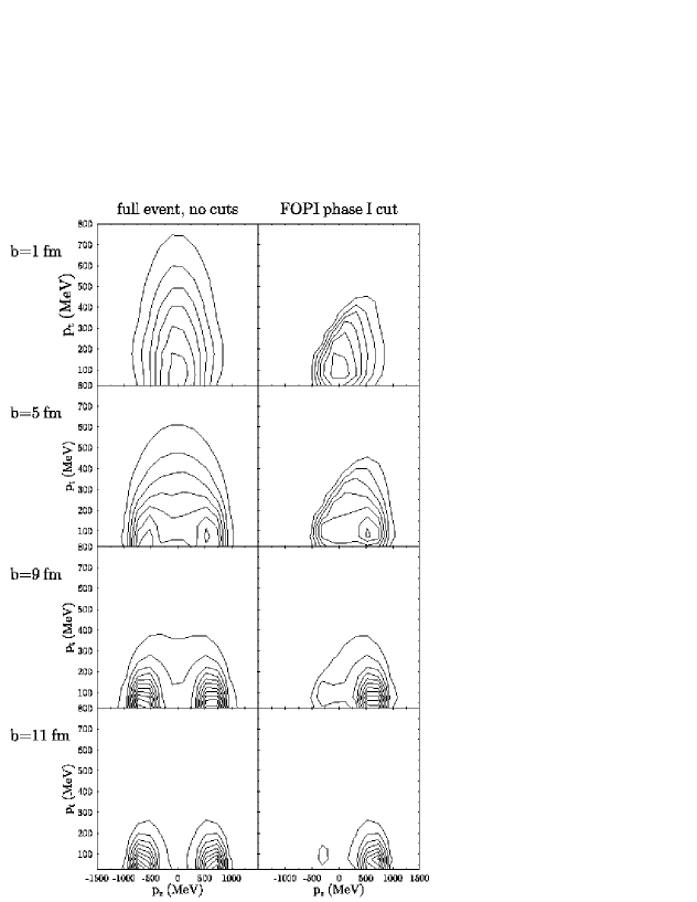
In order to minimize preprocessing and to allow the network to use “unknown correlations” the longitudinal and transverse momenta per nucleon of all baryons in the system were choosen as input. The left column of figure 1 shows the respective final state momentum distributions for impact parameters of 1, 5, 9 and 11 fm. In contrast to the full $4\pi$ information accessible via a QMD simulation, experiments usually have a limited acceptance. The right column of figure 1 shows the same momentum distributions as the left column, this time processed with the detector filter [26] of the FOPI experiment [25] at GSI. The filter does not only destroy the symmetry to the $p_{z}=0$ axis, but it also reduces drastically the available phase space information. The suggested neural algorithms should prove their usefulness both for the “ideal” $4\pi$ dataset and for the more “realistic” filtered set. A simplistic extrapolation of the network performance (from the “ideal” set to the “realistic” one), as performed for the preprocessed input of IMF-multipicity, $p_{x,dir}$ and ERAT in [11], is clearly not justified.

The event data have been transformed into a constant number of input components to be used with neural network. In this paper a new direct mapping of the momentum-state distribution to the network’s input is proposed. The momentum distributions is discretized in a two-dimensional grid. For each of the ($3\times 3$ to $20\times 20$, equally sized) momentum bins, the corresponding number of “hits” is calculated and used as one input component.

We now sketch the neural network algorithm used, a standard feed-forward two-layer perceptron trained by error-backpropagation [28, 29]. The network consists of a “hidden” layer of up to 20 nonlinear units receiving inputs from the applied data vector and transferring their signals to the output unit (a single linear output unit is used, whose continuous valued output represents the impact parameter).

Every (hidden or output) unit performs a weighted sum over all input signals. The hidden units calculate their own signals by applying a nonlinear “squashing” function $\sigma(x)$ to the result:

$$y_{j}^{\rm hid}=\sigma(x_{j}^{\rm hid})=\sigma\left(\sum_{k}w_{jk}^{\rm hid}\,y_{k}^{\rm in}\right)\quad.$$

As a squashing function $\sigma(x)=\tanh(x)$ is used. $y_{k}^{\rm in}$ is a component of the data vector. A connection weight (from input component $k$ to hidden unit $j$) is given by $w_{jk}^{\rm hid}$. The output unit is linear:

$$y^{\rm out}=\sum_{j}w_{j}^{\rm out}\,y_{j}^{\rm hid}\quad.$$

For each unit, a connection to a constant signal, $y_{0}\equiv 1$, is included which provides an activity threshold.

First, the network’s weights are initialized with small random values. For each learning pattern an output is produced during training. It is rated by the error function

$$E=\frac{\displaystyle 1}{\displaystyle 2}\left(\delta^{\rm out}\right)^{2}\;,$$

where

$$\delta^{\rm out}=y^{\rm target}-y^{\rm out}$$

with $y^{\rm target}$ as the desired output. Successively for each pattern, the weights are updated according to a gradient descent in the weight space with respect to the error function,

$$\Delta w_{l}^{\rm out}\;=\;-\varepsilon\,\frac{\displaystyle\partial E}{\displaystyle\partial w_{l}^{\rm out}}\;,\qquad\Delta w_{lm}^{\rm hid}\;=\;-\varepsilon\,\frac{\displaystyle\partial E}{\displaystyle\partial w_{lm}^{\rm hid}}\;,$$

with $\varepsilon>0$ as learning rate. This leads to the learning rules

$$\Delta w_{l}^{\rm out}=\varepsilon\,\delta^{\rm out}\,y_{l}^{\rm hid}$$

and

$$\Delta w_{lm}^{\rm h} = -\varepsilon\;\frac{\displaystyle\partial}{\displaystyle\partial w_{lm}^{\rm hid}}\left[\frac{\displaystyle 1}{\displaystyle 2}\left(y^{\rm target}-\sum_{j}w_{j}^{\rm out}\,y_{j}^{\rm hid}\right)^{2}\right]$$

$${\displaystyle\partial w_{lm}^{\rm h}}$$

$$= \varepsilon\,\delta^{\rm out}\,w_{l}^{\rm out}\,\sigma^{\prime}(x_{l}^{\rm hid})\,y_{m}^{\rm in}$$

$$= \varepsilon\,\delta_{l}^{\rm hid}\,y_{m}^{\rm in}\;,$$

where

$$\delta_{l}^{\rm hid}=\delta^{\rm out}\,w_{l}^{\rm out}\,\sigma^{\prime}(x_{l}^{\rm hid})\;.$$

The weight update values $\Delta w$ are added to the corresponding weights directly after each presentation of a learning sample (incremental learning).

The event data generated by the theoretical model were divided into three sets of equal size. The first set was used as training data, the second provided a criterion for stopping the learning process (in order to avoid overfitting), whereas the third one was used to determine the generalization ability of the system. Since there were virtually no limitations to the number of events available, large sets (1000 events each) could be used to reduce fluctuation of performance. For a complete learning session, typically several hundred cycles through the entire training data were necessary. Training was stopped when the performance on the criterion data set was best.

In contrast to the extensive training phase, very little calculation time is needed for the application of a trained network, so that it could be integrated into the data analysis process itself.

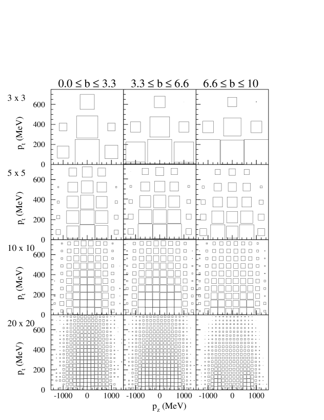
Figure 2 shows the effects of the chosen resolution (the number of input components) on the selected input for three impact parameter bins (central, medium and peripheral impact parameters). When increasing the resolution in order to improve the informational contents of the input the following points have to be taken into account:

• The computational time rises quadratically with the input grid dimension and therefore the processing time poses a constraint for the resolution.

• The increase in information through an increased resolution does not necessarily translate into an improved network performance (see figure 4).

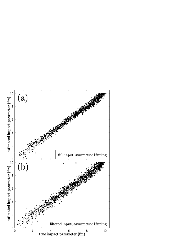
Sample results can be seen in figure 3. The true impact parameter is plotted versus the reconstructed impact parameter for full events (upper frame) and events processed with the filter of the FOPI experiment[26] (lower frame). Each dot represents one event. Both calculations have been performed with a $10\times 10$ input grid, 10 hidden units, and one output unit. In the lower frame the boundaries in $p_{t}$ and $p_{z}$ have been adapted to the acceptance range of the detector filter. In both cases the quality of reconstruction remains constant for the whole impact parameter range.

The effect of the detector filter can be seen in the slight broadening of the distribution. Although the symmetry along the $p_{z}=0$ axis has been broken and phase space severely reduced, the network at first glance seems to suffer only minor performance losses. A detailed quantitative analysis (see below) shows, however, that the network performance is diminished by $\approx 30$ % due to the detector filter. In view of the severe phase space limitations caused by the detector cut the network performance on the filtered sample is nevertheless remarkable.

Test calculations using three-dimensional ($p_{x},p_{y},p_{z}$) information as input rather than the reduced ($p_{t},p_{z}$) set, did not yield a significant performance improvement. On the contrary, the use of cartesian momenta is not feasible: For the proper definition of the $x$ and $y$ directions the reaction plane has to be determined. Experimentally this is a complicated task which can only be achieved within an uncertainty of approximately 30 degrees [31].

The performance of the network can be quantified by computing the average difference between the reconstructed and the true impact parameter:

$$\Delta b\;=\;\frac{\sum\limits_{i=1}^{N_{\rm events}}|b_{i}^{\rm true}-b_{i}^{\rm out}|}{N_{\rm events}}$$

In the first test case ($10\times 10$ input grid, 10 hidden units) the network achieved $\Delta~{}b~{}=~{}0.25$ fm for the unfiltered and $\Delta~{}b~{}=~{}0.35$ fm for the filtered input.

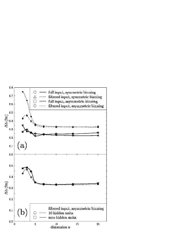
How does the performance vary with the dimension of the input grid and the number of hidden units? In figure 4a) the performance $\Delta b$ is plotted versus the input grid dimension (the square root of the number of input components) for the unfiltered and filtered data with and without adaption of the input boundaries to the available phase space. In the region of optimum network performance this adaption has little effect; only for very small input grid dimensions is a large effect (a performance gain by 40%) obtained.

Far more important is the input grid dimension itself. In the limit of a ($2\times 2$) input grid one reduces the input basically to the ratio of transverse to longitudinal degrees of freedom. This corresponds to the well known directivity criterion for impact parameter selection. Increasing the input grid dimension from 2 to 5 improves the performance by a factor of up to two. This indicates that there are correlations present in the ($p_{z},p_{t}$) distribution of the event, which are sensitive to the impact parameter and are not covered by the directivity observable or any other related ratio of transverse to longitudinal degrees of freedom. However, no significant performance gain is obtained when increasing the input grid dimension beyond 10. This finding is important, since it shows that a further increase in information presented to the network (via a larger input grid) does not lead to a better reconstructive power for the impact parameter. Therefore one can conclude that all ($p_{z},p_{t}$) correlations useful for the impact parameter reconstruction can be contained in a $5\times 5$ grid of equidistant bins covering the relevant (detectable) momentum space area. The performance loss due to the detector filter remains constant for dimensions larger than 4 and increases for those smaller than 4.

In figure 4b) the performance $\Delta b$ is again plotted versus the input grid dimension. Filtered input with asymmetric binning was used. Two calculations are shown, one with 10 hidden units and one without any hidden units, where the input components were connected directly to the output unit (also called simple perceptron). In the latter case the learning rule becomes particularly simple, as the input components replace the hidden units.

For input grid dimensions larger than 5, the number of hidden units seems to be totally irrelevant, so that the simple perceptron suffices. In essence the task for the network appears to be a linear one. This simple network configuration has the great advantage that one can study its working mechanisms in great detail: The reconstructed impact parameter is obtained essentially by computing the scalar product between the input vector (a one-dimensional representation of the $10\times 10$ input grid) and a weight vector. An “optimal” set of weights minimizing the average error for all events of the training set could in fact be determined via calculation and inversion of a Hessian matrix. A numerical test confirmed this. For nonlinear systems with hidden units, however, grossly deteriorated generalization capabilities would be expected. For better comparability, the learning process was therefore used in all cases.

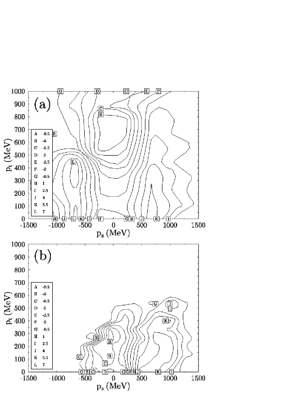
In figure 5 the weight vector of a ($10\times 10$) network without hidden units is mapped onto the representation of the input grid as displayed in figure 2, third row. Frame a) shows the distribution for unfiltered input, whereas frame b) shows the distribution for the filtered input. The distribution of weights correlates directly to the presented physical input. Areas in the ($p_{z},p_{t}$) plane associated with small impact parameters are assigned negative weights (contour lines A-G), whereas those associated with large impact parameters carry positive weights (contour lines H-L). This specific distribution becomes intuitively clear if one remembers that the scalar product of input vector and weight vector is simply the sum of the number of hits in each momentum bin multiplied by their corresponding weights. Since the result of this sum is the reconstructed impact parameter, hits in peripheral areas must contribute large positive values whereas hits in central areas must compensate with negative values.

For the application of the proposed technique on experimental data the neural network needs to be trained on a data-set with known impact parameters, i.e. a data-set generated by a transport model. This model must be able to accurately reproduce the final state of the heavy ion collision, most importantly the particle and fragment multiplicities and the respective double differential cross sections in ($p_{t},p_{z}$) space. This procedure, however, creates a model bias. It’s magnitude can be estimated by generating two sets of weights from two different transport models. Then the network can be applied with both sets on the same experimental data and the difference in the reconstructed impact parmeters yields an estimate on the model bias involved.

In summary, we have applied neural network techniques to the problem of impact parameter determination in relativistic heavy ion collisions. As input the transverse and longitudinal momentum distributions of all outgoing (or detectable) particles were discretized in two-dimensional grids of varying size. The neural network approach yields an improvement of a factor of two as compared with classical techniques. All information necessary to achieve this improvement is present in a $5\times 5$ grid in ($p_{t},p_{z}$) space. Simple network algorithms suffice, hidden units are not necessary.

FIG. 1.: $\frac{dN}{p_{t}dp_{t}dp_{z}}$ (all momenta per nucleon) for nucleons and fragments in Au+Au collisions at 1 GeV/nucleon and in the final state, i.e. after all collisions have ceased. The left column shows the full $4\pi$ acceptance whereas the right column shows the events filtered with the acceptance of the FOPI detector (phase I). The different rows depict different impact parameter bins.

FIG. 2.: Discretization of $\frac{dN}{p_{t}dp_{t}dp_{z}}$ for input into the neural network. The columns refer to central, medium and peripheral collisions (left to right). The rows show the input for different grid dimensions (top to bottom: 3, 5, 10 and 20). The area of the squares is proportional to the number of particles in the bins.

FIG. 3.: True impact parameter versus the reconstructed impact parameter for full events (upper frame) and events processed with the filter of the FOPI experiment (lower frame). Each dot represents one event.

FIG. 4.: Network performance $\Delta b$ versus input grid dimension $n$. The upper frame compares calculations with and without detector filter. The original boundaries which cover the available phase space information in the unfiltered case are marked as symmetric binning whereas the boundaries adapted to the detector acceptance of the filtered data-set are marked as asymmetric binning. In the lower frame calculations with and without hidden units are displayed.

FIG. 5.: Weight vector mapped onto the representation of the input grid for unfiltered (top) and filtered (bottom) input. The weight distribution is directly correlated to the physical content of the input.

REFERENCES

- [1] W. Scheid, R. Ligensa and W. Greiner. Phys. Rev. Lett. 21, 1479 (1968).
- [2] W. Scheid, H. Müller and W. Greiner. Phys. Rev. Lett. 32, 741 (1974).
- [3] J. Maruhn and W. Greiner. In A. D. Bromley, editor, Treatise on Heavy Ion Science, Vol. 4,Plenum Press, New York and London, 1985, p. 565.
- [4] L. P. Csernai and J. I. Kapusta. Phys. Reports 131, 225 (1986).
- [5] R. Stock. Phys. Reports 135, 261 (1986).
- [6] H. Stöcker and W. Greiner. Phys. Reports 137, 277 (1986).
- [7] R. B. Clare and D. Strottman. Phys. Reports 141, 179 (1986).
- [8] B. Schürmann, W. Zwermann and R. Malfliet. Phys. Reports 147, 3 (1986).
- [9] W. Cassing, V. Metag, U. Mosel and K. Niita. Phys. Reports 188, 365 (1990).
- [10] S. A. Bass, A. Bischoff, C. Hartnack, J. A. Maruhn, J. Reinhardt, H. Stöcker and W. Greiner. J. Phys. G20, L21 (1994).
- [11] C. David, M. Freslier, J. Aichelin. Phys. Rev.C51, 1453 (1995).
- [12] J. Aichelin and H. Stöcker. Phys. Lett. B176, 14 (1986).
- [13] J. Aichelin, A. Rosenhauer, G. Peilert, H. Stöcker, and W. Greiner. Phys. Rev. Lett. 58, 1926 (1987).
- [14] J. Aichelin. Phys. Reports 202, 233 (1991).
- [15] S. A. Bass, C. Hartnack, H. Stöcker, and W. Greiner. Phys. Rev. C51, 3343 (1995).
- [16] Ch. Hartnack, H. Stöcker, and W. Greiner. In H. Feldmeier, editor, Proc. of the International Workshop on Gross Properties of Nuclei and Nuclear Excitation, XVI, Hirschegg, Kleinwalsertal, Austria (1988).
- [17] C. Hartnack, L. Zhuxia, L. Neise, G. Peilert, A. Rosenhauer, H. Sorge, J. Aichelin, H. Stöcker, and W. Greiner. Nucl. Phys. A495, 303 (1989).
- [18] Ch. Hartnack. PhD thesis, GSI-Report 93-5 (1993).
- [19] H. Kruse, B. V. Jacak, and H. Stöcker. Phys. Rev. Lett. 54, 289 (1985).
- [20] J. Aichelin and G. Bertsch. Phys. Rev. C31, 1730 (1985).
- [21] G. Wolf, G. Batko, W. Cassing, U. Mosel, K. Niita, and M. Schäfer. Nucl. Phys. A517, 615 (1990).
- [22] B. A. Li, W. Bauer, and G. F. Bertsch. Phys. Rev. C44, 2095 (1991).
- [23] Y. Yariv and Z. Frankel. Phys. Rev. C20, 2227 (1979).
- [24] J. Cugnon. Phys. Rev. C22, 1885 (1980).
-
[25]
S. C. Jeong and the FOPI collaboration.
Phys. Rev. Lett. 72, 3468 (1994).
A. Gobbi and the FOPI collaboration. Nucl. Instrum. Meth. A324, 156 (1993). - [26] S. Hölbling and the FOPI collaboration. Taken from the reference library FLIB of the FOPI collaboration.
- [27] Y.I. Grigorian for the FOPI-Collaboration. GSI Scientific Report 1991 (1992), 28, and various other contributions by the FOPI-Collaboration in the same report.
- [28] J.L. McClelland, D.E. Rumelhart (eds.): Parallel Distributed Processing, 2 vols., MIT Press, Cambridge (1986).
- [29] see also B. Müller and J. Reinhardt, Neural Networks, Springer-Verlag, 1990, and references therein
- [30] P. Danielewicz and G. Odyniec. Phys. Lett. B157, (1985), 146.
- [31] H. Gutbrod, A. M. Poskanzer and H. G. Ritter. Rept. Prog. Phys. 52, (1989), 1267.