The nucleon spectral function at finite temperature and the onset of superfluidity in nuclear matter

Abstract

Nucleon selfenergies and spectral functions are calculated at the saturation density of symmetric nuclear matter at finite temperatures. In particular, the behaviour of these quantities at temperatures above and close to the critical temperature for the superfluid phase transition in nuclear matter is discussed. It is shown how the singularity in the thermodynamic T-matrix at the critical temperature for superfluidity (Thouless criterion) reflects in the selfenergy and correspondingly in the spectral function. The real part of the on-shell selfenergy (optical potential) shows an anomalous behaviour for momenta near the Fermi momentum and temperatures close to the critical temperature related to the pairing singularity in the imaginary part. For comparison the selfenergy derived from the K-matrix of Brueckner theory is also calculated. It is found, that there is no pairing singularity in the imaginary part of the selfenergy in this case, which is due to the neglect of hole-hole scattering in the K-matrix. From the selfenergy the spectral function and the occupation numbers for finite temperatures are calculated.

(MPG-VT-UR 65/95, submitted to Phys. Rev. C)

I Introduction

Heavy ion reactions at intermediate energies probe the nuclear equation of state in a broad temperature and density range. One tries to extract from the observables signals for cluster formation, multifragmentation or the liquid-gas phase transition. The theoretical description of such phenomena demands to go beyond the usual quasiparticle description for the equilibrium properties (equation of state) as well as for the non-equilibrium properties (BUU-simulations). The need to go beyond the quasiparticle approximation in the description of nuclear matter is further advocated by the electron scattering experiments from heavy nuclei. These experiments give a clear evidence that the one-nucleon spectral function shows pronounced deviations from mean field estimates, which are due to NN-correlations [1]. The effect of these correlations can most accurately be studied for nuclear matter [2].

A systematic quantum statistical approach for the description of dense nuclear matter can be given using Green function theory. For the description of phenomena like the formation of clusters (bound states) in the medium or the onset of a superfluid phase one has to allow for a finite lifetime (damping) of the one particle states. Such a treatment can be based on the nucleon spectral function, which is defined in terms of the real and imaginary parts of the selfenergy. Having the nucleon spectral function at the disposal, one is able to determine the momentum distribution, the response function as well as the nuclear equation of state including correlations beyond the mean field level.

Most of the existing calculations of the nucleon spectral function have been done for zero temperature nuclear matter at the saturation density $n_{0}$. In refs. [3, 4, 5] it is shown that the quasiparticle description is only valid near the Fermi energy. In general, the spectral function has a considerable width indicating that the one-particle states are strongly damped at the saturation density. Baldo et al. [3] calculated the on- and off-shell properties of the nucleon mass operator and the nucleon spectral function. They stressed the importance to retain the full frequency dependence of the selfenergy for the calculation of the spectral function. Köhler [4] compared the nucleon spectral function calculated within Green function theory with a calculation done in Brueckner theory. He pointed out the near equivalence between the two theories at zero temperature. Vonderfecht et al. [5] used Green function theory to calculate the nucleon selfenergy within the ladder approximation at zero temperature. They emphasized the need to correctly treat the pairing correlations contained in this approximation if hole-hole propagation is included in the kernel of the vertex function (thermodynamic T-matrix). Benhar et al. [6] calculated spectral functions for nuclear matter using the hyper-netted chain (HNC) method. The spectral function and the nucleon momentum distribution in nuclear matter were calculated by Benhar et al. [7] at densities below the saturation density within orthogonal correlated basis functions theory (OCBF). As a result, they find that with decreasing density the discontinuity at the Fermi surface decreases. This means that the momentum distribution does not approach the non-interacting response with decreasing density. This was interpreted as being due to the attraction in the N-N interaction leading to the formation of “bound pairs” of nucleons. Van Neck et al. [8] use correlated basis functions theory (CBF) with the Urbana $v_{14}$ interaction to calculate the nuclear matter spectral function and momentum distribution below $n_{0}$. In agreement with the previous authors they found that the momentum distribution does not reach the non-interacting one with decreasing density. De Jong et al. [9] calculated the nucleon spectral function based on an extension of the relativistic Dirac-Brueckner scheme.

First finite temperature calculations of the nucleon self energy were carried out by Grangé et al. [10], Röpke et al. [11] (in connection with the e.o.s.) and Köhler [12]. The latter author found a pronounced temperature dependence of the spectral function at the saturation density. Using the extended quasiparticle approximation for the nucleon spectral function Schmidt et al. [13] included the formation of two-nucleon correlations (in particular bound states) in the equation of state of nuclear matter. The finite temperature nucleon spectral function in the low-density region of nuclear matter was calculated by Alm et al. [14] demonstrating the necessity to include the contribution of two-nucleon bound states to the one-nucleon spectral function at low density. These authors find that genuine bound state formation in nuclear matter is only possible at extremely low densities ($n\leq 0.05\,n_{0}$, $T=10\;{\rm MeV}$). With increasing density the bound states are dissolved in the medium (Mott effect). However, the formation of two-nucleon pairs in the continuum as well as their possible Bose condensation [15] can take place at these higher densities as well. The necessity to include the deuteron singularity in the two-particle T-matrix into the description of nucleon-nucleus scattering a low energies within the folding model was demonstrated by Love et al. [16].

Within this paper we would like to discuss the nucleon selfenergy, spectral function and momentum distribution at the saturation density and at finite temperatures. In particular, we will concentrate on low temperatures near the critical temperature for the superfluid phase transition in symmetric nuclear matter, which has a maximum of $\sim 5-6\;{\rm MeV}$ at densities below $n_{0}$ [15]. This phase transition has recently been discussed by some authors in particular with respect to the possible formation of a condensate of neutron-proton-pairs in the ${}^{3}{\rm S}_{1}-{}^{3}{\rm D}_{1}$-channel [17] and the relation to the Bose condensation of deuterons in low-density nuclear matter [18]. Moreover, Baldo et al. [19] suggest that this could be a possible mechanism of deuteron formation in heavy-ion reactions at intermediate energy. The onset of the superfluid phase is contained in the thermodynamic T-matrix in the ladder approximation [15]. It manifests itself as a pole defining the critical temperature for the thermodynamic T-matrix [20]. It could be shown that already above the critical temperature the T-matrix shows a resonance-like behaviour which could be understood as a precursor effect of the superfluid phase transition [21]. Consequently, near the critical temperature the selfenergy and correspondingly the spectral function should reflect this resonance-like behaviour of the T-matrix. In this paper we will demonstrate how the T-matrix, the nucleon selfenergy and spectral function are changed when approaching the critical temperature for the superfluid phase transition from above.

In chapter II we derive a set of selfconsistent expressions for the retarded nucleon selfenergy and the nucleon spectral function at finite temperature within the framework of Matsubara Green functions. In the following chapter III the differences to the usual Brueckner theory generalized to finite temperatures are pointed out. The chapter IV contains results for the T-matrix and the K-matrix and the corresponding selfenergies including the optical potential at finite $T$. Within chapter V the corresponding spectral functions and occupation numbers are presented.

II Green Function Formalism and Approximations

For the derivation of the selfenergy and the spectral function we use the Matsubara Green function technique as outlined in ref. [22]. We put $\hbar,k_{B}=1$ throughout the paper. From the definition of the one-particle spectral function $A(1,\omega)=i[G(1,\omega+i0)-G(1,\omega-i0)]$ and from the retarded selfenergy $\Sigma$ the spectral function according to the Dyson equation reads

$$A(1,\omega)=\frac{2\,{\rm Im}\,\Sigma(1,\omega)}{[\omega-\frac{p_{1}^{2}}{2m}-{\rm Re}\,\Sigma(1,\omega)]^{2}+[{\rm Im}\,\Sigma(1,\omega)]^{2}}\mbox{ ,}$$ (1)

where $1=\{p_{1},\sigma_{1},\tau_{1}\}$ denotes momentum, spin and isospin of a single particle.
The one-particle spectral function (1) fulfills the sum rule

$$\int\frac{{\rm d}\omega}{2\pi}A(1,\omega)=1\mbox{ .}$$ (2)

It determines the macroscopic properties of the system such as the occupation $n_{1}$ of single particle states given by

$$n_{1}(\mu,T)=\int\frac{{\rm d}\omega}{2\pi}f(\omega)A(1,\omega)\mbox{ ,}$$ (3)

where $f(\omega)=\{\exp((\omega-\mu)/T)+1\}^{-1}$ is the Fermi distribution. The equation of state of nuclear matter, where the nucleon density $n$ is a function of the chemical potential $\mu$ and the temperature $T$, reads

$$n(\mu,T)=\frac{1}{\Omega}\sum_{1}n_{1}(\mu,T)\mbox{ ,}$$ (4)

with $\Omega$ being the normalization volume.

For the evaluation of the selfenergy $\Sigma$ in eq. (1) approximations have to be made. We start from a cluster decomposition of the selfenergy [23], which is given by the following set of diagrams

   ,

(5)

where $z_{\nu}$ is the Fermionic Matsubara frequency. The cluster decomposition is appropriate for the consideration of $n$-particle correlations via the $n$-particle T-matrix $T_{n}$. Within this paper we restrict to $n=2$, i.e. to two-particle correlations represented by the first diagram in eq. (5). Within the ladder approximation the two-particle T-matrix is given by

$$T(121^{\prime}2^{\prime},z)=V(121^{\prime}2^{\prime})+\frac{1}{\Omega}\sum_{3,4,5,6}V(1234)\,G_{2}(3456,z)\,T(561^{\prime}2^{\prime},z)\mbox{ ,}$$ (6)

where the quantity $G_{2}$ is defined as the product of two full one-particle Green functions given in spectral representation as

$$G_{2}(121^{\prime}2^{\prime},z)=\int\frac{{\rm d}\omega}{2\pi}\int\frac{{\rm d}\omega^{\prime}}{2\pi}\frac{1-f(\omega)-f(\omega^{\prime})}{\omega+\omega^{\prime}-z}A(1,\omega)A(2,\omega^{\prime})\delta_{11^{\prime}}\delta_{22^{\prime}}\mbox{ .}$$ (7)

Using the spectral representation for the one particle Green function as well as for the T-matrix [23] the first diagram in (5) yields

$$\Sigma(1,\omega+i0)=\frac{1}{\Omega}\sum_{2}\int\frac{{\rm d}\omega^{\prime}}{2\pi}A(2,\omega^{\prime})\left(f(\omega^{\prime})V_{\rm ex}(1212)-\int\frac{{\rm d}E}{\pi}\frac{[f(\omega^{\prime})+g(E)]{\rm Im}T_{\rm ex}(1212,E)}{E-\omega^{\prime}-\omega-i0}\right)\mbox{ ,}$$ (8)

where $f(\omega)$ is the Fermi distribution and $g(E)=\{\exp((E-2\mu)/T)-1\}^{-1}$ the Bose distribution function for the two-nucleon states. $T_{\rm ex}$ and $V_{\rm ex}$ denote matrix elements of the retarded T-matrix and of the potential including exchange.

The ladder T-matrix equation (6,7) as well as the selfenergy (8) contain the one-particle spectral function (1) and thus form a selfconsistent set of equations. A solution of the complicated set of equations (1), (6,7) and (8) can be achieved by iteration. In the first step of iteration we replace the spectral function in eq. (8) by a quasiparticle spectral function

$$A^{\rm QP}(1,\omega)=2\pi\delta(\omega-\epsilon_{1})\mbox{ ,}$$ (9)

where the quasiparticle energy $\epsilon_{1}$ is defined as

$$\epsilon_{1}=\frac{p_{1}^{2}}{2m}+{\rm Re}\,\Sigma(1,\omega)\mid_{\omega=\epsilon_{1}}\mbox{ .}$$ (10)

Inserting the quasiparticle spectral function (9) in eq. (7) results in the quasiparticle approximation for the two-particle T-matrix (6). Within these approximations the following expressions for the imaginary and real part of the selfenergy (8) are obtained

$${\rm Im}\,\Sigma(1,\omega)=\frac{1}{\Omega}\sum_{2}[f(\epsilon_{2})+g(\epsilon_{2}+\omega)]\>{\rm Im}T_{\rm ex}(1212,\epsilon_{2}+\omega)$$ (11)

and

$${\rm Re}\,\Sigma(1,\omega)=\frac{1}{\Omega}\sum_{2}\left(f(\epsilon_{2}){\rm Re}T_{\rm ex}(1212,\epsilon_{2}+\omega)-{\bf P}\int\frac{{\rm d}E}{\pi}\frac{g(E){\rm Im}T_{\rm ex}(1212,E)}{E-\epsilon_{2}-\omega}\right)\mbox{ ,}$$ (12)

where P denotes the Cauchy principal value. $T_{\rm ex}$ ist calculated in the quasiparticle approximation. Rather then (12) we use in the numerical calculation the real part from the dispersion relation (Kramers-Kronig-relation) in the form

$${\rm Re}\,\Sigma(1,\omega)=\Sigma^{\rm HF}(1)+{\bf P}\int\frac{d\omega^{\prime}}{\pi}\frac{{\rm Im}\,\Sigma(1,\omega^{\prime})}{\omega-\omega^{\prime}}\mbox{ ,}$$ (13)

where $\Sigma^{\rm HF}(1)$ denotes the Hartree-Fock shift. This was numerically checked to be equivalent with the explicit formula (12).

The bare nucleon-nucleon interaction was approximated by a separable ansatz

$$V_{\alpha}^{LL^{\prime}}(p,p^{\prime})=\sum_{i,j=1}^{\rm rank}w_{\alpha i}^{L}(p)\lambda_{\alpha ij}w_{\alpha j}^{L^{\prime}}(p^{\prime})\mbox{ .}$$ (14)

The T-matrix then can be given algebraically as

$$T^{LL^{\prime}}_{\alpha}(p,p^{\prime},P,E)=\sum_{ijk}w_{\alpha i}^{L}(p)[1-J_{\alpha}(P,E)]_{ij}^{-1}\lambda_{\alpha jk}w^{L^{\prime}}_{\alpha k}(p^{\prime})\mbox{ ,}$$ (15)

$$J_{\alpha}(P,E)_{ij}=\int\frac{{\rm d}^{3}{\bf p}}{(2\pi)^{3}}\sum_{nL}w_{\alpha n}^{L}\lambda_{\alpha in}w_{\alpha j}^{L}(p)\frac{<1-f({\bf P}/2+{\bf p})-f({\bf P}/2-{\bf p})>}{E-\epsilon(P/2+p)-\epsilon(P/2-p)}\mbox{ ,}$$ (16)

where $<...>$ denotes the usual angle averaging in the Pauli operator. Having the selfenergy at our disposal the spectral function follows from equation (1). The quasiparticle energies $\epsilon_{1}$ as defined by (10) were determined in Hartree-Fock approximation

$$\Sigma^{\rm HF}(1)=\frac{1}{\Omega}\sum_{2}f(\epsilon_{2})V_{\rm ex}(1,2,1,2)\mbox{ .}$$ (17)

With the T-matrix (15) one is able to calculate the critical temperature for superfluidity using the Thouless-criterion [20]. It has been demonstrated in ref. [20] that this coincides with the critical temperature found in BCS-theory. For the separable ansatz (14) it reads

$$\det[1-J_{\alpha}(P=0,E=2\mu,T=T_{c})]_{ij}=0\mbox{ .}$$ (18)

The Thouless-criterion for nuclear matter has already been evaluated in ref. [15].

III Selfenergy in Brueckner theory

Brueckner theory is only applicable to zero temperature systems. The near equivalence to Green function results has been demonstrated in this case as already pointed out above. A $T>0$ extension of Brueckner theory was formulated by Bloch and De Dominicis [24]. An obvious difference between the two approaches (Brueckner and Green function) is that the former only includes particle ladders while the latter also includes hole ladders in defining the effective interaction. It is of some interest to numerically study the effect of this difference. We therefore define a Brueckner K-matrix as in eq. (6) with T replaced by K. The propagator (7) is however modified by the replacement

$$1-f(\omega)-f(\omega^{\prime})\longrightarrow(1-f(\omega))(1-f(\omega^{\prime}))\mbox{ .}$$ (19)

The selfenergy ($V_{\rm B}$) in Brueckner theory is given by [25]

$$V_{\rm B}(1,\omega) = \frac{1}{\Omega}\sum_{2}\Big{(}f(\epsilon_{2})K_{\rm ex}(1212,\epsilon_{2}+\omega)$$ (21)

$$+{}\frac{1}{\Omega}\sum_{3,4}{|K_{\rm ex}(1234,\epsilon_{3}+\epsilon_{4})|}^{2}\frac{[1-f(\epsilon_{2})]f(\epsilon_{3})f(\epsilon_{4})}{\omega+\epsilon_{2}-\epsilon_{3}-\epsilon_{4}-i\eta}\delta_{{\bf p}_{1}+{\bf p}_{2},{\bf p}_{3}+{\bf p}_{4}}\Big{)}\mbox{ .}$$

For the discussion below, let us denote the two terms in eq. (21) by $V_{\rm B}^{1}$ and $V_{\rm B}^{2}$. The second term, $V_{\rm B}^{2}$, is often referred to as the Brueckner second order rearrangement potential. At a temperature $T=0$ it is zero for states above the Fermi-surface and negative for states below, while the first term is positive for states above and zero below the Fermi-surface. As explained below, the retarded selfenergy in (finite-temperature) Brueckner theory, denoted by $\Sigma_{\rm B}$, is given by

$${\rm Im}\,\Sigma_{\rm B}(1,\omega)={\rm Im}\,V_{\rm B}^{1}(1,\omega)-{\rm Im}\,V_{\rm B}^{2}(1,\omega)\mbox{ ,}$$ (22)

$${\rm Re}\,\Sigma_{\rm B}(1,\omega)={\rm Re}\,V_{\rm B}(1,\omega)={\rm Re}\,V_{\rm B}^{1}(1,\omega)-{\bf P}\int\frac{d\omega^{\prime}}{\pi}\frac{{\rm Im}\,V_{\rm B}^{2}(1,\omega^{\prime})}{\omega-\omega^{\prime}}\mbox{ .}$$ (23)

This quantity is to be compared to the Green function $\Sigma$ defined in the previous section.

While $\Sigma_{\rm B}$ is calculated numerically according to eqs. (21), (22), and (23), rewriting these expressions to parallel those in the last section would facilitate comparisons between the two formalisms. To this end, one can, invoking unitarity on the imaginary part of the second term of eq. (21), write ${\rm Im}\,V_{\rm B}$ as [25]

$${\rm Im}\,V_{\rm B}(1,\omega)=\frac{1}{\Omega}\sum_{2}[f(\epsilon_{2})-\bar{g}(\epsilon_{2},\omega)]{\rm Im}\,K_{\rm ex}(1212,\epsilon_{2}+\omega)\mbox{ ,}$$ (24)

with

$$\bar{g}(\epsilon_{2},\omega)=\frac{[1-f(\epsilon_{2})]g(\epsilon_{2}+\omega)}{g(\epsilon_{2}+\omega)+1}=f(\epsilon_{2})e^{-\beta(\omega-\mu)}\mbox{ .}$$ (25)

Notice that at $2\mu=\epsilon_{2}+\omega$ where $g$ has a singularity $\bar{g}$ is finite. It was argued in ref. [27] that the Brueckner $V_{\rm B}$ should be identified with the chronological potential $\Sigma^{\rm c}$ which is related to $\Sigma$ [26, 27] by

$${\rm Im}\,\Sigma^{\rm c}(1,\omega)=\tanh(\frac{1}{2}\beta(\omega-\mu))\,{\rm Im}\,\Sigma(1,\omega)\mbox{ .}$$ (26)

In our notations here, this says, for $T>0$, one can obtain ${\rm Im}\,\Sigma_{\rm B}$ from

$${\rm Im}\,\Sigma_{\rm B}=\frac{{\rm Im}\,V_{\rm B}}{\tanh(\frac{1}{2}\beta(\omega-\mu))}\mbox{ .}$$ (27)

Now eqs. (24) and (25) also give a simple relation between the two terms contributing to ${\rm Im}\,V_{\rm B}(1,\omega)$:

$${\rm Im}\,V_{\rm B}^{2}(1,\omega)=-e^{-\beta(\omega-\mu)}{\rm Im}\,V_{\rm B}^{1}(1,\omega)\mbox{ .}$$ (28)

It is then obvious that the division by the tanh function, in obtaining ${\rm Im}\,\Sigma_{\rm B}$ from ${\rm Im}\,V_{\rm B}$, is equivalent to just switching the sign of ${\rm Im}\,V_{\rm B}^{2}(1,\omega)$:

$${\rm Im}\,\Sigma_{\rm B}(1,\omega)=(1+e^{-\beta(\omega-\mu)}){\rm Im}\,V_{\rm B}^{1}(1,\omega)\mbox{ ,}$$ (29)

as stated in eq. (22) above.

An equivalent way of expressing the foregoing correspondence between ${\rm Im}\,V_{\rm B}(1,\omega)$ and Green function quantities is identifying $2i\,{\rm Im}\,V_{\rm B}^{1}$ and $2i\,{\rm Im}\,V_{\rm B}^{2}$ with, respectively, $\Sigma^{<}$ and $\Sigma^{>}$, the nonequilibrium extensions of which govern the loss and gain collision terms in a transport equation [28]. The on-shell version of this correspondence was pointed out by Cugnon et al [29].

IV Results for the T-matrix (K-matrix) and the nucleon selfenergy

In this exploratory calculation we used a rank one separable approximation (Yamaguchi potential [30]) as well as a rank two parametrization of Mongan [31]. The formfactors of the barely attractive Yamaguchi potential are of the following form

$$w_{\alpha}(p)=\frac{\lambda_{\alpha}}{p^{2}+\gamma^{2}}\mbox{ ,}$$ (30)

where the coupling constant and the effective range are given by

$$\lambda_{\alpha} = \left\{\begin{array}[]{rl}12.3178\;({\rm MeV}\,{\rm fm}^{-1})^{\frac{1}{2}}&\alpha={}^{1}{\rm S}_{0}\\ 14.6988\;({\rm MeV}\,{\rm fm}^{-1})^{\frac{1}{2}}&\alpha={}^{3}{\rm S}_{1}\end{array}\right.\mbox{ ,}$$ (33)

$$\gamma = 1.4488\;{\rm fm}^{-1}\mbox{ .}$$ (34)

The formfactors for the rank two Mongan potential, which contains in addition to a long-range attractive a short-range repulsive term, have the same form as given in eq. (30). The corresponding parametrization is given in ref. [31]. For numerical convenience we restricted only to S-waves (${}^{1}{\rm S}_{0},{}^{3}{\rm S}_{1}$) which give the dominant contribution to the T-matrix at low energies.

As we are concerned within this paper with the modification of the selfenergy near the critical temperature for the superfluid phase transition in symmetric nuclear matter, we first study the onset of superfluidity in the temperature-density plane of nuclear matter. In Fig. 1 the critical temperature for superfluidity (18) ($\alpha={}^{3}{\rm S}_{1}$) is given as a function of the density. The solid curve refers to the Yamaguchi potential whereas the dashed curve is for the Mongan interaction.

FIG. 1.: The critical temperature for superfluidity in symmetric nuclear matter (${}^{3}{\rm S}_{1}$-channel) according to eq. (18) as a function of density for the Yamaguchi and the Mongan potential. The saturation density $n_{0}$ is indicated.

Due to the repulsive component present in the Mongan interaction the critical temperature is reduced compared to the barely attractive Yamaguchi potential. These curves are in qualitative agreement with the calculations done in ref. [15]. In the following calculations we fix the density to $n=n_{0}$ (dotted line in Fig. 1 and vary the temperature.

The key quantity for the calculation of the selfenergy within the ladder-approximation is the thermodynamic T-matrix. In Fig. 2 the imaginary and the real part of the diagonal matrix elements of the thermodynamic T-matrix (triplett-channel) of the Green function theory (15) are given as a function of the energy argument at fixed relative momentum $p$ and total momentum $P=0$ as well as at a fixed chemical potential $\mu$. The imaginary part shows a zero, which is located at $\omega=2\mu$ independent on the temperature. This is due to the fact that the imaginary part of the T-matrix (15,16) is proportional to

$$1-2f(\epsilon(p))=g^{-1}(2\epsilon(p))f(\epsilon(p))f(\epsilon(p))\mbox{ ,}$$ (35)

which is obviously zero at $2\epsilon(p)=2\mu$ for any temperature. With decreasing temperature the slope of the imaginary part of the T-matrix at $\omega=2\mu$ increases; at temperatures near $T_{c}$ ($T_{c}=4.02\;{\rm MeV}$ in our case) it has a characteristic principal value structure. The real part develops the corresponding peak at $\omega=2\mu$ while approaching the critical temperature from above. Finally at $T=T_{c}$ the real part of the T-matrix diverges in accordance with the Thouless criterion [20].

The results of Fig. 2 can be compared with the $T=0$ results by Ramos et al. [32]. They also find a pairing instability at $T=0$ and $\omega=2\epsilon_{\rm F}$ which is most pronounced for small total momenta. The difference compared to our results lies in the fact that although their imaginary part goes to zero at $\omega=2\epsilon_{\rm F}$ as well, it does not change sign at this energy as it does in our calculations.

FIG. 2.: Real and imaginary part of the diagonal elements of the thermodynamic T-matrix (15) in the ${}^{3}{\rm S}_{1}$-channel as a function of energy for temperatures far above and close to the critical temerature $T_{c}=4.02\;{\rm MeV}$ and for zero total momentum at the saturation density. The relative momenta were set to $p=0.5\mbox{ and }1.0\;{\rm fm}^{-1}$.

This is due to the fact that in ref. [32] the Galitski-form of the two-particle propagator in the kernel of the T-matrix is used [22] whereas we use the Kadanoff-Baym-form [33], which results in the retarded T-matrix instead of the chronological one used in ref. [32]. In the limit $T\rightarrow 0$ both differ only in the sign of the imaginary part for $\omega>2\epsilon_{\rm F}$. Consequently both definitions differ also in the sign of the corresponding selfenergies at $T=0$. At finite $T$ the retarded selfenergy discussed so far and the chronological selfenergy as derived from the Feynman-Galitski T-matrix [26] are related by eq. (26).

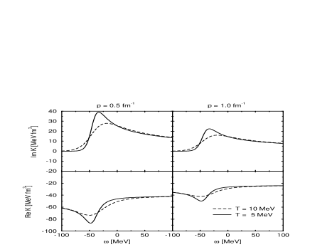
FIG. 3.: Real and imaginary part of the diagonal elements of the thermodynamic K-matrix (${}^{3}{\rm S}_{1}$) from Brueckner theory plotted for the same parameters as in Fig. 2.

However, with this difference in mind we can conclude that the pairing instability at $T=T_{c}$ is in qualitative agreement with the corresponding instability at $T=0$ observed in ref. [32]. However, a proper treatment of the pairing correlations below $T_{c}$ demands the inclusion of a finite gap in the single particle propagators. This has to be determined consistently from a combination of the BCS theory with the T-matrix approximation. Such a treatment known as quasiparticle-RPA [34] has recently been applied to the one-dimensional Fermi gas [35].

To compare with the Brueckner theory the respective key quantity is the K-matrix. In Fig. 3 the K-matrix elements of the Brueckner theory are given for the same set of parameters. The imaginary part of the K-matrix does not change sign in contrast to the T-matrix elements (Fig. 2). This is due to the fact that in this case the Pauli-blocking (19) is positive in contrast to the Pauli-blocking term (35), which changes sign at $2\epsilon(p)=2\mu$. For low temperatures the imaginary part is effectively zero for energies below this particular energy. For energies above this value a pronounced maximum develops. This gives the corresponding maximum in the real part of the K-matrix. However, no critical temperature can be found where the K-matrix diverges as found for the T-matrix (Thouless-criterion). Thus, the different Pauli operator (19) in the K-matrix leads to considerable deviations from the T-matrix case in particular in the limit of low temperatures.

In order to calculate the spectral function it is necessary to evaluate the off-shell selfenergy, which itself has some interesting features. In Fig. 4 the imaginary part of the retarded selfenergy (11) is given as a function of $\omega$ at $p_{1}=0$ and $n=n_{0}$. The results are plotted for various temperatures.

FIG. 4.: Imaginary part of the nucleon selfenergy (11) at the saturation density $n_{0}$ as a function of energy for momentum $p_{1}=0$. The selfenergy is given for several temperatures above the critical temperature for superfluidity ($T_{c}=4.02\;{\rm MeV}$). The chemical potential $\mu=-23.5\;{\rm MeV}$ ($T=4.1\;{\rm MeV}$) and the location of the pairing peak at $\omega_{0}=2\mu-\epsilon_{1}=35.6\;{\rm MeV}$ are indicated.

At the highest temperature $T=20\;{\rm MeV}$ (long-dashed curve) the selfenergy is rather smooth. It gives a non-zero contribution for energies $\omega>-200\;{\rm MeV}$, develops a maximum near $\omega=-100\;{\rm MeV}$ and then starts decreasing slowly. In the $T=10\;{\rm MeV}$ case we find two additional extrema: a minimum at the the chemical potential $\omega=\mu\approx-23\;{\rm MeV}$ and a second maximum at $\omega_{0}=2\mu-\epsilon(p_{1})\approx 35\;{\rm MeV}$. Decreasing the temperature further this behaviour gets still more pronounced. At the minimum the value of the imaginary part is drastically reduced; however it still has a finite value and will reach zero only in the limit $T\rightarrow 0$ (see discussion of Fig. 5). The second maximum gets more pronounced as well. At a temperature $T=4.1\;{\rm MeV}$, close to the critical temperature $T_{c}=4.02\;{\rm MeV}$, one observes a pronounced peak.

This particular behaviour can be traced back to the behaviour of the T-matrix (15) at low temperatures. It has been demonstrated in ref. [21] that ${\rm Im}\,T$ has a zero at the particular energy value $z=2\mu$ for pairs with zero total momentum (compare also Fig. 2). This compensates for the Bose singularity in the imaginary part of the selfenergy (11) rendering Im $\Sigma$ at this energy finite. However, in addition a critical temperature can be found such that the real part of the T-matrix becomes singular at the same energy (Fig. 2). As has been shown in Ref. [21] this critical temperature coincides with the one for the superfluid phase transition in agreement with the BCS theory. In fact, the singularity in the T-matrix is nothing but the wellknown Thouless criterion [20] for superfluidity. If this critical temperature is reached the above mentioned compensation does no longer hold (see also ref. [21]) and the singularity in the T-matrix leads to a corresponding singularity in the imaginary part of the selfenergy. The singularity is located at an energy $\omega_{0}=2\mu-\epsilon_{1}$. This is readily to be seen if one restricts to the pole part of the T-matrix with total momentum $P=0$. Then the integration over $p_{2}$ in (11) can be carried out directly yielding a $\delta$-peak in Im $\Sigma$ at the energy $\omega_{0}$. This shows that the singularity in the imaginary part of the selfenergy, which occurs for $T\rightarrow T_{c}$ is a direct consequence of the pole in the T-matrix at $T=T_{c}$, indicating the onset of superfluidity.

In Fig. 5 we continued the evaluation of the imaginary part of the selfenergy for temperatures below $T_{c}$, disregarding for the moment the pairing instability.

FIG. 5.: The same quantity as in Fig. 4 for temperatures below the critical temperature $T_{c}=4.02\;{\rm MeV}$. Again the chemical potential $\mu=-22.2\;{\rm MeV}$ ($T=1\;{\rm MeV}$) is indicated.

This allows us to demonstrate that for $T\rightarrow 0$ indeed the value of the imaginary part of $\Sigma$ at the minimum ($\omega=\mu=-23\;{\rm MeV}$) approaches zero, in accordance with zero temperature calculations of various authors [5, 36]. This zero of the imaginary part of the selfenergy at $\omega=\mu$ is a wellknown property at zero temperature leading to the fact that particles at the Fermi surface have infinite lifetime, i.e. they are good quasiparticles. According to the Hugenholtz-van-Hove theorem the chemical potential coincides with the binding energy per nucleon. The empirical value for this quantity at saturation is $E_{B}^{0}/A=-16\;{\rm MeV}$. The quadratic dependence of ${\rm Im}\,\Sigma$ around $\omega=\mu$ at $T=0$ demonstrated in ref. [37] is also found in our numerical calculations. With increasing temperature a non-zero value for ${\rm Im}\,\Sigma$ is obtained at $\omega=\mu$, however up to temperatures $T\leq 20\;{\rm MeV}$ (see Fig. 4) a pronounced minimum is reminiscent of the zero-temperature property. At all temperatures $T<T_{c}$ the pairing instability shows up at $\omega_{0}=2\mu-\epsilon_{1}=35\;{\rm MeV}$. This pairing instability indicates the breakdown of the T-matrix approximation in the vicinity of $\omega_{0}$ at temperatures below $T_{c}$. A consistent treatment requires the inclusion of the BCS-gap for temperatures below $T_{c}$. Such a complicated calculation has not yet been carried out. The $T=1\;{\rm MeV}$ curve in Fig. 5 is in qualitative agreement with the calculation of ref. [4] except at energies around $\omega\approx 35\;{\rm MeV}$. There we find the additional peak due to the pairing singularity in the T-matrix discussed above.

FIG. 6.: The imaginary part of the nucleon selfenergy at the saturation density calculated in Brueckner theory (eqs. (22)) for the same parameters as in Fig. 4.

In Fig. 6 the imaginary part of the selfenergy ${\rm Im}\,\Sigma_{\rm B}$ (22) is given as a function of energy for the same parameters as in Fig. 4. For $T=20\;{\rm MeV}$ ${\rm Im}\,\Sigma_{\rm B}$ is in qualitative agreement with the corresponding curve in Fig. 4. With decreasing temperature the qualitative behaviour is similar to the Green function case given in Fig. 4 except in the energy range around $\omega_{0}$. Whereas a strong singularity is seen in Fig. 4 for temperatures close to $T_{c}$ only a small maximum is found in the Brueckner case for the same temperature. As discussed above this singularity is due to the pairing singularity in the T-matrix and occurs at the critical temperature defined by the Thouless criterion. This behaviour does not show up in the Brueckner theory.

FIG. 7.: Direct comparison of the imaginary part of the selfenergy in Brueckner theory (dashed curves) and Green function theory (solid curves) for temperatures $T=20\mbox{ and }T=4.1\;{\rm MeV}$.

Fig. 7 gives a direct comparison between the imaginary parts of the selfenergy, calculated in the T-matrix and the Brueckner approximations, respectively. The upper curves show the case at $T=20\;{\rm MeV}$. While for energies below $\omega=-100\;{\rm MeV}$ and above $\omega=100\;{\rm MeV}$ the two curves almost coincide, the imaginary part of the Brueckner selfenergy lies below the one from the T-matrix calculation in the energy range between $-100\mbox{ and }100\;{\rm MeV}$. An analogous result has als been found in the zero-temperature case by Köhler [4]. In the $T=4.1\;{\rm MeV}$ case (slightly above $T_{c}$) we observe a similar relation between the two approximations. However, at energies around $\omega_{0}$ the Green function selfenergy shows the pairing singularity, which is absent in the Brueckner calculation.

In Fig. 8 the same quantity like in Fig. 4 is given using the Mongan potential instead of the Yamaguchi potential used throughout the rest of the paper. The purpose is to demonstrate the influence of the repulsive part of the nucleon-nucleon interaction on the selfenergy.

FIG. 8.: The imaginary part of the nucleon selfenergy at the saturation density for the Mongan NN-interaction. The critical temperature in this case has a smaller value ($T_{c}=1.58\;{\rm MeV}$) than for the Yamaguchi-potential. Like in Fig. 4 the selfenergy is given for several temperatures above and close to the critical temperature for superfluidity. The chemical potential $\mu=14.68\;{\rm MeV}$ and the energy $\omega_{0}=82.46\;{\rm MeV}$ is indicated. The inset shows the region around $\omega_{0}$ in detail.

The repulsion leads to a lower critical temperature ($T_{c}=1.58\;{\rm MeV}$) as compared to the barely attractive case ($T_{c}=4.02\;{\rm MeV}$). The temperature dependence of ${\rm Im}\,\Sigma$ does not change qualitatively compared to Fig. 4. Thus, we suppose that the behaviour discussed above also holds for more realistic interactions, such as the Paris-potential [38] as used e.g. in ref. [21].

FIG. 9.: The real part of the off-shell nucleon selfenergy calculated from the imaginary part according to eq. (13) as a function of energy for $n=n_{0}$ and the same temperatures as in Fig. 4.

In addition to the imaginary part the real part of the selfenergy contains important information, its on-shell part defining the optical potential for the nucleon in nuclear matter. In Fig. 9 the energy dependence of the real part of the selfenergy as calculated from eq. (13) is shown for the same parameters as used in Fig. 4. Again there is a relatively smooth behaviour for the $=20\;{\rm MeV}$ case. With decreasingtemperature a second minimum is found for energies below $\omega_{0}$. Please note that for $T=4.1\;{\rm MeV}$ (close to $T_{c}=4.02\;{\rm MeV}$) a principle-value-like behaviour around $\omega=\omega_{0}$ is found. This a direct consequence of the corresponding pairing peak in the imaginary part of the selfenergy at $\omega=\omega_{0}$ (see Fig. 4).

In Fig. 10 the real part of the on-shell self energy i.e. the real part of the optical potential, is given as a function of the momentum $p$. The upper curve shows a calculation using only the first term in eq. (12). This is a standard approximation often used to calculate the optical potential in nuclear matter [13, 39, 40].

FIG. 10.: The real part of the on-shell nucleon selfenergy as a function of the momentum $p$ for $n=n_{0}$ and different temperatures according to eq. (12). The upper figure was a calculation using only the first term of eq. (12) denoted as ${\rm Re}\,\Sigma^{1}$. The lower plot shows the result of the full expression. The Fermi-momentum is indicated as $p_{\rm F}$.

With decreasing temperature one observes a pronounced minimum near the Fermi energy, which has first been observed in ref. [13] and related to the inclusion of hole-hole scattering in the Pauli operator. However, using the full expression of eq. (12) for the evaluation of the optical potential the behaviour at low temperatures is changed. A particular structure is found around momenta $p=p_{\rm F}$ which is enhanced with decreasing temperature. If one studies the behaviour of the real part in detail, one finds, that the ${}^{3}{\rm S}_{1}$-channel of the T-matrix is responsible for this anomalous behaviour. We suppose, that the pairing peak in the imaginary part ${\rm Im}\,\Sigma(p,\omega)$ at temperatures $T\rightarrow T_{c}$, present also at finite momenta $p$, leads to a corresponding principal-value-like structure in the real part of the optical potential. Restricting to the pole part of the T-matrix this behaviour can be shown using the dispersion relation between the real and imaginary parts of the selfenergy. Consequently for the on-shell selfenergy ${\rm Re}\,\Sigma$ this leads to the wiggle at $p=p_{\rm F}$.

Fig. 11 shows the same quantity calculated from the Brueckner theory. The upper plot denoted as ${\rm Re}\,\Sigma_{\rm B}^{1}$ shows the temparature behaviour of the first order Brueckner term (eq. (23)). For the lowest temperature ($T=4.1\;{\rm MeV}$) one observes a plateau-like behaviour around the Fermi momentum. Using the full expressions (lower plot) the repulsive second order contribution leads to a different behaviour at low temperatures, which is characterized by a strong enhancement for low momenta and a corresponding minimum for momenta $p>p_{\rm F}$.

FIG. 11.: The real part of the on-shell nucleon selfenergy calculated with the Brueckner K-matrix. The parameters are the same as in Fig. 10. While the upper figure shows the results only with the first term of eq. (23) denoted as ${\rm Re}\,\Sigma_{\rm B}^{1}$ the lower part shows the results of the full calculation.

A particular behaviour of the optical potential for momenta around $p=p_{\rm F}$ has also been found in refs.[39, 41]. In ref. [41] a plateau-like behaviour was related to the behaviour of the effective mass at the Fermi surface. In [39] it was shown that a non-monotonous behaviour around $p_{\rm F}$ (anomaly) was entirely due to the strong attraction in the ${}^{3}{\rm S}_{1}-{}^{3}{\rm D}_{1}$ channel and that it was enhanced if the density was decreased below $n=n_{0}$. According to our understanding the anomaly observed in ref. [39] is probably as well due to the pairing instability [42] discussed above.

FIG. 12.: The real part of the on-shell nucleon selfenergy calculated in T-matrix and Brueckner approximations, respectively, for temperature $T=30\;{\rm MeV}$.

In Figs. 12-14 we give a direct comparison between the Green function theory and Brueckner theory with respect to the real part of the on-shell selfenergy for different temperatures. The upper curves correspond to the first term in eqs. (12) and (23), respectively. As the form of these expressions coincides, the differences between Green function and Brueckner theory in this case are entirely due to the different Pauli operators in the T-matrix and K-matrix, respectively (compare eq. (19). The lower curves show the result of the full expressions (12) and (23). In Fig. 12 we give the results for temperature $T=30\;{\rm MeV}$. The differences between the two approaches are not very pronounced for this temperature, except for low momenta. With respect to ${\rm Re}\,\Sigma^{1}$ the Green-function-curve is slightly enhanced compared to the Brueckner-curve for momenta $p\simeq p_{\rm F}$ and slightly reduced below. This behaviour is reversed for the lower curves.

FIG. 13.: The same figure as Fig. 12 for temperature $T=10\;{\rm MeV}$.

In Fig. 13 ($T=10\;{\rm MeV}$) the differences between the two theories are much more pronounced. The different form of the Pauli operarator results in a non-monotonous behaviour for the Green function curve showing a pronounced minimum around $p=p_{\rm F}$. In contrast the Brueckner curve is monotonously decreasing. A behaviour like this has first been observed in ref. [13]. For the full expressions the differences between both theories are less pronounced showing an enhancement of the Green function curve with respect to the Brueckner curve for momenta $p<p_{\rm F}$.

FIG. 14.: The same figure as Fig. 12 for temperature $T=4.1\;{\rm MeV}$.

In Fig. 14 the temperature ($T=4.1\;{\rm MeV}$) is close to the critical temperature $T_{c}=4.02\;{\rm MeV}$. One observes basically the same behaviour as in Fig. 13, although the differences are still more enhanced.

In Fig. 15 the imaginary part of the on-shell selfenergy (optical potential) is given as a function of momentum for various temperatures. The upper graph shows the contribution of the first term in eq. (11) only.

FIG. 15.: The imaginary part of the on-shell selfenergy as a function of $p$ at $n_{0}$ for the same temperatures as in Fig. 10, according to eq. (11). The upper figure was a calculation using only the first term of eq. (11) denoted as ${\rm Im}\,\Sigma^{1}$. The lower plot shows the result of the full expression. The Fermi-momentum is indicated as $p_{\rm F}$.

One observes a pronounced temperature dependence for momenta below $p=2\;{\rm fm}^{-1}$ leading to a decrease with temperature towards a minimum near $p=p_{\rm F}$. The lower graph displays the full contribution for the imaginary part (11). Again, one notes a strong temperature dependence below $p=2\;{\rm fm}^{-1}$. For momenta around the Fermi momentum a pronounced minimum is exhibited with decreasing temperature. The value of ${\rm Im}\,\Sigma$ at $p=p_{\rm F}$ tends to zero for $T\rightarrow 0$.

FIG. 16.: The imaginary part of the on-shell nucleon selfenergy calculated with the Brueckner K-matrix. The parameters are the same as in Fig. 15. The upper figure shows the results only with the first term of eq. (22) denoted as ${\rm Im}\,\Sigma_{\rm B}^{1}$. The lower part shows the results of the full calculation (22).

In Fig. 16 the imaginary part of the on-shell selfenergy calculated in Brueckner theory ${\rm Im}\,\Sigma_{\rm B}$ is given as a function of momentum for the same parameters as in Fig. 15. The upper plot displays the first term of eq. (22). Again, we observe a strong decrease with temperature for momenta below $p=2\;{\rm fm}^{-1}$ as in figure 15. However, due to the use of the different Pauli-operator in the K-matrix ${\rm Im}\,\Sigma_{\rm B}^{1}$ is basically zero for momenta $p<p_{\rm F}$ in the limit of low temperatures. No minimum can be observed. In the lower graph the full contribution of ${\rm Im}\,\Sigma_{\rm B}$ (22) is shown. One notes, that the temperature dependence for momenta around $p_{\rm F}$ is in qualitative agreement with the Green function result (lower curve of Fig. 15). However, for momenta $p\leq 1\;{\rm fm}^{-1}$ the temperature behaviour is reversed compared to the Green function case. Please note, that it is in the same momentum range, where one notes pronounced deviations in the real part of the optical potential at low temperatures (compare lower part of Fig. 14). The Brueckner results can be compared with the calculation of ${\rm Im}\,V_{\rm B}(1,\epsilon_{1})$ in ref. [10]. Taking into account the relation between ${\rm Im}\,\Sigma_{\rm B}$ and ${\rm Im}\,V_{\rm B}$ (see sect. III) one notes the qualitative agreement of the two calculations.

Summarizing, one observes pronounced differences between the optical potential at low temperatures calculated in Green-function-theory and Brueckner theory, respectively. These show up at momenta below the Fermi momentum. For the full expressions (lower curves) these differences are due to higher order terms in the Green-function-approximation, not included in the second order Brueckner calculation (see also ref. [25]).

V Spectral function and momentum distributions

From the off-shell selfenergy the nucleon spectral function is calculated using eq. (1). In Fig. 17 the nucleon spectral function is plotted as a function of energy $\omega$ for zero momentum $p_{1}=0$ at a density $n=n_{0}$ and for the same temperatures as given in Fig. 4. For $T=20\;{\rm MeV}$ one observes a quasiparticle peak at energies $\omega=-150\;{\rm MeV}$ and a background contribution extending up to energies $\omega\approx 200\;{\rm MeV}$.

FIG. 17.: The nucleon spectral function at the saturation density as a function of energy for momentum $p_{1}=0$. The temperatures are the same as in Fig. 4.

With decreasing temperature the quasiparticle peak is slightly shifted towards higher energies and its width is reduced. This reduction is due to the fact that with decreasing temperature the imaginary part reaches zero at higher energies (compare Fig. 4). In addition a second maximum forms at lower energies. This can be compared with the zero temperature results in ref. [4] for the spectral function at $p=0$. Using Green function theory they also arrive at a spectral function with two peaks of comparable size which are located at approximately the same energies as given in Fig. 17. in the $T=4.1\;{\rm MeV}$ case.

The temperature dependence of the spectral function is not as drastic as one could expect from the change in the selfenergy with temperature (Fig. 4). Near the critical temperature the tail of the spectral function at higher energies shows additional smaller maxima, which result from the pronounced structures in the real part of the selfenergy. These in turn are due to the singular behaviour of the imaginary part at $\omega=2\mu-\epsilon_{1}$.

FIG. 18.: The nucleon spectral function at saturation density and $T=10\;{\rm MeV}$ in the energy-momentum plane.

In Fig. 18 the energy and momentum dependence of the spectral function is given at $n=n_{0}$ and $T=10\;{\rm MeV}$. One observes that the double-peak structure found at $p=0$ vanishes with increasing momentum. A single maximum remains for $p_{1}>0.7\;{\rm fm}^{-1}$ which can be identified with the quasiparticle peak. The width of this peak is reduced at $p=p_{\rm F}$ due to the minimum in ${\rm Im}\,\Sigma$ at the chemical potential. For larger momenta the peaks are broadened again until for very high momenta the width is reduced again. The latter behaviour is due to the fact that for very high momenta the influence of the medium represented by the selfenergy becomes negligible. Please note, that for our choise of the nucleon-nucleon-interaction there is no high-momentum tail of the spectral function, because it is barely attractive.

In order to demonstrate the influence of correlations on the nucleon occupation numbers, the spectral function can be used to determine this quantity. In Fig. 19 the temperature dependence of the nucleon momentum distribution (occupation numbers) $n(p)$ (3) is given at a fixed density $n=n_{0}$. The correlated occupation number (full line) is compared to the corresponding Fermi distribution function (dashed line). In the $T=5\;{\rm MeV}$ case we observe a strong depletion for momenta below the Fermi momentum with a value of $n(p=0)=0.78$ compared to 1 for the non-interacting case. Above the Fermi surface we find a corresponding enhancement of the interacting occupation numbers compared to the non-interacting up to about $p=2\;{\rm fm}^{-1}$. For $T=10\;{\rm MeV}$ the depletion is less pronounced ($n(0)=0.82$). This tendency towards the non-interacting occupation numbers is continued is the case of $T=30\;{\rm MeV}$. With further increasing temperature the interacting response approaches the non-interacting one. Using the Brueckner K-matrix in ref. [43] the finite temperature occupation numbers are evaluated which are in reasonable aggreement with our results as well with the calculations of ref. [10].

In Fig. 20 the density dependence of $n(p)$ at fixed $T$ ($10\;{\rm MeV}$) is shown. For the sake of a better comparability the curves are normalized to $p/p_{\rm F}$. When going to densities above $n_{0}$ ($n/n_{0}=1.32$) one observes a lower depletion ($n(p=0)=0.85$) compared to $n(p=0)=0.82$ at $n=n_{0}$.

FIG. 19.: Occupation numbers at saturation density for different temperatures. The dashed curves represent the uncorrelated occupation numbers, i.e. the corresponding Fermi distribution.

The same tendency has also been observed in ref. [43], although at a higher temperature ($30\;{\rm MeV}$). Going to lower densities ($n/n_{0}=0.61$) we find the astonishing result that the depletion at low $p$ is further enhanced ($n(p=0)=0.78$).

FIG. 20.: Occupation numbers at $T=10\;{\rm MeV}$ for density values around the saturation density. Again the dashed curves represent the non-interacting case.

On the other hand this corresponds to the zero temperature results of ref. [7, 8] indicating that the momentum distribution does not approach the non-interacting one in the limit of zero density. In ref. [8] the depletion at $T=0$ and $p=0$ stays rather constant for densities between $n_{0}$ and $n_{0}/2$ at a value of $n(p=0)=0.86$. The authors of ref. [8] interpret this result as being due to the attractive part of the nucleon-nucleon-interaction leading to the formation of bound pairs at low densities.

VI Summary and Conclusions

Using the Matsubara Green function approach, selfconsistent expressions for the nucleon selfenergy and the nucleon spectral function for nuclear matter at finite temperature were derived. The selfenergy and the nucleon spectral function at the saturation density were calculated in first iteration starting from the quasiparticle spectral function. The variation of these quantities with temperature was studied for temperatures close to the critical temperature $T_{c}$ for the superfluid phase transition in symmetric nuclear matter. We found that approaching the critical temperature from above a singularity develops in the imaginary part of the selfenergy. It was shown that this singularity is a direct consequence of a corresponding pole in the T-matrix at the energy $E=2\mu$, which indicates the onset of a superfluid phase at $T=T_{c}$ [20]. Thus, the modification of the selfenergy near $T_{c}$ can be understood as a precursor effect of the superfluid phase transition in nuclear matter. Another effect which was discussed as being related to the pairing instability in the ${}^{3}{\rm S}_{1}-{}^{3}{\rm D}_{1}$-channel is the occurrence of a wiggle around $p=p_{\rm F}$ in the real part of the on-shell selfenergy, especially pronounced when approaching $T_{c}$ from above. A similar effect although less pronounced was also found in the Brueckner calculation.

The temperature dependence of the spectral function has been investigated for temperatures above the critical temperature. Despite the strong modification of the selfenergy there is no such drastic modification of the spectral function when approaching $T_{c}$ from above. This is consistent with the fact that below $T_{c}$ the condensate part of the T matrix is proportional to the square of the gap and consequently vanishes at the critical temperature.

The momentum dependence of the spectral function shows considerable deviations from the quasiparticle behaviour at small momenta, whereas the quasiparticle picture holds approximately for momenta around $p=p_{\rm F}$ as well as for large $p$.

The occupation numbers were calculated from the spectral function at some finite temperature and density. It could be shown that with increasing temperature the non-interacting occupation number is approached. The depletion of the occupation numbers is enhanced with decreasing density at finite temperature.

At the end we would like to mention some open questions related to our calculation of the nucleon spectral function: The first question is related to the model interaction we used in our exploratory calculation of the selfenergy and spectral function. For the energy and momentum range investigated in this paper the important features of the selfenergy obtained using the simple model interaction of Yamaguchi type were also found using a rank two Mongan interaction. It is supposed that these features remain of relevance also for more realistic potentials [38].

The second question is related to the problem of selfconsistency. In principle, the spectral functions have to be iterated until selfconsistency is reached. It remains to be seen, to what extent the features of the first iteration obtained in this calculation will also be found in a fully selfconsistent calculation.

The third question concerns a consistent description of the system below $T_{c}$, where the consistent inclusion of a finite gap is necessary for the evaluation of the spectral function. In principle our calculation is restricted to temperatures above the critical temperature for superfluidity. The Thouless criterion indicates the instability of the normal quasiparticle state with respect to the onset of superfluidity. A consistent treatment below $T_{c}$ has to be based e.g. on a BCS quasiparticle basis with a finite gap. Up to now such a calculation has not been carried out for nuclear matter. Instead, in most of the approaches at zero temperature the implications of the pairing singularity for the selfenergy were neglected. However, in a series of papers Dickhoff et al. [5] stressed the need to properly take into account the T matrix singularity, discussed above, which is present at temperatures below $T_{c}$.

In conclusion we evaluated the nucleon self energy and spectral function for finite temperature. We compared the calculations within the Green function approach with a finite temperature generalization of the Brueckner theory. Special emphasis was put on the behaviour of these quantities near the critical temperature for the onset of superfluidity in nuclear matter. Within the Green function approach the pairing singularity in the T-matrix at the critical temperature generates a corresponding singularity in the imaginary part of the selfenergy. The non-monotonous behaviour (anomaly) of the real part of the optical potential for momenta $p\sim p_{\rm F}$ could also be related to the pairing singularity. The spectral function at finite temperature shows a complex energy dependence, which cannot be generated from an energy-independent width.

All the features discussed above cannot be incorperated into a simple quasiparticle description. Thus, the nucleon spectral function should be the appropriate quantity for the description of hot and dense nuclear matter.

REFERENCES

- [1] O. Benhar, A. Fabrocini, S. Fantoni, G.A. Miller, V.R. Pandharipande and I. Sick, Phys. Rev. C 44, 2328 (1991) (and references therein).
- [2] O. Benhar, A. Fabrocini, S. Fantoni, Nucl. Phys. A 505, 267 (1989).
- [3] M. Baldo, I. Bombaci, G. Giansiracusa, U. Lombardo, C. Mahaux and R. Sator, Nucl. Phys. A 545, 741 (1992).
- [4] H.S. Köhler, Phys. Rev. C 46, 1687 (1992).
- [5] B.E. Vonderfecht, W.H. Dickhoff, A. Polls and A.Ramos, Nucl. Phys. A 555, 1 (1993).
- [6] O. Benhar, A. Fabrocini, and S. Fantoni, Nucl. Phys. A 505, 267 (1989).
- [7] O. Benhar, A. Fabrocini, S. Fantoni, I. Sick, Nucl. Phys. A 579, 493 (1994).
- [8] D. Van Neck, A.E.L. Dieperink, E. Moya de Guerra, Phys. Rev. C 51, 1800 (1995).
- [9] F. de Jong and R. Malfliet, Phys. Rev. C 44, 998 (1991).
- [10] P. Grangé, J. Cugnon and A. Lejeune, Nucl. Phys. A 473, 365 (1987).
- [11] G. Röpke, L. Münchow and H. Schulz, Nucl. Phys. A 379, 536 (1982).
- [12] H.S. Köhler, Nucl. Phys. A 529, 209 (1991).
- [13] M. Schmidt, G. Röpke and H. Schulz, Ann. Phys. (N.Y.) 202 , 57 (1990).
- [14] T. Alm, G. Röpke, A. Schnell and H. Stein, Phys. Lett. B 346, 233 (1995).
- [15] T. Alm, B.L. Friman, G. Röpke, and H. Schulz, Nucl. Phys. A 551, 45 (1993).
- [16] H.F. Areanello, F.A. Brieva and W.G. Love, Phys. Rev. C 50, 2480 (1994).
- [17] M. Baldo, I. Bombaci and U. Lombardo, Phys. Lett. B 283, 8 (1992).
- [18] H. Stein, A. Schnell, T. Alm and G. Röpke, Z. Phys. A 351, 295 (1995).
- [19] M. Baldo, U. Lombardo and P. Schuck, Phys. Rev. C 52, 975 (1995).
- [20] D.J. Thouless, Ann. Phys. (N.Y.) 10, 553 (1960).
- [21] T. Alm, G. Röpke and M. Schmidt, Phys. Rev. C 50, 31 (1994).
- [22] A.L. Fetter and J.D. Walecka, Quantum Theory of Many-Particle Systems, McGraw-Hill (1971).
- [23] W.D. Kraeft, D. Kremp, W. Ebeling and G. Röpke, Quantum Statistics of Charged Particle Systems Plenum N.Y. (1986).
- [24] C. Bloch and C. De Dominicis, Nucl. Phys. 7,459 (1958), Nucl. Phys. 10,181 (1959), Nucl. Phys. 10,509 (1959).
- [25] H.S. Köhler and R. Malfliet, Phys. Rev. C 48, 1034 (1993).
- [26] P. Danielewicz, Ann. Phys. 197, 154 (1990).
- [27] H. S. Köhler and R. Malfliet, Acta Phys. Polonica B24, 513 (1993).
- [28] W. Botermans and R. Malfliet, Phys. Rep. 198, 115 (1990).
- [29] J. Cugnon, P. Grangé and A. Lejeune, J. de Phys., Colloq. C2, 281 (1987).
- [30] Y. Yamaguchi, Phys. Rev. 95, 1628 (1954).
- [31] T. R. Mongan, Phys. Rev. 178, 1597 (1969).
- [32] A. Ramos, A. Polls and W.H. Dickhoff, Nucl. Phys. A 503, 1 (1989).
- [33] Kadanoff and G. Baym, Quantum Statistical Mechanics, Benjamin, New York (1962).
- [34] P. Ring, P. Schuck, The Nuclear Many-Body Problem, Springer N.Y. (1980).
- [35] T. Alm and P. Schuck, (submitted to Phys. Rev. B).
- [36] M. Baldo, I. Bombaci, G. Giansiracusa, U. Lombardo, C. Mahaux and R. Sartor, Phys. Rev. C 41, 1748 (1990).
- [37] J.P. Blaizot and B.L. Friman, Nucl. Phys. A 372, 69 (1981).
- [38] L. Mathelitsch, W. Plessas and W. Schweiger, Phys. Rev. C 26, 65 (1982).
- [39] N. Yamaguchi, S. Nagata and T. Matsuda, Prog. Theor. Phys. 70, 459 (1983).
- [40] A. Lejeune, P. Grangé, M. Martzloff and J. Cugnon, Nucl. Phys. A 453, 189 (1986).
- [41] V. Bernard and C. Mahaux, Phys. Rev. C 23, 888 (1981).
- [42] A. Ramos, W.H. Dickhoff and A. Polls, Phys. Rev. C 43, 2239 (1991).
- [43] H.S. Köhler, Nucl. Phys. A 537, 64 (1992).