Multipole analysis of spin observables in vector meson photoproduction

Abstract

A multipole analysis of vector meson photoproduction is formulated as a generalization of the pseudoscalar meson case. Expansion of spin observables in the multipole basis and behavior of these observables near threshold and resonances are examined.

I Introduction

With the advent of CEBAF there is renewed interest in measuring the photoproduction of vector mesons $(\rho,\omega,\phi)$ [3, 4]. In anticipation of such experiments, the general nature of spin observables for vector mesons has been studied[5] using a helicity amplitude approach. In this paper, that study is extended by introducing electric and magnetic multipole amplitudes for the photoproduction of vector mesons. The multipoles include the final state orbital angular momentum and thus, near threshold, provide a natural truncation to relatively few multipoles. Also, since resonances have definite $\ell$-values, the isolation of isobar dynamics occurs most naturally in a resonant multipole amplitude. Expressions for the full array of spin observables in terms of these multipoles are derived. Then, general rules for the angular dependence of these observables and their dependence on multipoles are discussed. We hope that such rules will be helpful in analyzing future experiments.

II Multipoles For vector meson production

The general structure of the scattering amplitude for the photoproduction of vector mesons is:

$$<\vec{q}\,\lambda_{V}\,m_{2}\mid T\mid\vec{k}\, \lambda_{\gamma} \,m_{1}>$$ (1)

$$\equiv \hat{\varepsilon}_{\lambda_{V}}^{*}(\vec{q}\,)\cdot<m_{2}\mid\stackrel{{\scriptstyle\leftrightarrow}}{{J}}\mid m_{1}>\cdot\hat{\varepsilon}_{\lambda_{\gamma}}(\vec{k}\,)$$ (2)

$$\equiv <m_{2}\mid{\cal J}_{\lambda_{V}\lambda_{\gamma}}\mid m_{1}>,$$ (3)

where $\vec{k},\lambda_{\gamma}$ and $\vec{q},\lambda_{V}$ denote the three-momentum and helicity of the initial photon and final vector meson; $m_{1}$ and $m_{2}$ are the initial and final nucleon spins quantized along the $z$-axis, respectively ( see Fig. 1). Isospin factors are suppressed.

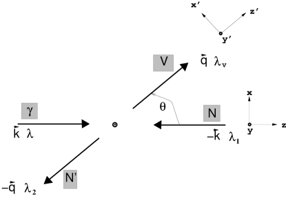
FIG. 1.: The coordinate system and kinematical variables for vector meson photoproduction. Here V denotes the vector meson and $\lambda_{V}$ its helicity.

The current tensor $\stackrel{{\scriptstyle\leftrightarrow}}{{J}}$ is defined in the Pauli-spinor space of the initial and final baryon. One can express this current in terms of 12 generalized CGLN amplitudes[6], and proceed to find an expansion of those amplitudes in terms of multipoles. Reference [7] gives the transformation matrices connecting helicity amplitudes to a set of gauge invariant covariant amplitudes for this reaction. In our paper, we follow a direct approach to relate helicity amplitudes to multipoles, without using CGLN amplitudes as an intermediate step.

A Multipole amplitudes

The quantum numbers introduced in the multipole analysis are: the total angular momentum $J$ and its projection along the $z$-axis $M,$ the relative orbital angular momentum $\ell_{V}$ of the final particles; the total angular momentum of the final vector particle $j_{V}$ and of the initial photon $j_{\gamma}$ with respect to the nucleon; and the multipole type of the photon $\phi_{\gamma}.$ Here, $\phi_{\gamma}$ denotes either electric $\phi_{\gamma}=E(j_{\gamma}=\ell_{\gamma}\pm 1)$ or magnetic $\phi_{\gamma}=M(j_{\gamma}=\ell_{\gamma})$ multipole type.

Introducing complete sets of initial and final angular momentum states, the $T$ matrix element can be brought into the following form:

$$<\vec{q}\,\lambda_{V}\,m_{2}\mid T \mid\vec{k}\,\lambda_{\gamma}\,m_{1}>$$ (5)

$$=\sum_{\alpha}<m_{2}\mid{\cal P}^{\lambda_{V}\lambda_{\gamma}}_{\alpha}\mid m_{1}>T_{\alpha}\ .$$

In other words:

$${\cal J}_{\lambda_{V}\lambda_{\gamma}}=\sum_{\alpha}{\cal P}^{\lambda_{V}\lambda_{\gamma}}_{\alpha}\ T_{\alpha}\ ,$$ (6)

where $\alpha\equiv(J,j_{V},\ell_{V},j_{\gamma},\phi_{\gamma}).$ The multipole amplitude $T_{\alpha}$ and the transformation operator ${\cal P}^{\lambda_{V}\lambda_{\gamma}}_{\alpha}$ are defined as

$$T_{\alpha}\equiv<(\ell_{V}1)(j_{V}\frac{1}{2})\,JM\mid T\mid(j_{\gamma}\frac{1}{2})\,\phi_{\gamma}\,JM>,$$ (7)

and

$$<m_{2}\mid{\cal P}^{\lambda_{V}\lambda_{\gamma}}_{\alpha}\mid m_{1}>\equiv\sum_{M}<\vec{q}\,\lambda_{V}\,m_{2}\mid q\,(\ell_{V}1)\,(j_{V}\frac{1}{2})\,JM><k\,\phi_{\gamma}\,(j_{\gamma}\frac{1}{2})\,JM\mid\vec{k}\,\lambda_{\gamma}\,m_{1}>.$$ (8)

Note that $T_{\alpha}$ is independent of $M.$ As seen above, the quantum numbers describing the initial and final states are quite similar, which is natural since both contain a vector particle($\gamma$ or $V$) and a nucleon. The only asymmetry in the quantum numbers is the use of $\ell_{V}$ in the final state instead of photon multipole type $\phi_{\gamma}.$ Coupling of angular momenta, which is implied by the use of parenthesis in the above expression, is pictured in Figure 2:

FIG. 2.: Final State Angular Momenta Addition

A plane wave photon state $|\vec{k}\,\lambda_{\gamma}>$ is characterized by its momentum $\vec{k}$ and helicity $\lambda_{\gamma}.$ A multipole photon state $|j_{\gamma}\,m_{\gamma},\phi_{\gamma}>$ is characterized by its total angular momentum $j_{\gamma}$ and its projection onto a fixed $\hat{z}$ axis, $m_{\gamma},$ and the multipole type $\phi_{\gamma}.$ The overlap of a photon plane wave state of definite helicity with a photon multipole state is given by:

$$<j_{\gamma}\,m_{\gamma}\,\phi_{\gamma}\mid\vec{k}\,\lambda_{\gamma}>=-\xi_{\phi_{\gamma}}\sqrt{\frac{2j_{\gamma}+1}{8\pi}}\,{\cal D}^{(j_{\gamma})}_{m_{\gamma}\lambda_{\gamma}}(\hat{k}),$$ (9)

where $\xi_{\phi_{\gamma}}$ is $1(\lambda_{\gamma})$ for Electric(Magnetic) multipoles, respectively. (We follow the phase convention of Ref [10] for the photon multipole state.) Using this expression, matrix elements of the transformation operator ${\cal P}$ can be simplified as:

$$<m_{2}\mid{\cal P}^{\lambda_{V}\lambda_{\gamma}}_{\alpha}\mid m_{1}>=C^{\lambda_{V}\lambda_{\gamma}}_{\alpha}(-1)^{\lambda_{V}}\sum_{m_{\gamma}m_{V}M}{\cal D}^{(j_{V})*}_{m_{V}\lambda_{V}}(\hat{q})$$ (10)

$$\times{\cal D}^{(j_{\gamma})}_{m_{\gamma}\lambda_{\gamma}}(\hat{k})\left(\begin{array}[]{ccc}j_{V}&1/2&J\\ m_{V}&m_{2}&-M\end{array}\right)\left(\begin{array}[]{ccc}j_{\gamma}&1/2&J\\ m_{\gamma}&m_{1}&-M\end{array}\right).$$ (15)

All angular momentum constraints are stored in the Wigner ${\cal D}$’s and in the three-$j$ symbols. In the above expression, $C$ is given by:

$$C^{\lambda_{V}\lambda_{\gamma}}_{\alpha}=\frac{(-1)^{j_{\gamma}-\lambda_{\gamma}}}{2\sqrt{2}\pi}\xi_{\phi_{\gamma}}(J+\frac{1}{2})$$ (16)

$$\times\sqrt{(2j_{V}+1)(2\ell_{V}+1)(2j_{\gamma}+1)}\left(\begin{array}[]{ccc}\ell_{V}&1&j_{V}\\ 0&-\lambda_{V}&\lambda_{V}\end{array}\right).$$ (19)

B Helicity and multipole amplitudes

In order to express the multipole amplitudes in terms of the helicity amplitudes, we need to invert Eq. (5). Therefore, an orthogonality relationship for the transformation operator ${\cal P}$ is needed. The operator ${\cal P}$ obeys the following orthogonality property:

$$\int\int d\Omega_{\hat{q}}\,d\Omega_{\hat{k}}\sum_{m_{1}m_{2}\lambda_{\gamma}\lambda_{V}}<m_{2}\mid{\cal P}^{{\dagger}\lambda_{V}\lambda_{\gamma}}_{\alpha}\mid m_{1}>$$ (20)

$$\times<m_{1}\mid{\cal P}^{\lambda_{V}\lambda_{\gamma}}_{\alpha^{\prime}}\mid m_{2}>=(2J+1)\delta_{\alpha\alpha^{\prime}}.$$ (21)

Using this property, Eq. (5) can be inverted to yield the multipole amplitudes:

$$T_{\alpha}=\frac{1}{2J+1}\int\int d\Omega_{\hat{q}}\,d\Omega_{\hat{k}}\sum_{m_{1}m_{2}\lambda_{\gamma}\lambda_{V}}$$ (22)

$$\times<m_{1}\mid{\cal P}^{{\dagger}\lambda_{V}\lambda_{\gamma}}_{\alpha}\mid m_{2}><\vec{q}\lambda_{V}m_{2}\mid T\mid\vec{k}\lambda_{\gamma}m_{1}>.\$$ (23)

Equations (21,23) remain valid when $m$’s(nucleon spin projections along the $z$-axis) are replaced by the nucleon helicities $\lambda$’s. Matrix elements of ${\cal P}$ in a nucleon helicity basis can be generated readily by Wigner rotations of the initial and final nucleon states. Such nucleon helicity-based projection operators can be used to relate the helicity and multipole amplitudes. The explicit expression is:

$$<\lambda_{N^{\prime}}\mid{\cal P}^{\lambda_{V}\lambda_{\gamma}}_{\alpha}\mid\lambda_{N}>=C^{\lambda_{V}\lambda_{\gamma}}_{\alpha}\sum_{M^{\prime}s}{\cal D}^{(J)*}_{M^{\prime\prime}M^{\prime}}(\hat{q})$$ (24)

$$\times{\cal D}^{(J)}_{M^{\prime\prime}M}(\hat{k})\left(\begin{array}[]{ccc}j_{V}&1/2&J\\ \lambda_{V}&-\lambda_{N^{\prime}}&-M^{\prime}\end{array}\right)\left(\begin{array}[]{ccc}j_{\gamma}&1/2&J\\ \lambda_{\gamma}&-\lambda_{N}&-M\end{array}\right).$$ (29)

As a result, it is found that the multipole amplitudes are directly related to the partial wave helicity amplitudes $<\lambda_{V}\lambda_{N^{\prime}}\mid T^{J}\mid\lambda_{\gamma}\lambda_{N}>$ by:

$$T_{\alpha}=\frac{4\pi}{2J+1}\sum_{\lambda_{\gamma}\lambda_{V}\lambda_{N}\lambda_{N^{\prime}}}C^{\lambda_{V}\lambda_{\gamma}}_{\alpha}\left(\begin{array}[]{ccc}j_{V}&1/2&J\\ \lambda_{V}&-\lambda_{N^{\prime}}&-\Lambda_{f}\end{array}\right)$$ (32)

$$\times\left(\begin{array}[]{ccc}j_{\gamma}&1/2&J\\ \lambda_{\gamma}&-\lambda_{N}&-\Lambda_{i}\end{array}\right)<\lambda_{V}\lambda_{N^{\prime}}\mid T^{J}\mid\lambda_{\gamma}\lambda_{N}>.$$ (35)

Although $T$ is labeled by five quantum numbers, $j_{\gamma}$ is dictated by parity, once the other quantum numbers are specified. This property follows since the initial and final state parities are respectively $-(-1)^{j_{\gamma}+\Phi}$ and $-(-1)^{\ell_{V}}$ where $\Phi$ is 0(1) for Magnetic(Electric) multipoles, or from Eq. (35) it is seen that

$$T_{\alpha}\sim 1+(-1)^{\ell_{V}+j_{\gamma}+\Phi}.$$ (36)

This result guarantees that there are at most 12 nonzero multipole amplitudes for any $J.$ For a given $J,$ there may be at most two different $j_{V}$’s $(J\pm\frac{1}{2}),$ three different $l_{V}$’s $(j_{V},j_{V}\pm 1),$ two different $j_{\gamma}$’s $(J\pm\frac{1}{2})$ and two multipole types $\Phi=0,1.$ Thus, the total number of possible multipole amplitudes is $2\times 3\times 2\times 2=24.$ Looking at the Eq. (36), one sees that for each set of quantum numbers either $\Phi=0$ or $\Phi=1$ gives a nonzero multipole amplitude. Therefore, one deduces that there are 12 complex multipole amplitudes for vector meson photoproduction. On the other hand, there are 24 complex helicity matrix elements. Since they are interrelated by parity invariance, only 12 helicity amplitudes are linearly independent.

C Labeling of multipole amplitudes

We now define multipole amplitudes for vector meson photoproduction by generalizing the notation used for pseudoscalar meson production. As in the pseudoscalar meson case, the labels $E,M$ are used to denote electric and magnetic multipoles. But for vector meson photoproduction, an additional $\pm,0$ designation is used to indicate how the vector meson’s orbital angular momentum is added to its spin. The generalization of the multipoles notation to the vector meson case is therefore:

$$E^{2(J-\ell_{\pi})}_{\ell_{\pi}} \longrightarrow E^{2(J-j_{V})}_{\ell_{V},(j_{V}-\ell_{V})},$$ (37)

$$M^{2(J-\ell_{\pi})}_{\ell_{\pi}} \longrightarrow M^{2(J-j_{V})}_{\ell_{V},(j_{V}-\ell_{V})},$$ (38)

where the LHS applies to the pseudoscalar meson case and the RHS to the vector meson production case. The superscript is stipulated by giving the sign of $2(J-\ell_{\pi})$(pseudoscalar meson) or $2(J-j_{V})$(vector meson). Thus if $J=\ell_{\pi}\pm 1/2$ or $J=j_{V}\pm 1/2$, the superscript is $\pm.$ Also if $j_{V}=\ell_{V}\pm 1,j_{V}=\ell_{V},$ the mutipole has a subscript label of $\pm$ or $0,$ respectively. We define multipole amplitudes for vector meson photoproduction in terms of the earlier $T-$matrix as:

$$E^{2(J-j_{V})}_{\ell_{V},(j_{V}-\ell_{V})} \equiv \frac{T^{J}_{j_{V}\ell_{V}j_{\gamma}E}}{\sqrt{j_{\gamma}(j_{\gamma}+1)}},$$ (39)

$$M^{2(J-j_{V})}_{\ell_{V},(j_{V}-\ell_{V})} \equiv \frac{T^{J}_{j_{V}\ell_{V}j_{\gamma}M}}{\sqrt{j_{\gamma}(j_{\gamma}+1)}},$$ (40)

with $\phi_{\gamma}=E$ and $\phi_{\gamma}=M.$ For example, a set of quantum numbers $J=3/2,$ $\ell_{V}=2,$ $j_{V}=1$ and $\phi_{\gamma}=M$ corresponds to : $M^{+}_{2-},$ while $j_{\gamma}$ is determined by parity invariance and the triangle inequality $\Delta(J,j_{\gamma},\frac{1}{2}).$ Thus, for the example given above, the initial and final state parities are respectively: $-(-1)^{j_{\gamma}}$ and $-(-1)^{\ell_{V}}=-(-1)^{2}.$ Therefore, $j_{\gamma}$ has to be an even integer. At the same time, $j_{\gamma}$ has to satisfy the triangle inequality $\Delta(\frac{3}{2},j_{\gamma},\frac{1}{2}),$ which leaves only one option, $j_{\gamma}=2.$ All possible sets of quantum numbers and the corresponding amplitudes are listed in Table I. The above example($M^{+}_{2-}$) appears in the 6th line of this table. Some amplitudes are not physical; namely, $E^{\pm}_{0-},$ $M^{\pm}_{0-},$ $E^{-}_{1-},$ $M^{-}_{1-},$ which violate the inequality $J\geq 1/2,$ and $E^{\pm}_{00},$ $M^{\pm}_{00},$ which violate the triangle inequality $\Delta(J_{V},\ell_{V},1),$ and $E^{-}_{10},$ $M^{-}_{0+},$ $E^{+}_{1-},$ $M^{-}_{2-},$ which violate the condition $j_{\gamma}\geq 1.$

Having related the helicity amplitudes to multipole amplitudes, we analyze next the spin observables near threshold, where the multipoles are most useful.

III THRESHOLD BEHAVIOR

We base our analysis near threshold on the physical assumption that, in the absence of special dynamics, multipole amplitudes behave as $T\sim q^{\ell_{V}}$ for a low final state momentum $\vec{q}.$ In addition to this assumption, the fact that quantum numbers have to satisfy certain triangle inequalities severely restricts the number of multipole amplitudes. For example, for $J=\frac{1}{2}$ there are only 4 multipole amplitudes instead of 12; namely, $E^{-}_{0,+},$ $E^{-}_{2,-},$$M^{+}_{1,-}$ and $M^{-}_{1,0}.$ The maximum number of 12 amplitudes occurs only when $J\geq\frac{3}{2}.$ A list of these amplitudes, along with their relationship to partial wave helicity amplitudes is presented in Appendix A. In the following discussion, spin observable “profiles” are introduced:

$$C^{\gamma NN^{\prime}V}_{l,k,k^{\prime},ij}\equiv\frac{1}{4}{\rm Tr}[T(\sigma_{\gamma}^{l}\sigma_{N}^{k})T^{{\dagger}}(S^{ij}_{V}{\sigma}_{N^{\prime}}^{k^{\prime}})].$$ (41)

These “profile” functions are determined by bilinear products of amplitudes. The spin observables, $\Omega,$ themselves are defined by the ratio of the above profile functions with the function

$$I(\theta)\equiv\frac{1}{4}{\rm Tr}[TT^{{\dagger}}],$$ (42)

e.g.,

$$\Omega^{\gamma NN^{\prime}V}_{l,k,k^{\prime},ij}\equiv\frac{C^{\gamma NN^{\prime}V}_{l,k,k^{\prime},ij}}{I(\theta)}.$$ (43)

In this paper, we will only use the profile functions.

The above trace is over spin-space helicity quantum numbers $\lambda_{\gamma},\lambda_{N},\lambda_{V},\lambda_{N^{\prime}}.$ Here $\sigma$’s are $2\times 2$ Pauli spin matrices. The vector meson matrix $S^{ij}_{V}$ is a $3\times 3$ matrix where: $S^{00}_{V}\equiv I,$ $S^{0i}_{V}$ (i=1,2,3) are the usual spin-1 matrices $S^{i},$ and five independent Cartesian tensor operators $S^{ij}_{V}$ $(i<j=1,2,3)$ are defined as:

$$S^{ij}_{V} = \frac{1}{2}(S^{i}S^{j}+S^{j}S^{i})-\frac{2}{3}\delta^{ij}.$$ (44)

For example, the triple spin observable which represents a linearly polarized beam in the $y$ direction, a target polarized in the $y$ direction and a recoil vector meson polarized in the $z^{\prime}$ direction is described by $C^{\gamma NV}_{x,y,z^{\prime}}.$ In this example, the vector polarization of the vector meson is denoted by only $z^{\prime}$ rather than $0z^{\prime}$. For simplicity, the vector polarization of the vector meson will be labeled without the extra 0, while its tensor polarization is labeled by two indices.

A Truncation for $\ell_{V}=0$

For $S-$waves $\ell_{V}=0,$ there are only three multipole amplitudes; $E^{-}_{0,+},E^{+}_{0,+},M^{+}_{0,+}.$ In contrast, for a pseudoscalar meson only one multipole $E^{+}_{0}$ exists for $\ell_{\pi}=0.$ The differential cross section is flat and given by:

$$\sigma(\theta)=\frac{q}{2k}\,I(\theta),$$ (45)

where

$$I(\theta)=|E^{-}_{0,+}|^{2}+2|E^{+}_{0,+}|^{2}+6|M^{+}_{0,+}|^{2}.$$ (46)

At this level of truncation, all single spin observables vanish, except for the tensor polarization of the vector meson. The angular dependencies of the tensor polarization of the vector meson very near threshold are:

$$C^{V}_{x^{\prime}x^{\prime}} = (3x^{2}-2)\,A$$

$$C^{V}_{y^{\prime}y^{\prime}} = A$$

$$C^{V}_{z^{\prime}z^{\prime}} = (1-3x^{2})\,A$$

$$C^{V}_{x^{\prime}z^{\prime}} = -3x\,\sin\theta\,A,$$

where $x=\cos\theta\equiv\hat{q}\cdot\hat{k},$ and $A,$ whose definition is given in Appendix C, is a bilinear combination of multipole amplitudes.

Since all four vector meson tensor polarizations listed above involve the same dynamical factor $A,$ they contain the same multipole information near threshold. Therefore, measurement of only one of 4 tensor polarizations is sufficient. We list the multipole expansion of 4 tensor polarizations and 37 nonzero double spin observables using the $\ell_{V}=0$ truncation in Appendices B and C. Although there are 42 nonzero observables(cross section + 4 single spin + 37 double spin) near threshold, only 5 of them are necessary to determine three multipole amplitudes with their relative phases. Therefore, three multipole amplitudes and two phases can be completely determined by measuring the cross section, a single spin observable $C^{V}_{y^{\prime}y^{\prime}},$ and three double spin observables. Therefore, even very near threshold determination of the magnitudes of nonvanishing multipole amplitudes $E^{-}_{0,+},E^{+}_{0,+},M^{+}_{0,+}$ require measurements of at least one double spin observable. In comparison, for the case of pseudoscalar photoproduction one needs only the cross section to determine the magnitude of $E_{0}^{+}$. A full list of observables is provided in Appendices B & C. Examination of that list shows that many observables have common dynamical factors, while their overall angular dependence differs. These experiments can be thought of belonging to the same class. In choosing a set of experiments, one needs only one experiment from a given class in order to avoid redundant information. In selecting experiments, one must of course take into account realistic questions of feasibility and costs. A full analysis of which experiments are needed to determine all 12 amplitudes is presented in Ref. [5], where transversity amplitudes are shown to be particularly advantageous.

B Nodal structure of helicity amplitudes and observables near threshold

The study of the nodal behavior of spin observables for vector mesons could be a valuable tool in analyzing the underlying dynamics, as suggested in a recent ${\rm K}^{+}$ photoproduction study(see Ref. [11]). At this level of truncation($\ell_{V}=0$), helicity amplitudes $H_{i,\lambda_{V}}(\theta)$ are related to each other by the following equations:

$$H_{1,-1}(\theta)=-H_{3,1}(\pi-\theta)$$

$$H_{1,0}(\theta)=-H_{3,0}(\pi-\theta)=\sqrt{2}H_{11}(\pi-\theta)$$

$$H_{1,0}(\theta)=-\sqrt{2}H_{3,-1}(\theta)$$

$$H_{2,0}(\theta)=H_{4,0}(\pi-\theta)$$

$$H_{2,-1}(\theta)=H_{4,1}(\pi-\theta)$$

$$H_{2,1}(\theta)=H_{4,-1}(\pi-\theta)$$

Most of the 12 helicity amplitudes have only endpoint($\theta=0^{\circ},180^{\circ}$) nodes near threshold. Exceptions to this are $H_{2,0},H_{2,1},H_{4,-1}$ and $H_{4,0},$ which may have 1 intermediate node depending on the relative strength of the multipole amplitudes. As one goes to the $\ell_{V}=1$ truncation, the same four helicity amplitudes maintain their relatively rich nodal structure, now with a possibility of having 2 intermediate nodes; whereas, other helicity amplitudes may develop only 1 intermediate node. A full list of these amplitudes, which can be used to construct spin observables for $\ell_{V}\leq 1,$ is presented in Appendix A. For $\ell_{V}=0,$ the nodal structure of single and double spin observables are mostly due to the overall factors of sines and cosines. When one removes these overall factors, all observables are flat, except the two double spin observables; namely, $C^{N^{\prime}V}_{x^{\prime},x^{\prime}}$ and $C^{N^{\prime}V}_{z^{\prime},z^{\prime}}.$ These observables could have two intermediate($0<\theta<\pi$) nodes even very near threshold, depending on the relative strength of the multipole amplitudes. The angular behavior of observables at $\ell_{V}=0$ resonances, that is, when only one amplitude is nonzero, is presented in Table II. That table shows how such resonances might manifest themselves in the angle dependence of spin observables in the absence of $\ell\geq 1$ multipoles.

Above the threshold region, multipoles with higher $\ell_{V}$ begin to contribute. Although we have derived expressions for double and triple spin observables, only the results of single spin observables are presented here. One can easily reproduce any observable using the helicity amplitudes given in Appendix A.4 for $\ell_{V}\leq 1.$ With the inclusion of $\ell_{V}=1$ multipole amplitudes, single spin observables have the following general structure at threshold:

$$C^{N}_{y} = [a_{N}+b_{N}\cos\theta]\sin\theta$$

$$C^{\gamma}_{x} = b_{\gamma}\sin^{2}\theta$$

$$C^{N^{\prime}}_{y^{\prime}} = [a_{N^{\prime}}+b_{N^{\prime}}\cos\theta]\sin\theta$$

$$C^{V}_{y^{\prime}} = [a_{V}+b_{V}\cos\theta]\sin\theta$$

where $a$ and $b$’s are real. Assuming a threshold $q^{\ell_{V}}$ dependence for the onset of multipoles, we found that the $a$’s are of order $q$; whereas, $b$’s are of order $q^{2}.$ Therefore, very near threshold the $a$’s will be dominant in determining the angular dependence of the spin observable profiles:

$$C^{N}_{y} = a_{N}\sin\theta$$

$$C^{\gamma}_{x} = 0$$

$$C^{N^{\prime}}_{y^{\prime}} = a_{N^{\prime}}\sin\theta$$

$$C^{V}_{y^{\prime}} = a_{V}\sin\theta.$$

From the above angular dependence, one sees that near threshold these profiles will have only endpoint nodes with intervening nodes developing as the incident energy increases. Of course, for nodes to develop it is required that $b\geq a.$ The development of these nodes can serve to reveal important underlying dynamics as has been illustrated recently in Ref. [11]. Note that the above profile functions correspond to the single spin observables $T$(target polarization), $\Sigma$(photon asymmetry), $P$(recoil baryon polarization) and $P_{V}$(vector meson polarization), respectively [11].

IV CONCLUSION

Spin observables are very sensitive probes of hadron structure. With the construction of CEBAF, polarized beams and targets will be available for high precision spin observable measurements. In this context, there is renewed interest in the photoproduction of vector mesons. In this paper, we derived exact expressions for the multipole amplitudes in terms of the helicity amplitudes for all $J$ values. We found that there are only 4 multipole amplitudes for the $J=1/2$ case; whereas, there are 12 multipole amplitudes for all other $J$’s. Then we analyzed the observables for $\ell_{V}=0$ and $\ell_{V}\leq 1$ truncations. We found that near threshold($\ell_{V}=0$), there are only 4 single spin observables which are the tensor polarizations of vector meson. (Note that there are no nonzero spin observables for photoproduction of pseudoscalar mesons at that level of truncation.) For $\ell_{V}=0,$ there are 3 multipole amplitudes, as opposed to 1 for the photoproduction of pseudoscalar mesons. According to our results, at threshold only two double spin observables are able to have intermediate nodes when one neglects overall angular factors. These two observables are $C^{N^{\prime}V}_{x^{\prime},x^{\prime}}(\theta)$ and $C^{N^{\prime}V}_{z^{\prime},z^{\prime}}(\theta).$ Similarly, only four Helicity amplitudes($H_{2,0},H_{2,1},H_{4,-1},H_{4,0}$) are able to have intermediate nodes when overall angular factors are not considered.

For a full determination of the 3 $\ell_{V}=0$ multipole amplitudes with their relative phases, a set of 5 observables, the cross section + single spin(vector meson tensor polarization) + 3 double spin observables, are needed. Measurement of a double spin observable(besides the cross section and vector meson tensor polarization) is unavoidable even for a determination of just the magnitudes of the three nonvanishing amplitudes $E^{-}_{0,+},E^{+}_{0,+},M^{+}_{0,+}$ near threshold. This is to be compared to the case of photoproduction of pseudoscalar mesons, where measurement of the cross section is sufficient to determine the magnitude of $E^{+}_{0}$ near threshold. Although the number of nonvanishing amplitudes will increase with increasing energy, threshold analysis provides a first approximation to the expected form of observables near threshold. Since multipole amplitudes have definite $\ell$-values, the presence of a resonance will be signaled by the large contribution of a particular multipole amplitude. Although most of the discussion has been based on an $\ell_{V}=0$ truncation, the helicity amplitudes for $\ell_{V}\leq 1,$ from which all spin observables can be generated, are listed in Appendix A.4.

A Helicity Amplitudes and Multipoles

In this Appendix, $J=\frac{1}{2}$ and $J=\frac{3}{2}$ multipole amplitudes are presented, and $J=\frac{1}{2}$ partial wave helicity amplitudes are expressed in terms of multipoles. Then the helicity amplitudes in terms of multipoles for $\ell_{V}=0$ and $\ell_{V}\leq 1$ are given.

Helicity amplitudes $H_{i\lambda_{V}}$ are defined by:

$$H_{1,\lambda_{V}} \equiv <\lambda_{V},\lambda_{N^{\prime}}=+1/2\mid T\mid\lambda_{\gamma}=1,\lambda_{N}=-1/2>$$ (A1)

$$H_{2,\lambda_{V}} \equiv <\lambda_{V},\lambda_{N^{\prime}}=+1/2\mid T\mid\lambda_{\gamma}=1,\lambda_{N}=+1/2>$$ (A2)

$$H_{3,\lambda_{V}} \equiv <\lambda_{V},\lambda_{N^{\prime}}=-1/2\mid T\mid\lambda_{\gamma}=1,\lambda_{N}=-1/2>$$ (A3)

$$H_{4,\lambda_{V}} \equiv <\lambda_{V},\lambda_{N^{\prime}}=-1/2\mid T\mid\lambda_{\gamma}=1,\lambda_{N}=+1/2>.$$ (A4)

The partial wave helicity amplitudes $h^{J}_{i\lambda_{V}}$ are defined similarly by

$$h^{J}_{i\lambda_{V}}\equiv<\lambda_{V},\lambda_{N^{\prime}}\mid T^{J}\mid\lambda_{\gamma},\lambda_{N}>,$$ (A5)

where the set of helicity quantum numbers for each $i$ label is the same as in Eq. (A4). Therefore, $h^{J}_{i\lambda_{V}}$ is related to the helicity amplitude $H_{i\lambda_{V}}$ by:

$$H_{i,\lambda_{V}}=\sum_{JM}\frac{2J+1}{4\pi}{\cal D}^{(J)*}_{M\Lambda_{f}}(\hat{q})\ {\cal D}^{(J)}_{M\Lambda_{i}}(\hat{k})\ h^{J}_{i\lambda_{V}},$$ (A6)

where $\Lambda_{f}=\lambda_{V}-\lambda_{N^{\prime}}$ and $\Lambda_{i}=\lambda_{\gamma}-\lambda_{N}.$ The index $i$ varies from 1 to 4. The general expression for the partial wave amplitude is:

$$h^{J}_{i,\lambda_{V}} = \frac{4\pi}{2J+1}\sum_{j_{V}\ell_{V}j_{\gamma}\phi_{\gamma}}C^{J\lambda_{V}\lambda_{\gamma}}_{j_{V}\ell_{V}j_{\gamma}\phi_{\gamma}}T^{J}_{j_{V}\ell_{V}j_{\gamma}\phi_{\gamma}}$$ (A12)

$$\times\left(\begin{array}[]{ccc}j_{V}&1/2&J\\ \lambda_{V}&-\lambda_{N^{\prime}}&-\Lambda_{f}\end{array}\right)\left(\begin{array}[]{ccc}j_{\gamma}&1/2&J\\ \lambda_{\gamma}&-\lambda_{N}&-\Lambda_{i}\end{array}\right),$$

where $C^{J\lambda_{V}\lambda_{\gamma}}_{j_{V}\ell_{V}j_{\gamma}\phi_{\gamma}}$ and $T^{J}_{j_{V}\ell_{V}j_{\gamma}\phi_{\gamma}}$ are given in the text.

1 Partial wave helicity amplitudes versus multipoles for $J=\frac{1}{2}$

For $J=1/2,$ there are four multipole amplitudes, which we collect to form the following matrix

$${\rm M}^{1/2}=[E^{-}_{0,+},E^{-}_{2,-},M^{+}_{1,-},M^{-}_{1,0}].$$ (A13)

The corresponding four helicity amplitudes also form a matrix defined by

$${\rm H}^{1/2}=[h^{1/2}_{4,-1},h^{1/2}_{2,0},h^{1/2}_{4,0},h^{1/2}_{2,1}].$$ (A14)

Using Eq. (A12), we find the following matrix relationship between the partial wave helicity $H^{1/2}$ and multipole $M^{1/2}$ amplitudes

$$\left[\begin{array}[]{c}h^{1/2}_{4,-1}\\ \vskip 6.0pt plus 2.0pt minus 2.0pt\cr{h^{1/2}_{2,0}}\\ \vskip 6.0pt plus 2.0pt minus 2.0pt\cr{h^{1/2}_{4,0}}\\ \vskip 6.0pt plus 2.0pt minus 2.0pt\cr{h^{1/2}_{2,1}}\\ \end{array}\right] = \frac{1}{\sqrt{6}}\left[\begin{array}[]{cccc}\sqrt{2}&1&0&\sqrt{3}\\ \vskip 6.0pt plus 2.0pt minus 2.0pt\cr{1}&-{\sqrt{2}}&-{\sqrt{3}}&0\\ \vskip 6.0pt plus 2.0pt minus 2.0pt\cr{1}&-{\sqrt{2}}&{\sqrt{3}}&0\\ \vskip 6.0pt plus 2.0pt minus 2.0pt\cr{\sqrt{2}}&{1}&0&-{\sqrt{3}}\\ \end{array}\right]\left[\begin{array}[]{c}E^{-}_{0,+}\\ \vskip 6.0pt plus 2.0pt minus 2.0pt\cr{E^{-}_{2,-}}\\ \vskip 6.0pt plus 2.0pt minus 2.0pt\cr{M^{+}_{1,-}}\\ \vskip 6.0pt plus 2.0pt minus 2.0pt\cr{M^{-}_{1,0}}\end{array}\right]$$ (A27)

2 Partial wave helicity amplitudes versus multipoles for $J=\frac{3}{2}$

Similarly, for $J=3/2,$ we have row matrices

$${\rm M}^{3/2}=[E_{0,+}^{+},E_{1,0}^{+},E_{2,-}^{+},E_{1,+}^{-},E_{2,0}^{-},E_{3,-}^{-},M_{0,+}^{+},M_{1,0}^{+},M_{2,-}^{+},M_{1,+}^{-},M_{2,0}^{-},M_{3,-}^{-}],$$ (A28)

$${\rm H}^{3/2}=[h^{3/2}_{{1,-1}},h^{3/2}_{{2,-1}},h^{3/2}_{{3,-1}},h^{3/2}_{{4,-1}},h^{3/2}_{{1,0}},h^{3/2}_{{2,0}},h^{3/2}_{{3,0}},h^{3/2}_{{4,0}},h^{3/2}_{{1,1}},h^{3/2}_{{2,1}},h^{3/2}_{{3,1}},h^{3/2}_{{4,1}}],$$ (A29)

which consist of 12 multipole and 12 helicity amplitudes. Using Eq. (A12), one can easily produce the linear relationship between these two sets of amplitudes, which involves a cumbersome $12\times 12$ matrix.

3 Helicity Amplitudes expanded in multipole basis for $\ell_{V}=0$ truncation

Instead of partial waves, we now present the full amplitudes(see Eq. (A4)). The helicity amplitudes $H_{i\lambda_{V}}$ in terms of multipoles for $\ell_{V}=0$ are given by:

$$H^{\ell_{V}=0}_{1,-1} = \frac{\sqrt{3}}{2}(-E^{+}_{0,+}+M^{+}_{0,+})\sin(\frac{\theta}{2})(1-x),$$ (A30)

$$H^{\ell_{V}=0}_{1,0} = \frac{\sqrt{3}}{\sqrt{2}}(-E^{+}_{0,+}+M^{+}_{0,+})\cos(\frac{\theta}{2})(1-x),$$ (A31)

$$H^{\ell_{V}=0}_{1,1} = \frac{\sqrt{3}}{2}(-E^{+}_{0,+}+M^{+}_{0,+})\sin(\frac{\theta}{2})(1+x),$$ (A32)

$$H^{\ell_{V}=0}_{2,-1} = \frac{\sqrt{3}}{2}(E^{+}_{0,+}+3\,M^{+}_{0,+})\cos(\frac{\theta}{2})(1-x),$$ (A33)

$$H^{\ell_{V}=0}_{2,0} = \frac{1}{\sqrt{6}}\big{\{}2\,E^{-}_{0,+}+E^{+}_{0,+}+3\,M^{+}_{0,+}+3x\,(E^{+}_{0,+}+3\,M^{+}_{0,+})\big{\}}\sin(\frac{\theta}{2}),$$ (A34)

$$H^{\ell_{V}=0}_{2,1} = \ \ \frac{\sqrt{3}}{6}\big{\{}4\ ,E^{-}_{0,+}-E^{+}_{0,+}-3\,M^{+}_{0,+}+3x\,(E^{+}_{0,+}+3\,M^{+}_{0,+})\big{\}}\cos(\frac{\theta}{2}),$$ (A35)

$$H^{\ell_{V}=0}_{3,-1} = -\frac{\sqrt{3}}{2}(-E^{+}_{0,+}+M^{+}_{0,+})\cos(\frac{\theta}{2})(1-x),$$ (A36)

$$H^{\ell_{V}=0}_{3,0} = -\frac{\sqrt{3}}{\sqrt{2}}(-E^{+}_{0,+}+M^{+}_{0,+})\sin(\frac{\theta}{2})(1+x),$$ (A37)

$$H^{\ell_{V}=0}_{3,1} = -\frac{\sqrt{3}}{2}(-E^{+}_{0,+}+M^{+}_{0,+})\cos(\frac{\theta}{2})(1+x),$$ (A38)

$$H^{\ell_{V}=0}_{4,-1} = -\frac{\sqrt{3}}{6}\big{\{}-4\ ,E^{-}_{0,+}+E^{+}_{0,+}+3\,M^{+}_{0,+}+3x\,(E^{+}_{0,+}+3\,M^{+}_{0,+})\big{\}}\sin(\frac{\theta}{2}),$$ (A39)

$$H^{\ell_{V}=0}_{4,0} = -\frac{1}{\sqrt{6}}\big{\{}-2\ ,E^{-}_{0,+}-E^{+}_{0,+}-3\,M^{+}_{0,+}+3x\,(E^{+}_{0,+}+3\,M^{+}_{0,+})\big{\}}\cos(\frac{\theta}{2}),$$ (A40)

$$H^{\ell_{V}=0}_{4,1} = \ \ \frac{\sqrt{3}}{2}(E^{+}_{0,+}+3\,M^{+}_{0,+})\sin(\frac{\theta}{2})(1+x).$$ (A41)

These are full $H(\theta)$ amplitudes; the $\ell_{V}=0$ superscript just indicates an $S-$wave truncation.

4 Helicity Amplitudes for $\ell_{V}\leq 1.$

The results for $\ell_{V}\leq 1$ are obtained by adding the following $\ell_{V}=1$ helicity amplitudes to $\ell_{V}=0$ terms listed above

$$H^{\ell_{V}=1}_{1,-1} = \sin(\frac{\theta}{2})(1-x)\Big{\{}E^{-}_{1,+}-M^{-}_{1,+}+\sqrt{5}(E^{+}_{1,0}-M^{+}_{1,0})+6(M^{+}_{1,+}-E^{+}_{1,+})+10x(M^{+}_{1,+}-E^{+}_{1,+})\Big{\}}\frac{3}{\sqrt{40}},$$ (A42)

$$H^{\ell_{V}=1}_{1,0} = \cos(\frac{\theta}{2})(1-x)\Big{\{}E^{-}_{1,+}-M^{-}_{1,+}+M^{+}_{1,+}-E^{+}_{1,+}+5x(M^{+}_{1,+}-E^{+}_{1,+})\Big{\}}\frac{3}{\sqrt{5}},$$ (A43)

$$H^{\ell_{V}=1}_{1,1} = \sin(\frac{\theta}{2})(1+x)\Big{\{}E^{+}_{1,+}-M^{+}_{1,+}+\frac{\sqrt{5}}{2}(M^{+}_{1,0}-E^{+}_{1,0})+\frac{3}{2}(E^{-}_{1,+}-M^{-}_{1,+})+10x(M^{+}_{1,+}-E^{+}_{1,+})\Big{\}}\frac{3}{\sqrt{40}},$$ (A44)

$$H^{\ell_{V}=1}_{2,-1} = \cos(\frac{\theta}{2})(1-x)\Big{\{}\sqrt{5}(3E^{+}_{1,0}+M^{+}_{1,0})+3E^{-}_{1,+}+M^{-}_{1,+}+2(2M^{+}_{1,+}+E^{+}_{1,+})+10x(2M^{+}_{1,+}+E^{+}_{1,+})\Big{\}}\frac{3}{\sqrt{40}},$$ (A45)

$$H^{\ell_{V}=1}_{2,0} = \sin(\frac{\theta}{2})\Big{\{}-10\sqrt{2}M^{+}_{1,-}+3\sqrt{5}(2E^{-}_{1,+}+M^{-}_{1,+})-6\sqrt{5}(E^{+}_{1,+}+2M^{+}_{1,+}),$$ (A47)

$$+x\big{[}6\sqrt{5}(M^{-}_{1,+}+3E^{-}_{1,+}+4M^{+}_{1,+}+2E^{+}_{1,+})\big{]}+x^{2}\big{[}30\sqrt{5}(E^{+}_{1,+}+2M^{+}_{1,+})\big{]}\Big{\}}\frac{1}{10},$$

$$H^{\ell_{V}=1}_{2,1} = \cos(\frac{\theta}{2})\Big{\{}-\frac{4\sqrt{5}}{3}M^{-}_{1,0}-(M^{-}_{1,+}+3E^{-}_{1,+})-2(E^{+}_{1,+}+2M^{+}_{1,+})+\frac{\sqrt{5}}{3}(M^{+}_{1,0}+3E^{+}_{1,0}),$$ (A49)

$$+x\big{[}3(M^{-}_{1,+}+3E^{-}_{1,+})-\sqrt{5}(M^{+}_{1,0}+3E^{+}_{1,0})-4(E^{+}_{1,+}+2M^{+}_{1,+})\big{]}+x^{2}10(E^{+}_{1,+}+2M^{+}_{1,+})\Big{\}}\frac{3}{\sqrt{40}},$$

$$H^{\ell_{V}=1}_{3,-1} = \cos(\frac{\theta}{2})(-1+x)\Big{\{}\sqrt{5}(E^{+}_{1,0}-M^{+}_{1,0})+3(M^{-}_{1,+}-E^{-}_{1,+})+2(M^{+}_{1,+}-E^{+}_{1,+})+10x(M^{+}_{1,+}-E^{+}_{1,+})\Big{\}}\frac{3}{\sqrt{40}},$$ (A50)

$$H^{\ell_{V}=1}_{3,0} = -\sin(\frac{\theta}{2})(1+x)\Big{\{}E^{+}_{1,+}-M^{+}_{1,+}-E^{-}_{1,+}+M^{-}_{1,+}+5x(M^{+}_{1,+}-E^{+}_{1,+})\Big{\}}6\sqrt{5},$$ (A51)

$$H^{\ell_{V}=1}_{3,1} = -\cos(\frac{\theta}{2})(1+x)\Big{\{}6(E^{+}_{1,+}-M^{+}_{1,+})+M^{-}_{1,+}-E^{-}_{1,+}+\sqrt{5}(M^{+}_{1,0}-E^{+}_{1,0})+10x(M^{+}_{1,+}-E^{+}_{1,+})\Big{\}}\frac{3}{\sqrt{40}},$$ (A52)

$$H^{\ell_{V}=1}_{4,-1} = -\sin(\frac{\theta}{2})\Big{\{}-6(E^{+}_{1,+}+2M^{+}_{1,+})+\sqrt{5}(M^{+}_{1,0}+3E^{+}_{1,0})-3(M^{-}_{1,+}+3E^{-}_{1,+})-4\sqrt{5}(M^{-}_{1,0}+\frac{\sqrt{6}}{3}E^{-}_{0,1}),$$ (A54)

$$+3x\big{[}\sqrt{5}(M^{+}_{1,0}+3E^{+}_{1,0})-3(E^{-}_{1,+}+M^{-}_{1,+})+4(E^{+}_{1,+}+2M^{+}_{1,+})\big{]}+30x^{2}(E^{+}_{1,+}+2M^{+}_{1,+})\Big{\}}\frac{1}{\sqrt{40}},$$

$$H^{\ell_{V}=1}_{4,0} = -\cos(\frac{\theta}{2})\Big{\{}M^{-}_{1,+}+3E^{-}_{1,+}-3(E^{+}_{1,+}+2M^{+}_{1,+})-\sqrt{10}M^{+}_{1,-},$$ (A56)

$$+x\big{[}-3(M^{-}_{1,+}+3E^{-}_{1,+})-6(E^{+}_{1,+}+2M^{+}_{1,+})\big{]}+15x^{2}(E^{+}_{1,+}+2M^{+}_{1,+})\Big{\}}\frac{1}{\sqrt{5}},$$

$$H^{\ell_{V}=1}_{4,1} = \sin(\frac{\theta}{2})(1+x)\Big{\{}-M^{-}_{1,+}-3E^{-}_{1,+}-2(E^{+}_{1,+}+2M^{+}_{1,+})-\sqrt{5}(M^{+}_{1,0}+3E^{+}_{1,0})+10x(E^{+}_{1,+}+2M^{+}_{1,+})\Big{\}}\frac{3}{\sqrt{40}}.$$ (A57)

Hence, adding $H^{\ell_{V}=0}_{i,\lambda_{V}}$ to $H^{\ell_{V}=1}_{i,\lambda_{V}}$ yields all 12 helicity amplitudes in terms of the $S$ and $P$ wave multipoles. These expressions are useful for determining the energy evolution and nodal structure of observables near threshold.

B Single spin observables for $\ell_{V}=0$

In the following list of spin observables, various bilinear combinations of multipole amplitudes are denoted by $A,B,\cdots$ etc. Their definitions appear after the list of observables(e.g., profile functions). Sets of observables which contain the bilinear combinations provide equivalent information. Only those observables which do not vanish for $\ell_{V}=0$ are presented below.

1. Cross section

The cross section, which we count as a single spin observable was already presented in the text, see Eqs. 45, 46. For the pseudoscalar case the $S-$wave cross section is simply $\sigma(\theta)=\frac{q}{2k}\,|E^{+}_{0}|^{2}.$

2. Tensor polarizations of vector meson

Only four single spin observables are possibly nonzero for pure S-wave multipoles, namely,

$$C^{V}_{x^{\prime}x^{\prime}}=(3\cos^{2}\theta-2)\,A,\ \ \ C^{V}_{y^{\prime}y^{\prime}}=A,$$

$$C^{V}_{z^{\prime}z^{\prime}}=(1-3\cos^{2}\theta)\,A,\ \ \ C^{V}_{x^{\prime}z^{\prime}}=-3\cos\theta\sin\theta\,A.$$

Since only one dynamical factor A appears, only one single spin observable needs to be measured near threshold. All other single spin observables vanish for $\ell_{V}=0$ truncation.

C Double spin observables for $\ell_{V}=0$

Double spin observables fall into six categories. Here the nonzero double spin observables for each category are presented.

Beam-Target

$$C^{\gamma N}_{z,z}=K.$$

Target-Recoil

The target-recoil observables depend only on the two dynamical factors $B$ and $\frac{1}{3}\,I-4\,A,$ thus only two of the following are independent.

$$C^{NN^{\prime}}_{x,x^{\prime}}=-\cos\theta\,B\ \ \ C^{NN^{\prime}}_{x,z^{\prime}}=\sin\theta\,B$$

$$C^{NN^{\prime}}_{y,y^{\prime}}=-B$$

$$C^{NN^{\prime}}_{z,x^{\prime}}=\sin\theta\,(\frac{1}{3}\,I-4\,A)\ \ \ C^{NN^{\prime}}_{z,z^{\prime}}=\cos\theta\,(\frac{1}{3}\,I-4\,A)$$

Beam-Recoil

The beam-recoil observables depend only on one dynamical factor $\frac{2}{3}\,I+4\,A+K$

$$C^{\gamma N^{\prime}}_{z,x^{\prime}}=\sin\theta\,(\frac{2}{3}\,I+4\,A+K)\ \ \ \ \ \ C^{\gamma N^{\prime}}_{z,z^{\prime}}=\cos\theta\,(\frac{2}{3}\,I+4\,A+K)$$

Beam-Vector Meson

The beam-vector meson observables, which involve the vector meson polarization depend only on one dynamical factor $\frac{2}{3}\,I-2\,A$

$$C^{\gamma V}_{z,x^{\prime}}=\sin\theta\,(\frac{2}{3}\,I-2\,A)\ \ \ \ \ \ C^{\gamma V}_{z,z^{\prime}}=\cos\theta\,(\frac{2}{3}\,I-2\,A),$$

while those that involve the tensor polarization depend only on $B,$ which already appeared in the target-recoil observables:

$$C^{\gamma V}_{x,x^{\prime}z^{\prime}}=\cos\theta\sin\theta\,\displaystyle{\frac{B}{2}}\ \ \ C^{\gamma V}_{x,y^{\prime}y^{\prime}}=\,\displaystyle{\frac{B}{2}} C^{\gamma V}_{x,z^{\prime}z^{\prime}}=-\sin^{2}\theta\,\displaystyle{\frac{B}{2}}$$

$$C^{\gamma V}_{y,x^{\prime}y^{\prime}}=-\cos\theta\,\displaystyle{\frac{B}{2}}\ \ \ \ C^{\gamma V}_{y,y^{\prime}z^{\prime}}=\sin\theta\,\displaystyle{\frac{B}{2}}.$$

Thus, near threshold it is not necessary to observe these tensor polarization observables since the same factor $B$ appears in the target-recoil observables, which are perhaps easier to measure.

Target-Vector Meson

For the following target-vector meson observables one needs to have a polarized target and measure the vector meson’s polarization for two different cases, one depending on $F,$ the other on $I+6\,A+3\,K.$

$$C^{NV}_{x,x^{\prime}}=\cos\theta\,F\ \ C^{NV}_{x,z^{\prime}}=\ \ -\sin\theta\,F$$

$$C^{NV}_{y,y^{\prime}}=F$$

$$C^{NV}_{z,x^{\prime}}=\frac{1}{3}\,(I+6\,A+3\,K)\,\sin\theta\ \ C^{NV}_{z,z^{\prime}}=\frac{1}{3}\,(I+6\,A+3\,K)\,\cos\theta,$$

For the tensor polarization observable near threshold, all of the following depend on one dynamical factor $H.$

$$C^{NV}_{x,x^{\prime}y^{\prime}}=\sin\theta\,H\ \ \ \ C^{NV}_{x,y^{\prime}z^{\prime}}=\cos\theta\,H$$

$$C^{NV}_{y,x^{\prime}x^{\prime}}=-\cos\theta\sin\theta\,H\ \ \ \ C^{NV}_{y,x^{\prime}z^{\prime}}=(2\cos^{2}\theta-1)\,H\ \ \ \ C^{NV}_{y,z^{\prime}z^{\prime}}=\cos\theta\sin\theta\,H.$$

Recoil-Vector Meson

The dynamical factors $V,O$ and $S$ appear for the polarization of the vector meson cases:

$$C^{N^{\prime}V}_{x^{\prime},x^{\prime}}=\frac{1}{3}\,(I+6\,A+3\,K)-\cos^{2}\theta\,O\ \ C^{N^{\prime}V}_{x^{\prime},z^{\prime}}=\cos\theta\sin\theta\,O$$

$$C^{N^{\prime}V}_{y^{\prime},y^{\prime}}=\frac{1}{3}\,(I+6\,A+3\,K)-O$$

$$C^{N^{\prime}V}_{z^{\prime},x^{\prime}}=\cos\theta\sin\theta\,O\ \ C^{N^{\prime}V}_{z^{\prime},z^{\prime}}=S+\cos^{2}\theta\,O.$$

Finally a single dynamic factor $R$ appears in all recoil-baryon and vector meson tensor polarization cases:

$$C^{N^{\prime}V}_{x^{\prime},y^{\prime}z^{\prime}}=-\cos^{2}\theta\,R\ \ \ C^{N^{\prime}V}_{x^{\prime},x^{\prime}y^{\prime}}=-\cos\theta\sin\theta\,R$$

$$C^{N^{\prime}V}_{y^{\prime},x^{\prime}x^{\prime}}=\cos\theta\sin\theta\,R\ \ \ C^{N^{\prime}V}_{y^{\prime},x^{\prime}z^{\prime}}=(2\cos^{2}\theta-1)\,R\ \ \ C^{N^{\prime}V}_{y^{\prime},z^{\prime}z^{\prime}}=-\cos\theta\sin\theta\,R$$

$$C^{N^{\prime}V}_{z^{\prime},x^{\prime}y^{\prime}}=\sin^{2}\theta\,R\ \ C^{N^{\prime}V}_{z^{\prime},y^{\prime}z^{\prime}}=\cos\theta\sin\theta\,R.$$

In the above expressions the following dynamic combinations of the multipoles appear:

$$I = \alpha^{2}+2\,\beta^{2}+6\,\gamma^{2}$$ (C1)

$$A = -\frac{1}{6}\,\beta^{2}+\frac{1}{2}\,\gamma^{2}-\frac{1}{3}\,\alpha\beta\,\cos\phi_{E}-\alpha\gamma\,\cos\phi_{M}+\beta\gamma\,\cos(\phi_{M}-\phi_{E})$$ (C2)

$$B = -\beta^{2}+3\,\gamma^{2}-2\,\alpha\beta\,\cos\phi_{E}+2\,\alpha\gamma\,\cos\phi_{M}-2\,\beta\gamma\,\cos(\phi_{M}-\phi_{E})$$ (C3)

$$F = \beta^{2}-3\,\gamma^{2}-\alpha\beta\,\cos\phi_{E}+\alpha\gamma\,\cos\phi_{M}+2\,\beta\gamma\,\cos(\phi_{M}-\phi_{E})$$ (C4)

$$H = \frac{1}{2}\,\alpha\beta\,\sin\phi_{E}-\frac{1}{2}\,\alpha\gamma\,\sin\phi_{M}+2\,\beta\gamma\,\sin(\phi_{M}-\phi_{E})$$ (C5)

$$K = -\alpha^{2}+\beta^{2}-3\,\gamma^{2}-6\,\beta\gamma\,\cos(\phi_{M}-\phi_{E})$$ (C6)

$$O = \beta^{2}-3\,\gamma^{2}-\alpha\beta\,\cos\phi_{E}-3\,\alpha\gamma\,\cos\phi_{M}-6\,\beta\gamma\,\cos(\phi_{M}-\phi_{E})$$ (C7)

$$R = -\alpha\beta\,\sin\phi_{E}-3\,\alpha\gamma\,\sin\phi_{M},$$ (C8)

where the magnitudes $\alpha,\beta,\gamma$ of the multipole amplitudes, and two relative phases $\phi_{E}$ and $\phi_{M}$ are defined by

$$E^{-}_{0,+}=\alpha,\ \ E^{+}_{0,+}=\beta\,e^{i\phi_{E}},\ \ M^{+}_{0,+}=\gamma\,e^{i\phi_{M}}.$$ (C9)

Since there are 3 S-wave multipoles, there are only 3 magnitudes and 2 independent phases to be determined near threshold. That implies doing 5 experiments. One can use the above expressions to select experiments that give nonredundant multipole amplitude information. It should be clear that one should choose only one experiment from a class of experiments with the same dynamical coefficient in order to avoid redundancy. Since there are only 5 unknown functions, the above 8 relations are not independent.

TABLE I.: Quantum numbers and states for vector meson photoproduction

Final state			Initial state		Amplitude
$\Delta(J,j_{V},\frac{1}{2}),\Delta(j_{V},\ell_{V},1)$			$\Delta(J,j_{\gamma},\frac{1}{2}),\Delta(j_{\gamma},\ell_{\gamma},1)$		$M(j_{\gamma}=\ell_{\gamma})$
$\ell_{V}$	$j_{V}$	J	$j_{\gamma}$	Parity	$E(j_{\gamma}=\ell_{\gamma}\pm 1)$
$L$	$L+1$	$j_{V}+1/2$	$J-1/2$	$(-1)^{j_{\gamma}}$	$E_{L+}^{+}$
			$J+1/2$	$-(-1)^{j_{\gamma}}$	$M_{L+}^{+}$
$L$	$L$	$j_{V}+1/2$	$J-1/2$	$-(-1)^{j_{\gamma}}$	$M_{L0}^{+}$
			$J+1/2$	$(-1)^{j_{\gamma}}$	$E_{L0}^{+}$
$L$	$L-1$	$j_{V}+1/2$	$J-1/2$	$(-1)^{j_{\gamma}}$	$E_{L-}^{+}$
			$J+1/2$	$-(-1)^{j_{\gamma}}$	$M_{L-}^{+}$
$L$	$L+1$	$j_{V}-1/2$	$J-1/2$	$-(-1)^{j_{\gamma}}$	$M_{L+}^{-}$
			$J+1/2$	$(-1)^{j_{\gamma}}$	$E_{L+}^{-}$
$L$	$L$	$j_{V}-1/2$	$J-1/2$	$(-1)^{j_{\gamma}}$	$E_{L0}^{-}$
			$J+1/2$	$-(-1)^{j_{\gamma}}$	$M_{L0}^{-}$
$L$	$L-1$	$j_{V}-1/2$	$J-1/2$	$-(-1)^{j_{\gamma}}$	$M_{L-}^{-}$
			$J+1/2$	$(-1)^{j_{\gamma}}$	$E_{L-}^{-}$

TABLE II.: Resonance behavior of observables near threshold. Here each column indicates the angular behavior of observables when only one amplitude is nonzero.

Observable	$C^{\gamma,N,N^{\prime},V}_{l,k,k^{\prime},ij}$	$E_{0+}^{-}$	$E_{0+}^{+}$	$M_{0+}^{+}$
Cross-Section	I	flat	flat	flat
Single Spin	$C^{V}_{x^{\prime}x^{\prime}}$	0	$2-3\,{\rm cos}^{2}\theta$	$3\,{\rm cos}^{2}\theta-2$
′′	$C^{V}_{y^{\prime}y^{\prime}}$	0	flat$<0$	flat$>0$
′′	$C^{V}_{z^{\prime}z^{\prime}}$	0	$3\,{\rm cos}^{2}\theta-1$	$1-3\,{\rm cos}^{2}\theta$
′′	$C^{V}_{x^{\prime}z^{\prime}}$	0	${\rm sin}(2\,\theta)$	$-{\rm sin}(2\,\theta)$
Beam Target	$C^{\gamma N}_{z,z}$	flat$<0$	flat$>0$	flat$<0$
Target Recoil	$C^{NN^{\prime}}_{x,x^{\prime}}$	0	${\rm cos}\,\theta$	$-{\rm cos}\,\theta$
′′	$C^{NN^{\prime}}_{x,z^{\prime}}$	0	$-{\rm sin}\,\theta$	${\rm sin}\,\theta$
′′	$C^{NN^{\prime}}_{z,x^{\prime}}$	${\rm sin}\,\theta$	${\rm sin}\,\theta$	0
′′	$C^{NN^{\prime}}_{z,z^{\prime}}$	${\rm cos}\,\theta$	${\rm cos}\,\theta$	0
′′	$C^{NN^{\prime}}_{y,y^{\prime}}$	0	flat$>0$	flat$<0$
Beam Recoil	$C^{\gamma N^{\prime}}_{z,x^{\prime}}$	-${\rm sin}\,\theta$	${\rm sin}\,\theta$	${\rm sin}\,\theta$
′′	$C^{\gamma N^{\prime}}_{z,z^{\prime}}$	-${\rm cos}\,\theta$	${\rm cos}\,\theta$	${\rm cos}\,\theta$
Beam V.Meson	$C^{\gamma V}_{z,x^{\prime}}$	${\rm sin}\,\theta$	${\rm sin}\,\theta$	${\rm sin}\,\theta$
′′	$C^{\gamma V}_{z,z^{\prime}}$	${\rm cos}\,\theta$	${\rm cos}\,\theta$	${\rm cos}\,\theta$
′′	$C^{\gamma V}_{x,x^{\prime}x^{\prime}}$	0	${\rm cos}^{2}\theta$	$-{\rm cos}^{2}\theta$
′′	$C^{\gamma V}_{y,x^{\prime}y^{\prime}}$	0	${\rm cos}\,\theta$	$-{\rm cos}\,\theta$
′′	$C^{\gamma V}_{x,x^{\prime}z^{\prime}}$	0	$-{\rm sin}(2\,\theta)$	${\rm sin}(2\,\theta)$
′′	$C^{\gamma V}_{x,y^{\prime}y^{\prime}}$	0	flat$<0$	flat$>0$
′′	$C^{\gamma V}_{y,y^{\prime}z^{\prime}}$	0	$-{\rm sin}\,\theta$	${\rm sin}\,\theta$
′′	$C^{\gamma V}_{x,z^{\prime}z^{\prime}}$	0	${\rm sin}^{2}\theta$	$-{\rm sin}^{2}\theta$
Target V.Meson	$C^{NV}_{x,x^{\prime}}$	0	${\rm cos}\,\theta$	$-{\rm cos}\,\theta$
′′	$C^{NV}_{x,z^{\prime}}$	0	$-{\rm sin}\,\theta$	${\rm sin}\,\theta$
′′	$C^{NV}_{y,y^{\prime}}$	0	flat$>0$	flat$<0$
′′	$C^{NV}_{z,x^{\prime}}$	$-{\rm sin}\,\theta$	${\rm sin}\,\theta$	0
′′	$C^{NV}_{z,z^{\prime}}$	$-{\rm cos}\,\theta$	0	0
Recoil V.Meson	$C^{N^{\prime}V}_{x^{\prime},x^{\prime}}$	flat$<0$	$4-3\,{\rm cos}^{2}\theta$	0
′′	$C^{N^{\prime}V}_{y^{\prime},y^{\prime}}$	flat$<0$	flat$>0$	flat$>0$
′′	$C^{N^{\prime}V}_{z^{\prime},z^{\prime}}$	flat$<0$	$3\,{\rm cos}^{2}\theta+1$	${\rm sin}^{2}\,\theta$
′′	$C^{N^{\prime}V}_{z^{\prime},x^{\prime}}$	0	${\rm sin}(2\,\theta)$	${\rm sin}(2\,\theta)$
′′	$C^{N^{\prime}V}_{x^{\prime},z^{\prime}}$	0	${\rm sin}(2\,\theta)$	$-{\rm sin}(2\,\theta)$

REFERENCES

- [1] Research supported in part by the NSF.
- [2] Permanent address.
- [3] J.M. Laget, R. Mendez-Galain, Nucl.Phys.A581:397,1995.
- [4] A.I. Titov, Y. Oh, and S. N. Yang, Chin. J. Phys. (Taipei) 32 1351(1994).
- [5] M. Pichowsky, Ç. Şavklı, F. Tabakin, “Polarization observables in vector meson photoproduction,” preprint, 1995.
- [6] G. F. Chew, M. L. Goldberger, F. E. Low, Y. Nambu, Phys. Rev. 106, 1345(1957).
- [7] R. G. Parsons, B. L. Manny, and R. B. Clark, Annals of Physics 80, 387 (1973).
- [8] C. G. Fasano, F. Tabakin, B. Saghai, Phys. Rev. C46 2430 (1992).
- [9] D. Schildknecht, B. Schrempp-Otto, Il Nuovo Cimento Vol. 5A, N. 1 103 (1971).
- [10] M. L. Goldberger and K. M. Watson, “Collision Theory,” John Willey, N.Y. 1964.
- [11] B. Saghai and F. Tabakin, “Nodal trajectories of spin observables and kaon photoproduction dynamics,” Phys. Rev. C(to be published),1995. .Y. 1964.