Quasifree pion electroproduction from nuclei in the $\Delta$ region

Abstract

We present calculations of the reaction $A(e,e^{\prime}\pi N)B$ in the distorted wave impulse approximation. The reaction allows for the study of the production process in the nuclear medium without being obscured by the details of nuclear transition densities. First, a pion electroproduction operator suitable for nuclear calculations is obtained by extending the Blomqvist-Laget photoproduction operator to the virtual photon case. The operator is gauge invariant, unitary, reference frame independent, and describes the existing data reasonably well. Then it is applied in nuclei to predict nuclear cross sections under a variety of kinematic arrangements. Issues such as the effects of gauge-fixing, the interference of the $\Delta$ resonance with the background, sensitivities to the quadrupole component of the $\Delta$ excitation and to the electromagnetic form factors, the role of final-state interactions, are studied in detail. Methods on how to experimentally separate the various pieces in the coincidence cross section are suggested. Finally, the model is compared to a recent SLAC experiment.

I Introduction

The goal of this work is to develop a theoretical framework for analyzing the exclusive, quasifree pion electroproduction from complex nuclei, denoted by $A(e,e^{\prime}\pi N)B$, in the $\Delta$(1232) resonance region. Here, “exclusive” means that the outgoing particles $e^{\prime}$, $\pi$, $N$ are detected in coincidence, and the nucleus undergoes transitions to discrete final nuclear states, usually the ground state. The term “quasifree” refers to those processes which can be identified as taking place on a single nucleon inside the nucleus (impulse approximation).

The study of this reaction is of interest because it provides a testing ground for our knowledge on several areas of nuclear physics research: the electromagnetic production of pions from nucleons; quasi-elastic electron scattering off nuclei; the pion-nucleus and the nucleon-nucleus interaction. The combination is best appreciated by visualizing the photoproduction process in the impulse approximation with a single-particle model of the nucleus. In this picture (see Fig. 1), the incident photon (real or virtual) penetrates the nucleus and couples to an individual nucleon via the latter’s charge and magnetic moment. This causes the nucleon to oscillate and radiate pions. The produced pions, along with the nucleons that also exit the system, subsequently rescatter from the remaining nucleons before finally escaping and reaching the detector. The initial pion production stage involves knowledge of the photoproduction of pions off single nucleons, the rescattering stage requires an understanding of the way pions and nucleons scatter off nuclei, while the overall transition of the nucleus between specific initial and final states is the subject of electron scattering studies below pion threshold. In principle, each of these ingredients can become the subject of theoretical scrutiny by using the best knowledge on the other ingredients. The most important motivation, however, is to use this reaction to study the $\Delta$ excitation and propagation in the nuclear medium.

Traditionally, pion photoproduction from nuclei has been studied with the reaction $A(\gamma,\pi)B$ [1]. Since this reaction requires the final nucleon to remain bound in the residual nucleus, it involves relatively high momentum transfers. Consequently, these processes are very sensitive to the details of the nuclear transition densities which often obscure the process of primary interest: pion photoproduction in the medium. In recent years, it is recognized that sensitivities to the nuclear transition matrix elements can be greatly reduced by allowing the final nucleon involved in the pion production process to exit the nucleus, namely, by studying the coincidence reaction $A(\gamma,\pi N)B$. This is mainly due to the quasifree nature of the reaction: the momentum transfer to the residual nucleus can be made small. By measuring in coincidence the decay products of the $\Delta$, one can get a much better handle on the $\Delta$ in the medium. Comparison with existing data already showed good promise of such reactions [2, 3, 4].

Pion electroproduction from nuclei in the $\Delta$ region, on the other hand, has been studied in less detail. While the reaction $A(e,e^{\prime}\pi)B$ has been investigated in Ref. [5], to our knowledge there is no theoretical work on the process $A(e,e^{\prime}\pi N)B$ in the $\Delta$ region. The use of electrons instead of photons adds the advantage of probing the longitudinal response and longitudinal-transverse interference, but with the price of dealing with more complicated structure in the cross section.

Such coincidence experiments are challenging because the final nuclear state, the outgoing pion and nucleon all need to be identified in coincidence with sufficient energy resolution and solid angle coverage. Data for $A(\gamma,\pi N)B$ in the $\Delta$ region are sparse [6]. Recently, two experiments on the reaction have just been completed and data are being analyzed [7, 8]. Data on $A(e,e^{\prime}\pi N)B$ are almost non-existent, until the first experiment was recently carried out at SLAC [9]. However, with the advent of new high duty cycle accelerators such as LEGS at Brookhaven, Bates, NIKHEF, MAMI and CEBAF, the situation is expected to greatly improve in the near future.

In section II, we describe our pion electroproduction operator and show how it compares with existing data. In section III, the DWIA formalism for the reaction $A(e,e^{\prime}\pi N)B$ is derived. In section IV, we show results under a variety of kinematic arrangements in order to expose different aspects of the physics involved, and compare with the SLAC experiment. Section V gives a summary of our findings. The full operator is given in Appendix A. The electromagnetic form factors used in the calculation are given in Appendix B.

II Pion electroproduction on the nucleon

In order to study pion electroproduction in the resonance region on complex nuclei, one first has to understand the production process on the nucleon. To this end there have been extensive studies, for example, in [10, 11, 12, 13, 14, 15, 16, 17, 18, 19, 20]. The expressions for the elementary cross sections have become standard. We have rederived them as a by product in our derivation of the DWIA formalism for the nuclear case [20] using the density matrix method. This also serves as a consistency check. In the following, we will skip the derivation and only give the expressions relevant for our discussions.

A Differential cross section

All quantities are in the laboratory frame unless otherwise mentioned (c.m. quantities are explicitly denoted by a superscript c). Due to the relative weakness of the electromagnetic interaction, electron scattering can be treated as the exchange of a virtual photon which carries energy $\omega=E_{e}-E_{e^{\prime}}$ and momentum ${\bf k}={\bf p}_{e}-{\bf p}_{e^{\prime}}$. The 4-momentum transfer squared is spacelike and given by

$$k^{2}=\omega^{2}-|{\bf k}|^{2}=-4E_{e}E_{e^{\prime}}\sin^{2}\frac{\theta_{e}}{2}$$ (1)

where $\theta_{e}$ is the electron scattering angle and the electron mass is neglected. The differential cross section for unpolarized pion electroproduction on single nucleon can be written as an electron flux factor times the virtual photon cross section :

$$\frac{d^{3}\sigma}{d\Omega_{e^{\prime}}dE_{e^{\prime}}d\Omega_{\pi}}=\Gamma\frac{d\sigma_{v}}{d\Omega_{\pi}}$$ (2)

where

$$\frac{d\sigma_{v}}{d\Omega_{\pi}}=\frac{d\sigma_{\scriptscriptstyle T}}{d\Omega_{\pi}}+\epsilon\,\frac{d\sigma_{\scriptscriptstyle L}}{d\Omega_{\pi}}+\epsilon\,\frac{d\sigma_{\scriptscriptstyle TT}}{d\Omega_{\pi}}+\sqrt{\epsilon(1+\epsilon)}\,\frac{d\sigma_{\scriptscriptstyle TL}}{d\Omega_{\pi}}.$$ (3)

The flux factor is defined by

$$\Gamma=\frac{\alpha}{2{\pi}^{2}}\,\frac{E_{e^{\prime}}}{E_{e}}\,\frac{K}{(-k^{2})}\,\frac{1}{1-\epsilon}$$ (4)

In this expression, $\alpha$ is the fine structure constant, $K=(W^{2}-m^{2})/{2m}$, where $m$ is the nucleon mass, is called the virtual photon equivalent energy and $W^{2}=k^{2}+m^{2}+2m\omega$ is the invariant mass squared of the $\pi$N pair. The variable $\epsilon$ is the degree of transverse polarization of the virtual photon and is given by

$$\epsilon=\left(1+\frac{2|{\bf k}|^{2}}{-k^{2}}\,\tan^{2}\frac{\theta_{e}}{2}\right)^{-1}.$$ (5)

Note that $\epsilon$ is invariant with respect to the Lorentz boost along the virtual photon direction ${\bf k}$. The transverse, longitudinal, polarization and interference cross sections, as they are called, are given in terms of the hadronic current matrix elements by

$$\frac{d\sigma_{\scriptscriptstyle T}}{d\Omega_{\pi}}=\frac{A}{2}\sum_{m_{i}m_{f}}\left(|\langle J_{x}\rangle|^{2}+|\langle J_{y}\rangle|^{2}\right),$$ (6)

$$\frac{d\sigma_{\scriptscriptstyle L}}{d\Omega_{\pi}}=A\,\frac{-k^{2}}{\omega^{2}}\,\sum_{m_{i}m_{f}}\,|\langle J_{z}\rangle|^{2},$$ (7)

$$\frac{d\sigma_{\scriptscriptstyle TT}}{d\Omega_{\pi}}=\frac{A}{2}\sum_{m_{i}m_{f}}\left(|\langle J_{x}\rangle|^{2}-|\langle J_{y}\rangle|^{2}\right),$$ (8)

$$\frac{d\sigma_{\scriptscriptstyle TL}}{d\Omega_{\pi}}=\frac{-A}{2}\sqrt{\frac{-2k^{2}}{\omega^{2}}}\,\sum_{m_{i}m_{f}}\left(\langle J_{x}\rangle^{*}\langle J_{z}\rangle+\langle J_{x}\rangle\langle J_{z}\rangle^{*}\right)$$ (9)

where the z-axis is along ${\bf k}$. Here the notation $\langle J_{\mu}\rangle\equiv\langle m_{f}|\,J_{\mu}\,|m_{i}\rangle$ represents the matrix elements between initial and final nucleon states. Eq. (6) to Eq. (9) are valid both in the laboratory frame and in the c.m. frame. The kinematic factor A is given in the laboratory frame by

$$A=\frac{m|{\bf q}|}{32{\pi}^{2}K|E_{N}+E_{\pi}({\bf q}-{\bf k})\cdot{\bf q}/|{\bf q}|^{2}|},$$ (10)

and in the c.m. frame by

$$A=\frac{|{\bf k}|}{2K}\frac{|{\bf q}^{c}|}{|{\bf k}^{c}|}\left(\frac{m}{4\pi W}\right)^{2}$$ (11)

where the pion four momentum $q^{\mu}=(E_{\pi},{\bf q})$. The above definitions ensure that in the real photon limit $k^{2}\rightarrow 0$, the transverse cross section Eq. (6) goes to the real photon cross section.

Two comments are in order. First, a different form is sometimes used in the literature where the explicit pion angular dependence is written out:

$$\frac{d\sigma_{v}}{d\Omega_{\pi}}=\frac{d\sigma_{\scriptscriptstyle T}}{d\Omega_{\pi}}+\epsilon\,\frac{d\sigma_{\scriptscriptstyle L}}{d\Omega_{\pi}}+\epsilon\,\frac{d\sigma_{\scriptscriptstyle TT}}{d\Omega_{\pi}}\,\sin^{2}{\theta_{\pi}}\,\cos(2\phi_{\pi})+\sqrt{\epsilon(1+\epsilon)}\,\frac{d\sigma_{\scriptscriptstyle TL}}{d\Omega_{\pi}}\,\sin{\theta_{\pi}}\,\cos{\phi_{\pi}}.$$ (12)

Under this definition the polarization and interference cross sections will differ from those in Eq. (3) by the extra angular factors. Therefore one has to be careful about the definition used when comparing with data or with other calculations. It is obvious from this expression that the total virtual cross section has contributions only from the transverse and longitudinal terms:

$$\sigma_{v}=\sigma_{\scriptscriptstyle T}+\epsilon\,\sigma_{\scriptscriptstyle L}.$$ (13)

Second, we discuss a kinematic singularity problem in the c.m. frame. The virtual photon energy in the c.m. frame can be written as $\omega^{c}=(W^{2}+k^{2}-m^{2})/(2W)$. Since the virtual photon is spacelike, $\omega^{c}$ can vanish or even become negative. This would lead to apparent singularities in the cross sections (see Eqs. (7) and (9)). For pion electroproduction, $W\geq m+m_{\pi}\sim$ 1080 MeV, so it could happen for 4-momentum transfer starting at $-k^{2}=m^{2}_{\pi}+2mm_{\pi}\sim 0.24\;(GeV/c)^{2}$ which lies mostly in the region of interest. In the $\Delta$ region, for example, W=1230 MeV, then $\omega^{c}$ vanishes at approximately $-k^{2}=0.63\;(GeV/c)^{2}$. One obvious way to circumvent the problem is to work in the laboratory frame. However, since all the electroproduction data are conventionally presented in the c.m. frame, we still need to transform the cross sections into the c.m. frame. This can be achieved by the following Jacobian:

$$\frac{d\Omega_{\pi}}{d\Omega^{c}_{\pi}}=\frac{\gamma|{\bf q}|^{c}}{|{\bf q}|}(1-\frac{E_{\pi}}{|{\bf q}|}\beta\cos{\theta_{\pi}})$$ (14)

where the Lorentz boost from the laboratory frame to the c.m. frame is $\mbox{\boldmath$\beta$}={\bf k}/(\omega+m)$. We will give another solution below when we discuss gauge invariance.

B The electroproduction operator

Traditionally, models of pion electroproduction on the nucleon are built in terms of CGLN amplitudes [10, 11, 12] by means of a multipole decomposition. These amplitudes are expressed in the c.m. frame. A transformation is needed in order to use them in nuclear calculations where the struck nucleon has a momentum distribution (Fermi motion). Such a transformation is complicated and sometimes ambiguous. Moreover, it is not clear how to extrapolate the amplitudes to off-shell.

Our goal is to have an operator that can describe the elementary process reasonably well and that is suitable for application to nuclear calculations. To this end, we employed the techniques of Blomqvist and Laget (BL) [21, 22] to construct an electroproduction operator. The BL photoproduction operator is based on an effective Lagrangian approach, incorporating gauge invariance and unitarity. It is expressed in an arbitrary frame of reference which makes it convenient for use in nuclear calculations. The diagrammatic structure of the amplitude provides a physically transparent picture of the individual processes which contribute and facilitates the discussion of nonlocality and off-shell effects. The BL amplitudes describe the elementary pion photoproduction data reasonably well over a wide range of energies and have enjoyed success in many nuclear calculations [1]. These features make it a good candidate for our purposes. In recent years, attempts to upgrade the BL model have been made [23] and models based on the Hamiltonian approach have been developed [24].

The procedure of extending the BL pion photoproduction operator to electroproduction is straightforward. Firstly, the same Feynman diagrams as in photoproduction are considered, but electromagnetic form factors describing the charge and magnetic moment distribution of the particles need to be introduced at appropriate vertices to replace the static charge and magnetic moments. They are the pion form factor $F_{\pi}(k^{2})$, the nucleon form factors $F_{1}(k^{2})$ and $F_{2}(k^{2})$ (or equivalently $G_{M}(k^{2})$ and $G_{E}(k^{2})$), the nucleon axial form factor $F_{A}(k^{2})$, the $\Delta$ resonance form factor $F_{\Delta}(k^{2})$, and in the case of $\omega$ meson exchange, the $\omega$ form factor $F_{\omega}(k^{2})$. Secondly, terms proportional to $\epsilon\cdot{\bf k}$ that were dropped in photoproduction need to be included since they are non-vanishing due to the additional longitudinal polarization of the virtual photon. Thirdly, in addition to the transverse quadrupole E2 term, there is the longitudinal quadrupole C2 term (sometimes called L2). To improve the readability of the paper, the full expressions for the obtained operator are given in Appendix A and the form factors used in the model are given in Appendix B.

C Gauge invariance

When electromagnetic form factors of the various particles are introduced at each vertex, the Born terms in the resulting interaction are no longer gauge invariant (the delta term is constructed to be separately gauge invariant and hence not affected). Current conservation

$$J_{0}=|{\bf k}|\,J_{z}/\omega$$ (15)

has been assumed when deriving the formalism in the previous section. As the magnitude of $k^{2}$ increases the form factors become quite different from each other, especially the pion form factor. Thus, restoration of gauge invariance is needed when different form factors are used in the calculation. While various solutions to this problem have been explored, we use a method of restoring gauge invariance which does not change the interaction in the Lorentz gauge.

Let us assume we have written the interaction in the Lorentz gauge as $\varepsilon_{\mu}J^{\mu}$. We can check gauge invariance (or more precisely current conservation) by replacing $\varepsilon_{\mu}$ by the photon four momentum $k_{\mu}$ and checking if $k_{\mu}J^{\mu}=0$. If $J^{\mu}$ contains general form factors then this equation will not be satisfied. However, current conservation can be restored by defining a new current

$${J^{\prime}}^{\mu}=J^{\mu}-k^{\mu}(k_{\nu}J^{\nu})/{k^{2}}.$$ (16)

Furthermore, in the Lorentz gauge $\varepsilon_{\mu}{J^{\prime}}^{\mu}=\varepsilon_{\mu}J^{\mu}$ since the Lorentz gauge condition is $\varepsilon_{\mu}k^{\mu}=0$. Restoring current conservation by this method remains ad hoc, but it seems to do minimal damage, and allows us to use realistic form factors. With a conserved current we have regained gauge invariance and thus can carry out the calculation in the most convenient gauge. Once better quality experimental data is available, the validity of this approach can be investigated. For the present we will begin with Laget’s non-relativistic parameterization of pion photoproduction with gauge fixing to the same order in $(p/m)$ and check if our different form factors and additional current terms continue to fit the available data. The resulting gauge fixing terms in Eq. (16) are given in Appendix A.

As discussed above, the vanishing virtual photon energy in the c.m. frame is problematic since the transformation to eliminate the time component of the hadronic current by current conservation becomes singular at this point. It is not a true singularity in the sense that one can in principle factorize out $\omega$ in $J_{z}$ to explicitly cancel the $\omega$ factor in front. But in practice that is cumbersome and sometimes not possible.

An alternative is to keep all four components of the current. As a result [20], the transverse cross section $d\sigma_{\scriptscriptstyle T}/d\Omega_{\pi}$ and polarization cross section $d\sigma_{\scriptscriptstyle TT}/d\Omega_{\pi}$ remain unchanged, while the longitudinal and interference cross sections take on new forms:

$$\frac{d\sigma_{\scriptscriptstyle L}}{d\Omega_{\pi}}=A\,\sum_{m_{i}m_{f}}\left[\frac{|{\bf k}|^{2}}{-k^{2}}\,|\langle J_{0}\rangle|^{2}+\frac{\omega^{2}}{-k^{2}}\,|\langle J_{z}\rangle|^{2}-\frac{|{\bf k}|\omega}{-k^{2}}\,\left(\langle J_{z}\rangle^{*}\langle J_{0}\rangle+\langle J_{0}\rangle^{*}\langle J_{z}\rangle\right)\right],$$ (17)

and

$$\frac{d\sigma_{\scriptscriptstyle TL}}{d\Omega_{\pi}}=\frac{A}{2}\sum_{m_{i}m_{f}}\left[\frac{\omega}{\sqrt{-2k^{2}}}\,\left(\langle J_{z}\rangle^{*}\langle J_{x}\rangle+\langle J_{x}\rangle^{*}\langle J_{z}\rangle\right)-\frac{|{\bf k}|}{\sqrt{-2k^{2}}}\,\left(\langle J_{0}\rangle^{*}\langle J_{x}\rangle+\langle J_{x}\rangle^{*}\langle J_{0}\rangle\right)\right].$$ (18)

Clearly, there is no singularity in this formulation, no matter what reference frame is used. Since no current conservation is assumed in the derivation, one can work in any gauge that is convenient. One can also use the new equations to investigate the degree of gauge invariance violation before gauge fixing. On the other hand, if one uses current conservation to eliminate $J_{0}$, Eqs. (17) and (18) will reduce to Eq. (7) and Eq. (9), respectively, as they should.

D Comparison with data

In this section we compare theoretical calculations on the nucleon performed with the electroproduction operator with a large body of existing data [25, 26, 27, 28, 29], most of which were obtained in the 1970s at Bonn and Saclay. Since our aim is to use the operator in nuclei, we only select some representative figures to show the overall quality of the operator. More details can be found in Ref. [20].

Fig. 2 shows the comparison with the total cross section data on $p(e,e^{\prime})$ in the $\Delta$ region. This experiment was inclusive—only electrons were detected. Thus, the curves represent the combined contributions from both the $ep\rightarrow n\pi^{+}$ and the $ep\rightarrow p\pi^{0}$ processes. Since the total virtual cross section only consists of longitudinal and transverse contributions (see Eq. (35)), a separation of them is possible by varying electron kinematics. Several interesting features can be seen in the figure. First, the $\Delta$ resonance peaks are clearly present in the W dependence. Second, the longitudinal cross sections are consistently small compared to the transverse cross section. Third, in the real photon limit $k^{2}\rightarrow 0$, the calculations agree with the measured real photon points. Fourth, the operator is supposed to be valid in any reference frame, which is indeed the case judging by the small differences between the solid lines and the dotted lines. The overall agreement with the total cross section data is satisfactory.

Fig. 3 shows the separated longitudinal and transverse cross sections with pions exiting along the direction of the virtual photon momentum. In such kinematics the polarization and the interference cross sections vanish (see Eq. (12)), allowing the longitudinal-transverse separation by varying $\epsilon$. The solid curves represent the calculation with the full operator which uses realistic form factors, contains the E2 and L2 terms and includes the gauge fixing terms. The dotted curves are calculated with the same form factors $F_{\pi}=F_{A}=F_{1}$, in which case the Born terms are already gauge invariant, thus there is no need to restore gauge invariance. The dashed curves are the same as for the full operator, except the quadrupole terms E2 and L2 have been omitted. The dash-dotted curves show the effect of leaving out the gauge fixing terms. Clearly, gauge restoration which only affects the longitudinal term is important in improving the agreement between the model and the data.

The remaining figures in this section compare three calculations: the full operator (solid lines), no gauge fixing terms (dotted lines), no E2 and L2 terms (dashed line), in order to study the significance of gauge fixing and the quadrupole excitation of the $\Delta$. The definition in Eq. (12) is used for the polarization cross section $d\sigma_{\scriptscriptstyle TT}/d\Omega_{\pi}$ and the interference cross section $d\sigma_{\scriptscriptstyle TL}/d\Omega_{\pi}$ in these figures.

Fig. 4 and Fig. 5, compares the W dependence of the separated cross sections with data for different values of $k^{2}$ and $\theta_{\pi}$. Gauge fixing is not very significant in these cases, although its inclusion improves the agreement between theory and experiment. There is some sensitivity to the E2 and L2 terms around W=1230 MeV, right on top of the $\Delta$ resonance.

In Fig. 6, the pion azimuthal angle distributions of the virtual cross sections (unseparated) are presented along with data at different values of W, $k^{2}$, and $\theta_{\pi}$. Note that both gauge fixing and the quadrupole excitation exhibit more significance in the $\Delta$ region.

Fig. 7 shows the result of an analysis of the $p(e,e^{\prime}\pi^{0})p$ reaction performed at Bonn, in a nearly coplanar ($\phi_{\pi}=20^{0}$) and a perpendicular ($\phi_{\pi}=90^{0}$) kinematic condition. The strong difference between these two kinematics is due to the polarization cross section of which the contribution changes sign when $\phi_{\pi}$ varies from 0 to $90^{0}$. In perpendicular kinematics, the contribution of the polarization cross section vanishes and the experiment determines the transverse coupling of the $\Delta$. In nearly coplanar kinematics the effects of the polarization cross section are at maximum and the quadrupole component becomes more important. Note, that the effects of gauge fixing in this case are small, almost indistinguishable from the full calculation.

Fig. 8 presents the separated cross sections at the even higher value of $k^{2}=-1\;(GeV/c)^{2}$. The agreement with data in this case is excellent.

The overall agreement agreement between the model and the data is satisfactory, which is sufficient for our purposes in this exploratory study. We stress that we have not attempted to readjust any parameters in order to fit the data. All the parameters are already fixed by the BL pion photoproduction operator. In this sense the results are predictions rather than fits. As new data become available in the near future, it may become necessary to refine the operator by refitting, or to construct a new operator suitable for use with a relativistic treatment of the nucleons in the nucleus.

III The DWIA model for pion electroproduction on nuclei

Having obtained the elementary transition operator, we are now in the position to study quasifree pion electroproduction on nuclei, $A(e,e^{\prime}\pi N)B$, in the $\Delta$ region. The term ‘quasifree’ means that the process can be identified as taking place on a single nucleon in nuclei. This happens when the missing momentum (or the momentum transfer to the target) is relatively small, say, less than $300\;MeV/c$. In such a situation, the impulse approximation is expected to hold. We employ the Distorted Wave Impulse Approximation (DWIA) which closely follows our previous approach for photoproduction in Ref. [3]. However, the new longitudinal polarization of the virtual photon generates additional terms in the cross section which are nontrivial in a full DWIA framework. See Fig. 1 for an diagrammatic illustration of the reaction $A(e,e^{\prime}\pi N)B$ in the $\Delta$ region in DWIA. We first discuss the kinematics, then briefly describe the nuclear structure inputs, and finally derive the cross sections.

A Kinematics

In this section, we define our coordinate system and discuss some kinematic aspects of the exclusive reaction $(e,e^{\prime}\pi N)$ on nuclei. In the laboratory frame, the four-momentum of the incoming electron is $p_{e}=(E_{e},{\bf p}_{e})$, of the outgoing electron $p_{e^{\prime}}=(E_{e^{\prime}},{\bf p}_{e^{\prime}})$, thus the virtual photon carries the four-momentum $k=p_{e}-p_{e^{\prime}}=(\omega,{\bf k})$. The outgoing pion and nucleon have four-momenta of $q^{\mu}=(E_{\pi},{\bf q})$ and $p^{\mu}=(E_{N},{\bf p})$, respectively. The target nucleus is at rest with mass $M_{i}$ and the recoiling residual nucleus of mass $M_{f}$ has the momentum

$${\bf Q}={\bf k}-{\bf q}-{\bf p}$$ (19)

and kinetic energy $T_{Q}=\frac{Q^{2}}{2M_{f}}$. The momentum transfer ${\bf Q}$ is also referred to as the missing momentum. Overall energy conservation requires

$$\omega+M_{i}=E_{\eta}+E_{N}+M_{f}+T_{Q}.$$ (20)

As shown in Fig. 9, the z-axis is defined by the virtual photon direction ${\bf k}$, and we choose the azimuthal angle of the pion, $\phi_{\pi}=0$, by defining ${\bf y}={\bf k}\times{\bf q}$ and ${\bf x}={\bf y}\times{\bf z}$. This puts the x-axis in the electron scattering plane while the y-axis is normal to the electron scattering plane. In general, the pion and the nucleon can both go out of the plane.

We assume that the reaction takes place on a single bound nucleon with four-momentum $p{{}^{\mu}}{{}_{i}}=(E_{i},{\bf p}_{i})$ and that energy and momentum are conserved at this vertex (i.e., the impulse approximation). Thus ${\bf p}_{i}=-{\bf Q}$ and $E_{i}=E_{\pi}+E_{N}-\omega$. If ${\bf Q}$ does not vanish, the struck nucleon is off its mass shell. This is the only reasonable off-shell choice since the photon, the pion, the outgoing nucleon, and the recoiling nucleus are all external lines and must be on their respective mass shells.

The magnitude of the momentum transfer to the recoiling nucleus has a wide range, including zero, depending on the directions of the outgoing pion and nucleon with respect to the virtual photon. However, since the reaction amplitude is proportional to the Fourier transform of the bound state single particle wave function, it becomes quite small for momentum transfers greater than about 300 MeV/c. Thus for all but the lightest nuclei we can safely neglect the nuclear recoil velocity (and recoil energy $T_{Q}$) and generate optical potentials for the outgoing particles in the laboratory frame. As noted in [3], since the residual nucleus can take up varying amount of momentum but little recoil energy, the reaction offers great kinematic flexibility and by appropriate choices one can investigate the production operator, the bound state wave-function, or the final state interaction of the outgoing meson and nucleon.

Another useful kinematic quantity is the invariant mass of the outgoing $\pi N$ pair $W=\sqrt{(p+q)^{2}}$ which indicates whether the pion production process takes place in the $\Delta(1232)$ resonance region. Note that there is a difference in kinematics between the real and virtual photon cases. In our case, the magnitude $|{\bf k}|$ is always larger than $\omega$, while in the real case they are equal. This results in different off-shell behaviors of the production amplitudes.

B Nuclear Structure Inputs

As discussed in the previous section, we are primarily interested in cases of low momentum transfer to the recoiling nucleus. Thus, our choice of single particle wave-functions for the bound state is not critical as long as the basic size of the orbital is described correctly. For convenience we use harmonic oscillator wave-functions which have the advantage that their Fourier transforms are simply obtained. For each nucleus under consideration, we adjust the harmonic oscillator range parameter $b$ until the RMS radius of the ground state charge distribution agrees with the experimentally determined values.

For the continuum nucleon wave-functions we solve the Schrödinger equation with an optical potential present whenever the particle is to be detected. Further, we use the experimentally determined separation energies for a given orbital in order to fix the value of the mass of the recoiling nucleus $M_{f}$. Many optical models for the outgoing nucleon are available. We use a non-relativistic reduction of the global optical model of Clark and collaborators [30]. This model has the advantage that it fits nucleon scattering over a wide range of energy and A values, and hence is very useful for making surveys of a wide range of possible experimental situations. Other models have been tried [31] and were found to make little difference. Once experimental data is available for the exclusive reaction, an optical model specific to the nucleus and energy range of the outgoing nucleon can be substituted.

For the continuum pion wave-functions, the SMC optical model [32] is used. Alternatively, we have tried the pion global optical potential in [33] which is based on multiple scattering and found that the two approaches give similar results.

Another nuclear structure input is the overlap of the residual nucleus with the A-1 spectator particles which just provides an overall normalization, or spectroscopic factor, to the cross section. These have been taken from quasi-elastic electron scattering studies.

C Differential Cross Sections

The differential cross section for $A(e,e^{\prime}\pi N)B$ in the laboratory frame can be written as

$$d\sigma = \frac{E_{e}}{|{\bf p}_{e}|}\;\frac{m_{e}}{E_{e}}\;\frac{m_{e}\,d{\bf p}_{e^{\prime}}}{E_{e^{\prime}}\,(2\pi)^{3}}\;\frac{d{\bf q}}{2E_{\pi}\,(2\pi)^{3}}\;\frac{m_{\scriptscriptstyle N}\,d{\bf p}}{E_{N}\,(2\pi)^{3}}\;\frac{M_{f}\,d{\bf Q}}{E_{f}\,(2\pi)^{3}}$$ (22)

$$\times\;\overline{\sum}|M_{fi}|^{2}\;(2\pi)^{4}\,\delta^{(4)}\,(p_{e}+P_{i}-p_{e^{\prime}}-P_{f}-q-p)$$

where $\overline{\sum}$ denotes the sum over final spins and the average over initial spins and the $\delta$-function defines the overall energy-momentum conservation. After integrating over ${\bf Q}$ and $|{\bf p}|$ and summing over the nuclear part of the transition matrix element, the 5-fold coincidence differential cross section can be written as a sum over single particle matrix elements times some kinematic phase space factor:

$$\frac{d^{5}\sigma}{dE_{e^{\prime}}\,d\Omega_{e^{\prime}}\,dE_{\pi}\,d\Omega_{\pi}\,d\Omega_{N}} = \frac{|{\bf p}_{e^{\prime}}|\,m^{2}_{e}}{|{\bf p}_{e}|\,(2\pi)^{3}}\;\frac{M_{f}m_{N}\;|{\bf q}|\;|{\bf p}|}{2(2\pi)^{5}|E_{N}+E_{f}-E_{N}\,{\bf p}\cdot({\bf k}-{\bf q})/p^{2}|}$$ (24)

$$\times\;\frac{1}{2}\sum_{\scriptstyle s\,s^{\prime}\atop\scriptstyle m_{s}\,\alpha}\frac{S_{\alpha}}{2j+1}|T(s,s^{\prime},m_{s},\alpha)|^{2}.$$

Here, $\alpha=\{nljm\}$ is the quantum number of the bound nucleon, $s$ and $s^{\prime}$ are electron spins, $m_{s}$ is the spin projection of the outgoing nucleon and $S_{\alpha}$ is the spectroscopic factor. The single particle transition matrix element is given by

$$T(s,s^{\prime},m_{s},\alpha)=\int d^{3}r\,\Psi^{(+)}_{m_{s}}({\bf r},-{\bf p})\;\phi^{(+)}_{\pi}({\bf r},-{\bf q})\;j_{\mu}\frac{-e}{k^{2}}J^{\mu}\;e^{i{\bf k}\cdot{\bf r}}\;\Psi_{\alpha}({\bf r})$$ (25)

In this equation, $j_{\mu}=\bar{u}(p_{e^{\prime}},s^{\prime})\,\gamma_{\mu}\,u(p_{e},s)$ is the electron current, e the electron charge, $\Psi_{\alpha}$ the bound nucleon wave-function, $\Psi^{(+)}_{m_{s}}$, $\phi^{(+)}_{\pi}$ the distorted outgoing nucleon and pion wave-functions, and $J^{\mu}$ the hadronic transition current. Introducing an auxiliary current

$$a_{\mu}=j_{\mu}-\frac{j_{0}}{\omega}k_{\mu}$$ (26)

and using the fact $k_{\mu}J^{\mu}=0$ and $a_{0}=0$, one can eliminate the time component of the hadronic current and work with the space components only, i.e., $j_{\mu}J^{\mu}=-a_{i}J_{i}=-a_{i}\delta_{ij}J_{j}=-\sum_{\lambda}a^{i}\varepsilon_{i}(\lambda)\,\varepsilon_{j}(\lambda)J_{j}$ where we have inserted a dyadic to project the expression onto the virtual photon polarization basis which is chosen to be unit vectors along the three coordinate axes ($\lambda=x,y,z$). Under this basis, the matrix element squared with sums over the electron spins can be written as

$$\sum_{s\,s^{\prime}}|T|^{2}=\frac{e^{2}}{k^{4}}\sum_{\lambda\,\lambda^{\prime}}\rho_{\scriptscriptstyle\lambda\,\lambda^{\prime}}\;w^{\ast}_{\scriptscriptstyle\lambda}w_{\scriptscriptstyle\lambda^{\prime}}$$ (27)

where we have defined the electron density matrix elements

$$\rho_{\scriptscriptstyle\lambda\,\lambda^{\prime}}=\sum_{ss^{\prime}}\left[\mbox{\boldmath$\varepsilon$}(\lambda)\cdot{\bf a}\right]^{\ast}\;\left[\mbox{\boldmath$\varepsilon$}(\lambda^{\prime})\cdot{\bf a}\right]$$ (28)

and the hadronic matrix elements

$$w_{\scriptscriptstyle\lambda}(m_{s},\alpha)=\int d^{3}r\,\Psi^{(+)}_{m_{s}}({\bf r},-{\bf p})\;\phi^{(+)}_{\pi}({\bf r},-{\bf q})\;\mbox{\boldmath$\varepsilon$}(\lambda)\cdot{\bf J}\;e^{i{\bf k}\cdot{\bf r}}\;\Psi_{\alpha}({\bf r}).$$ (29)

The matrix element $w_{\scriptscriptstyle\lambda}(m_{s},\alpha)$ has the identical form to that in the real photon case (see Eq. (6) of Ref. [3]) except here one has the longitudinal polarization in addition to the two transverse polarizations. Therefore, the method for evaluating Eq. (29) closely follows Ref. [3] and we will not be repeated here.

After carrying out the electron spin sums, and with the help of Eq. (1) and the relations

$$p^{x}_{e}=p^{x}_{e^{\prime}}=\frac{|{\bf p}_{e}|\,|{\bf p}_{e^{\prime}}|}{|{\bf k}|}\,\sin\theta_{e},\;\;\;\;\;p^{y}_{e}=p^{y}_{e^{\prime}}=0,$$ (30)

$$p^{z}_{e}=\frac{|{\bf p}_{e}|}{|{\bf k}|}\,(|{\bf p}_{e}|-|{\bf p}_{e^{\prime}}|\,\cos\theta_{e}),\;\;\;p^{z}_{e^{\prime}}=\frac{|{\bf p}_{e^{\prime}}|}{|{\bf k}|}\,(-|{\bf p}_{e^{\prime}}|+|{\bf p}_{e}|\,\cos\theta_{e}),$$ (31)

we find the $3\times 3$ electron density matrix

$$\rho=\frac{-k^{2}}{m_{e}^{2}}\;\frac{1}{1-\epsilon}\pmatrix{{1\over 2}(1+\epsilon)&0&-{1\over 2}\sqrt{\frac{-2k^{2}}{\omega^{2}}\epsilon\,(1+\epsilon)}\cr 0&{1\over 2}(1-\epsilon)&0\cr-{1\over 2}\sqrt{\frac{-2k^{2}}{\omega^{2}}\epsilon\,(1+\epsilon)}&0&\frac{-k^{2}}{\omega^{2}}\epsilon\cr},$$ (32)

where $\epsilon$ has been defined in Eq. (5). Using this matrix, the 5-fold differential cross section Eq. (24) can be cast into the form of an electron flux factor times the virtual photon cross section, just as in the single nucleon case:

$$\frac{d^{5}\sigma}{dE_{e^{\prime}}\,d\Omega_{e^{\prime}}\,dE_{\pi}\,d\Omega_{\pi}\,d\Omega_{N}}=\Gamma\;\frac{d^{3}\sigma_{v}}{dE_{\pi}\,d\Omega_{\pi}\,d\Omega_{N}},$$ (33)

except that the electron flux factor here is defined by

$$\Gamma=\frac{\alpha}{2{\pi}^{2}}\,\frac{E_{e^{\prime}}}{E_{e}}\,\frac{E_{\gamma}}{(-k^{2})}\,\frac{1}{1-\epsilon}$$ (34)

where $E_{\gamma}=(s^{2}-M_{i}^{2})/{2M_{i}}$, and $s=k+P_{i}$. The virtual photon cross section is given by

$$\frac{d^{3}\sigma_{v}}{dE_{\pi}\,d\Omega_{\pi}\,d\Omega_{N}}=d^{3}\sigma_{\scriptscriptstyle T}+\epsilon\,d^{3}\sigma_{\scriptscriptstyle L}+\epsilon\,d^{3}\sigma_{\scriptscriptstyle TT}+\sqrt{\epsilon(1+\epsilon)}\,d^{3}\sigma_{\scriptscriptstyle TL},$$ (35)

where we have introduced the short-hand notations for the transverse cross section:

$$d^{3}\sigma_{\scriptscriptstyle T}\equiv\frac{d^{3}\sigma_{\scriptscriptstyle T}}{dE_{\pi}\,d\Omega_{\pi}\,d\Omega_{N}}=C\,\sum_{\alpha\,m_{s}}\;\frac{S_{\alpha}}{2j+1}\;\frac{1}{2}\left(|w_{x}|^{2}+|w_{y}|^{2}\right),$$ (36)

the longitudinal cross section:

$$d^{3}\sigma_{\scriptscriptstyle L}\equiv\frac{d^{3}\sigma_{\scriptscriptstyle L}}{dE_{\pi}\,d\Omega_{\pi}\,d\Omega_{N}}=C\,\sum_{\alpha,m_{s}}\;\frac{S_{\alpha}}{2j+1}\;\frac{-k^{2}}{\omega^{2}}\,|w_{z}|^{2}$$ (37)

the polarization cross section:

$$d^{3}\sigma_{\scriptscriptstyle TT}\equiv\frac{d^{3}\sigma_{\scriptscriptstyle TT}}{dE_{\pi}\,d\Omega_{\pi}\,d\Omega_{N}}=C\,\sum_{\alpha\,m_{s}}\;\frac{S_{\alpha}}{2j+1}\;\frac{1}{2}\left(|w_{x}|^{2}-|w_{y}|^{2}\right),$$ (38)

and the interference cross section:

$$d^{3}\sigma_{\scriptscriptstyle TL}\equiv\frac{d^{3}\sigma_{\scriptscriptstyle TL}}{dE_{\pi}\,d\Omega_{\pi}\,d\Omega_{N}}=C\,\sum_{\alpha\,m_{s}}\;\frac{S_{\alpha}}{2j+1}\;\frac{-1}{2}\,\sqrt{\frac{-2k^{2}}{\omega^{2}}}\,\left(w_{x}^{\ast}w_{z}+w_{z}^{\ast}w_{x}\right).$$ (39)

The kinematic factor C is given by

$$C=\frac{M_{f}m_{N}\;|{\bf q}|\;|{\bf p}|}{4(2\pi)^{5}E_{\gamma}|E_{N}+E_{f}-E_{N}\,{\bf p}\cdot({\bf k}-{\bf q})/p^{2}|}.$$ (40)

The above definitions of the factors $\Gamma$ and C ensure that in the real photon limit $-k^{2}\rightarrow 0$, the transverse cross section $d^{3}\sigma_{\scriptscriptstyle T}$ reduces to the real photon cross section (see Eq. (3) of Ref. [3]).

IV Results

In this section we present our results for exclusive quasifree pion electroproduction on nuclei. There exist almost no data for the reaction, except for one experiment recently carried out at SLAC [9] which will be discussed below. However, the experiment ${}^{16}O(e,e^{\prime}\pi^{-}p)^{15}O$ is being planned at the new high duty cycle electron accelerator at Mainz [34]. Such experiments are difficult to perform since they require large solid angle acceptance, good energy resolution, and long beam time. We expect our results to be helpful in planning such experiments. We use ¹²C as the generic target and consider processes leaving the residual nucleus in its ground state. This corresponds to knocking out a p-state nucleon from ¹²C. Our formalism is equipped to study other nuclei as well. Our goal is to get an overview of the magnitude and shape of the cross sections and to seek out suitable kinematics for future experiments. For this particular purpose, it is sufficient to use the plane wave impulse approximation (PWIA) which costs much less computer time. The role of distortions will be discussed separately.

We present our results using three kinematic arrangements:
I) the magnitude of the missing momentum is kept fixed (quasifree kinematics),
II) the magnitudes of all momenta are fixed (fixed kinematics),
III) the missing momentum ${\bf p}_{m}$ is allowed to vary freely (open kinematics).
We will consider coplanar setups first, i.e., the pion plane and the nucleon plane coincide with the electron scattering plane with $\phi_{\pi}=0^{o}$ and $\phi_{N}=180^{0}$ (see Fig. 9). Out of plane arrangements will be presented when we discuss the separation of cross sections.

A Results for Kinematics I

In this kinematic arrangement, we keep $\omega$, ${\bf k}$, and the magnitude of the missing momentum $Q$ fixed, and study the pion angular distribution. We refer to it as ‘quasifree kinematics’ since it most resembles the free two-body kinematics. It is achieved in two steps. For a given pion angle, we set $Q=0$ and calculate the corresponding ‘two-body’ kinematics inside the nucleus. Note that this is not exactly the same as the free two-body case since nuclear binding has to be taken into account. Next, we select a finite value for $Q$ (or $p_{m}$), thus violating momentum conservation (Eq. (19)). However, energy conservation (Eq. (20)) is almost maintained because the nuclear recoil energy $T_{Q}$ is small. As a result, the pion and proton energies remain at their two-body values for a fixed pion angle, but the proton angle changes to a new value. This setup is suitable for studying effects of final state interactions since the pion and proton energies both change as the pion angle is varied over the whole angular range.

To be more specific, we show in Fig. 10 an example for the reaction ${}^{12}C(e,e^{\prime}\pi^{-}p)^{11}C_{g.s.}$ which corresponds to knocking out a neutron from the $p_{3/2}$ orbital. The solved kinematic variables (the proton angle $\theta^{0}_{p}$ at Q=0, and $\theta_{p}$ at finite Q, the proton kinetic energy $T_{p}$, the pion kinetic energy $T_{\pi}$) are plotted as a function of the pion angle. The invariant mass W of the $\pi N$ pair remains roughly constant around 1210 MeV over the range. Note that different Q values are necessary to generate relatively large cross sections for orbitals with different angular momentum (around zero for s-waves, about 100 MeV/c for p-waves, and about 150 MeV/c for d-waves, etc).

Fig. 11 shows the charged pion virtual cross section along with the individual structure functions for such a kinematic setup. The energy of the virtual photon is chosen to be $\omega=400MeV$, which lies in the $\Delta$ region. The values for $\omega$ and $-k^{2}$ can be varied separately by tuning the initial and final electron scattering energies and angles. One can obtain the full 5-fold differential cross section, Eq. (33), by multiplying the virtual cross section with the electron flux factor which depends on the values of electron scattering energies and angle actually used in the experiment. In forward pion direction the cross section is dominated by the longitudinal structure function. This is similar to the free pion electroproduction process on the nucleon where the dominance of the longitudinal term at low $t$ (corresponding to small $\theta_{\pi}$) has been used to extract the pion electromagnetic form factor in a Chew-Low extrapolation. Our findings confirm that this situation also occurs in the nuclear case, possibly permitting the extraction of the pion form factor in the nuclear medium. At larger pion angles, $d^{3}\sigma_{\scriptscriptstyle L}$ rapidly decreases and $d^{3}\sigma_{\scriptscriptstyle T}$ becomes dominant. The interference and polarization cross sections contribute moderately for intermediate pion angles with negative sign. Shown separately are the contributions from the background Born terms and the resonant $\Delta$ term. As they add coherently there are large interference effects between the two contributions. Note that the longitudinal structure function is completely dominated by the Born terms, more specifically, the main contribution comes from the pion pole term. The $\Delta$ term is small for $d^{3}\sigma_{\scriptscriptstyle TL}$ whereas in $d^{3}\sigma_{\scriptscriptstyle TT}$ the Born terms are small. Thus each structure function can provide complementary information on the production process in the nuclear medium.

The quadrupole component of the $\Delta$ has been an important issue in electroproduction processes because it relates to the internal structure of the $\Delta$ resonance. Unlike the real photon which can only excite the transverse quadrupole component E2, the virtual photon allows for the additional longitudinal component L2 (or C2). The quadrupole component is small (only a few percent) compared to the dominant magnetic dipole transition (M1) and its value is not well determined. Fig. 12 shows the sensitivities of the response functions to E2 and L2 in neutral pion electroproduction from nuclei by varying the E2/M1 ratio (see Appendix A). We find large sensitivities in the longitudinal and interference terms while the transverse cross sections are completely insensitive. This is again similar to the situation on the free nucleon. Thus, separating these cross sections would allow to verify if the E2/M1 ratio is modified in the nuclear medium. These sensitivities appear mostly in the $\pi^{0}$ channel, due to the small size of the Born terms.

Fig. 13 shows the dependence on the four-momentum squared, $k^{2}$, and demonstrates the sensitivity to form factors. The solid curve displays the full operator with realistic form factors and gauge fixed, the short-dashed curve contains a dipole pion form factor instead of a monopole type, the long-dashed curve is the result with all form factors equal. Most sensitivities appear in the longitudinal and the interference terms. Note, that under the given kinematic conditions $k^{2}$ is constrained to below -0.35 $(GeV/c)^{2}$.

Fig. 14 presents the distortion effects due to the final state interactions of the pion and proton with the residual nucleus. For details on the distorted waves employed, see Ref. [3] and references therein. One notices the strong energy dependence of the pion distortion since the pion energies large for small pion angles and vice versa. The nucleon distortion slightly reduces the transverse cross section as well as the longitudinal one at forward angles. The DWIA results given in this figure can serve as a guide on how distortion affects the PWIA results for kinematics II and III below since they are given at fixed pion and proton energies.

B Results for Kinematics II

In this kinematic arrangement, we keep $\omega$, ${\bf k}$, the pion energy $T_{\pi}$, the nucleon energy $T_{N}$ and the magnitude $Q$ fixed, and again vary the pion angle. We refer to it as the ‘fixed kinematics’. Only the angles of the momentum vectors vary. This has the advantage that the uncertainties from nuclear structure effects and final-state interactions are minimized, thus the production process in the medium can be exposed. Since the lengths of the momentum vectors involved are all fixed, the angular range accessible is limited.

Fig. 15 shows the contributions from Born and $\Delta$ terms to the charged pion virtual cross section and the individual response functions as a function of pion angle. Under the given kinematics, the pion angle covers the range from $25^{0}$ to $120^{0}$. Fig. 16 shows the sensitivities to the quadruple moment E2 and L2.

C Results for Kinematics III

For this kinematic situation, we keep $\omega$, ${\bf k}$, the pion energy $T_{\pi}$, and nucleon angle $\theta_{p}$ fixed. It is equivalent to mapping out the missing momentum ${\bf p}_{m}$ distribution, we refer to it as the ‘open kinematics’. Since ${\bf p}_{m}$ is allowed to vary, the whole kinematic region is opened up, although for large $Q$ the cross sections fall off dramatically due to the bound nucleon wave-functions.

Fig. 17 shows the charged pion angular distributions for one set of such kinematics. The twin peaks in the distributions reflect the missing momentum distribution of the struck nucleon. In this case it is the $p_{3/2}$ state in ${}^{12}C$. There is strong interference between the background and the resonance resulting in a forward-backward asymmetry of the two contributions in the virtual cross section. Fig. 18 shows the sensitivities to the quadrupole component. Again, large sensitivities are displayed in the longitudinal and the interference terms.

Under these kinematic conditions, when the outgoing pion and proton are both detected along the direction of the virtual photon, the polarization and the interference terms vanish. As a result, the longitudinal and transverse pieces can be extracted by a Rosenbluth separation. Fig. 19 shows the four-momentum $-k^{2}$ distribution and sensitivities to the form factors. Large sensitivities to changes in the form factors are displayed in the longitudinal term. Note that in this special case, the longitudinal cross section is almost as large as the transverse one. The height of the two peaks are reversed due to the falloff with the form factors.

D Separation of differential cross sections

The virtual cross section contains contributions from the transverse and longitudinal currents and their interferences, each having different sensitivities to particular information in the production process. It is desirable that these individual terms be disentangled experimentally. One may recall that in electroproduction on the nucleon, explicit angular dependences can be factorized out (see Eq. (12)), making a separation possible. It would be desirable to have a similar separation in pion electroproduction from nuclei.

In a series of studies on quasi-elastic electron scattering off nuclei [35], Donnelly found that angular factors of the azimuthal angles can indeed be pulled out from the response functions in the so-called ‘super Rosenbluth formula’. Defining the difference

$$\Delta\phi=\phi_{\pi}-\phi_{N}$$ (41)

and the average

$$\phi=\frac{1}{2}\left(\phi_{\pi}+\phi_{N}\right),$$ (42)

It was found that angular factors of the average $\phi$ can be explicitly separated out, leaving the remainder only dependent on the difference $\Delta\phi$. Comparing our formalism to that in Ref. [35] shows that the same separation scheme is applicable here. Translating into our formalism, the angular factors only appear in the polarization and the interference cross sections:

$$d^{3}\sigma_{\scriptscriptstyle TT}=d^{3}\sigma^{a}_{\scriptscriptstyle TT}\,\cos{2\phi}+d^{3}\sigma^{b}_{\scriptscriptstyle TT}\,\sin{2\phi},$$ (43)

$$d^{3}\sigma_{\scriptscriptstyle TL}=d^{3}\sigma^{a}_{\scriptscriptstyle TL}\,\cos{\phi}+d^{3}\sigma^{b}_{\scriptscriptstyle TL}\,\sin{\phi}.$$ (44)

where each term is divided into two terms (with superscripts $a$ and $b$) that depend only on the difference $\Delta\phi$ multiplied by the appropriate angular factors that only depend on the average $\phi$.

Mapping out a $\phi$ distribution while keeping $\Delta\phi$ fixed allows separating $(d^{3}\sigma_{\scriptscriptstyle T}+\epsilon d^{3}\sigma_{\scriptscriptstyle L})$, $d^{3}\sigma_{\scriptscriptstyle TT}$ and $d^{3}\sigma_{\scriptscriptstyle TL}$. Then, one can use the electron scattering angle $\theta_{e}$ dependence in $\epsilon$ to perform a standard Rosenbluth separation of $d^{3}\sigma_{\scriptscriptstyle T}$ and $d^{3}\sigma_{\scriptscriptstyle L}$. Thus, all cross sections in Eq. (35) are in principle experimentally accessible.

Fig. 20 shows the out-of-plane distribution at $\Delta\phi=135^{0}$ using kinematics III. Also shown are the sensitivities to the quadruple moment. Note that the polarization cross section $d^{3}\sigma_{\scriptscriptstyle TT}$ is very close to a pure $\cos{2\phi}$ distribution, indicating that $d^{3}\sigma^{b}_{\scriptscriptstyle TT}$ is small compared to $d^{3}\sigma^{a}_{\scriptscriptstyle TT}$. Furthermore, the is no $\phi$ dependence in the longitudinal and transverse structure functions. The interference term closely resembles a $\sin\phi$ function, thus the $d^{3}\sigma^{a}_{\scriptscriptstyle TL}$ term is small. We found that cross sections drop considerably for configurations of $\Delta\phi<90^{0}$ due to increasing missing momentum. Thus, $\Delta\phi>90^{0}$ configurations are kinematically favored. In particular, at $\Delta\phi=180^{0}$, the polarization cross section is purely $\cos{2\phi}$ and the interference cross section is purely $\sin{\phi}$, as shown in Fig 21. At $\Delta\phi=0^{0}$, $d^{3}\sigma_{\scriptscriptstyle TT}$ is purely $\cos{2\phi}$, and $d^{3}\sigma_{\scriptscriptstyle TL}$ is purely $\cos{\phi}$, but the cross sections are several orders of magnitude smaller compared to those at $\Delta\phi=180^{0}$.

E Comparison to SLAC data on $A(e,e^{\prime}p\pi^{-})$

In a recent SLAC experiment [9] first measurements were made for the reactions $(e,e^{\prime}\pi^{-}p)$ and $(e,e^{\prime}pp)$ in the $\Delta$ region on ²H, CO, Ar and Xe targets. The photon-nucleon invariant mass W ranged from 1.1 to 2 GeV, and $-k^{2}$ from 0.1 to about 1 $\mbox{GeV/c}^{2}$, with an average $-k^{2}\approx$ 0.35 $\mbox{GeV/c}^{2}$. However, due to low statistics, the exclusive differential cross section was integrated over the energy and solid angle of the outgoing proton and over the azimuthal angle of the outgoing pion. In order to compare with the data, we need to carry out the following integration numerically

$$\frac{d^{3}\sigma}{dE_{e^{\prime}}\,d\Omega_{e^{\prime}}\,d\cos{\theta_{\pi}}}=\int\left(\frac{d^{5}\sigma}{dE_{e^{\prime}}\,d\Omega_{e^{\prime}}\,dE_{\pi}\,d\Omega_{\pi}\,d\Omega_{N}}\right)\,dE_{\pi}\,d\Omega_{N}\,d\phi_{\pi}.$$ (45)

This integration can be done in PWIA, but becomes immensely time consuming in term of computer power for the full DWIA. So far, we approximate the DWIA result by scaling the PWIA result with a distortion factor evaluated at free production kinematics (which means the missing momentum is zero):

$$\left(\frac{d^{3}\sigma}{dE_{e^{\prime}}\,d\Omega_{e^{\prime}}\,d\cos{\theta_{\pi}}}\right)_{DWIA}=\left(\frac{d^{5}\sigma_{\scriptscriptstyle DWIA}}{d^{5}\sigma_{\scriptscriptstyle PWIA}}\right)_{Q=0}\times\left(\frac{d^{3}\sigma}{dE_{e^{\prime}}\,d\Omega_{e^{\prime}}\,d\cos{\theta_{\pi}}}\right)_{PWIA}$$ (46)

Fig. 22 depicts the pion angular distribution of the integrated cross section in the laboratory frame relative to the direction of the virtual photon momentum for CO$(e,e^{\prime}p\pi^{-})$ at W=1.210 GeV, and $-k^{2}=0.35\mbox{GeV/c}^{2}$. In obtaining the cross sections for the CO target, we have summed over s-shell and p-shell knockout for ¹²C and ¹⁶O. The PWIA result clearly overestimates the data. The DWIA results roughly agree with the data at backward angles, but overpredict at forward pion angles. Fig. 22 also shows that the fall-off of the cross section with increasing pion angle is more gradual than predicted in either calculation. At forward angles the data are suppressed relative to DWIA by approximately a factor of two. This is reminiscent of the results of the Bates experiment [2] for real photons, where our calculations along with other studies found good agreement with the data at backward angles and were approximately three times larger than the data at forward angles. The difference between forward and backward pion angles may be due to the structure of the electroproduction operator, which is predominantly the resonant $\Delta$ term at forward angles and non-resonant Born terms at backward angles. This would suggest that the discrepancy at forward angles is due to the $\Delta$-nucleus interaction. However, full DWIA calculations have to be carried out before any definite conclusions can be drawn.

V Summary

In this study we have established a DWIA formalism for calculating quasifree pion electroproduction from nuclei, $A(e,e^{\prime}\pi N)B$, in the $\Delta$ region. The reaction provides the same promise in studying $\Delta$ excitations in nuclei as does the photoproduction reaction $A(\gamma,\pi N)B$, with the added advantage and complexity generated by the longitudinal polarization of the virtual photon. The sensitivity to the nuclear structure of the target is minimal. The only information required of the target is the single particle bound wave-function, the spectroscopic factor, and the optical potentials. Kinematically, the reaction provides a great deal of flexibility since the target can take up a wide range of momentum transfer but little recoil energy.

We obtained the pion electroproduction operator by extending the BL pion photoproduction operator which has enjoyed much success in pion photoproduction from nuclei. It is gauge invariant, frame independent, and simple to implement in a non-relativistic description of nuclei. We compared the operator to a large body of data on the single proton and found overall good agreement.

Nuclear cross sections are predicted under a variety of kinematic situations to help expose the different aspects of the reaction. Such issues as the interference between the $\Delta$ resonance and the Born background, sensitivities to the quadrupole component of the $\Delta$ excitation, and sensitivities to the electromagnetic form factors, are studied. Reasonably large sensitivities to the quadrupole component are found in the neutral pion channel. Methods on how to separate the various structure functions in the cross section are suggested. These results are expected to be useful in planning future experiments.

The first measurements of the reaction in the $\Delta$ region, a SLAC experiment on $CO(e,e^{\prime}p\pi^{-})$, are analyzed using our framework. Preliminary results show that it reveals a similar pion forward-backward anomaly first found in the Bates experiment on ${}^{16}O(\gamma,p\pi^{-})^{15}O$. Clearly, more theoretical and experimental studies are needed at this point. The SLAC experiment suffers from low statistics and poor energy resolution. As a result, the cross sections had to be integrated over, thus making comparisons with calculations difficult and ambiguous. However, the situation is expected to improve as more exclusive data become available in the near future with machines at MAMI, Bates, LEGS, NIKHEF, and the commissioning of CEBAF.

A Pion electroproduction operator

In this appendix, we give the full operator for both charged and neutral pion electroproduction. The operator is a straightforward extension of the Blomqvist-Laget pion photoproduction operator with appropriate form factors and gauge correction terms introduced. It is given by $t_{\gamma_{v}\pi}=\mbox{\boldmath$\varepsilon_{\lambda}$}\cdot{\bf J}$ where $\varepsilon_{\lambda}$ is the virtual photon polarization vector and ${\bf J}$ is the pion electroproduction current. We decompose the operator into spin 0 and spin 1 terms by writing

$$t_{\gamma_{v}\pi}(\lambda,{\bf k},{\bf p}_{i},{\bf q},{\bf p})=L+i\,{\mbox{\boldmath$\sigma$}}\cdot{\bf K}.$$ (A1)

The non-spin flip term L and the spin flip term ${\bf K}$ each consists of a coherent sum of the Born and $\Delta$ resonance terms:

$$L=L_{Born}+L_{\Delta}$$ (A2)

$${\bf K}={\bf K}_{Born}+{\bf K}_{\Delta}.$$ (A3)

The Born terms in PV coupling for various production channels are given by the following.
For $\gamma_{v}$ + p $\rightarrow$ ${\pi}^{+}$ + n:

$$L_{Born}=\frac{\sqrt{2}\,eg_{0}}{2m}\left[\frac{G^{p}_{M}(k^{2})}{2E_{a}(P^{0}_{a}-E_{a})}+\frac{G^{n}_{M}(k^{2})}{2E_{b}(P^{0}_{b}-E_{b})}\right]\;{\bf q}\cdot({\bf k}\times\mbox{\boldmath$\varepsilon_{\lambda}$}),$$ (A4)

$${\bf K}_{Born} = \frac{\sqrt{2}\,eg_{0}}{2m}\,\left\{\left[-F_{A}(k^{2})+F^{p}_{1}(k^{2})\,\frac{mE_{\pi}}{E_{a}(P^{0}_{a}+E_{a})}\right]\;\mbox{\boldmath$\varepsilon_{\lambda}$}\right.$$ (A7)

$$\qquad\left.+F_{\pi}(k^{2})\,\frac{({\bf k}-{\bf q}\,)\,\mbox{\boldmath$\varepsilon_{\lambda}$}\cdot(2{\bf q}-{\bf k})}{(q-k)^{2}-m^{2}_{\pi}}-F^{p}_{1}(k^{2})\,\frac{{\bf q}\;\mbox{\boldmath$\varepsilon_{\lambda}$}\cdot(2{\bf p}_{i}+{\bf k})}{2E_{a}(P^{0}_{a}-E_{a})}\right.$$

$$\qquad\left.+\left[\frac{G^{p}_{M}(k^{2})}{2E_{a}(P^{0}_{a}-E_{a})}-\frac{G^{n}_{M}(k^{2})}{2E_{b}(P^{0}_{b}-E_{b})}\right]\;{\bf q}\times({\bf k}\times\mbox{\boldmath$\varepsilon_{\lambda}$})\right\}.$$

For $\gamma_{v}$ + n $\rightarrow$ ${\pi}^{-}$ + p:

$$L_{Born}=\frac{\sqrt{2}\,eg_{0}}{2m}\left[\frac{G^{n}_{M}(k^{2})}{2E_{a}(P^{0}_{a}-E_{a})}+\frac{G^{p}_{M}(k^{2})}{2E_{b}(P^{0}_{b}-E_{b})}\right]\;{\bf q}\cdot({\bf k}\times\mbox{\boldmath$\varepsilon_{\lambda}$}),$$ (A8)

$${\bf K}_{Born} = \frac{\sqrt{2}\,eg_{0}}{2m}\,\left\{\left[F_{A}(k^{2})+F^{p}_{1}(k^{2})\,\frac{mE_{\pi}}{E_{b}(P^{0}_{b}+E_{b})}\right]\;\mbox{\boldmath$\varepsilon_{\lambda}$}\right.$$ (A11)

$$\qquad\left.-F_{\pi}(k^{2})\,\frac{({\bf k}-{\bf q}\,)\,\mbox{\boldmath$\varepsilon_{\lambda}$}\cdot(2{\bf q}-{\bf k})}{(q-k)^{2}-m^{2}_{\pi}}-F^{p}_{1}(k^{2})\,\frac{{\bf q}\;\mbox{\boldmath$\varepsilon_{\lambda}$}\cdot(2{\bf p}-{\bf k})}{2E_{b}(P^{0}_{b}-E_{b})}\right.$$

$$\qquad\left.+\left[\frac{G^{n}_{M}(k^{2})}{2E_{a}(P^{0}_{a}-E_{a})}-\frac{G^{p}_{M}(k^{2})}{2E_{b}(P^{0}_{b}-E_{b})}\right]\;{\bf q}\times({\bf k}\times\mbox{\boldmath$\varepsilon_{\lambda}$})\right\}.$$

For $\gamma_{v}$ + p $\rightarrow$ ${\pi}^{0}$ + p:

$$L_{Born}=\frac{eg_{0}}{2m}\left[\frac{G^{p}_{M}(k^{2})}{2E_{a}(P^{0}_{a}-E_{a})}+\frac{G^{p}_{M}(k^{2})}{2E_{b}(P^{0}_{b}-E_{b})}\right]\left({\bf q}-\frac{E_{\pi}}{2m}(2{\bf p}_{i}-{\bf q})\right)\cdot({\bf k}\times\mbox{\boldmath$\varepsilon_{\lambda}$}),$$ (A12)

$${\bf k}_{Born} = \frac{eg_{0}}{2m}\,\left\{\left[\frac{G^{p}_{M}(k^{2})}{2E_{a}(P^{0}_{a}-E_{a})}-\frac{G^{p}_{M}(k^{2})}{2E_{b}(P^{0}_{b}-E_{b})}\right]\left({\bf q}-\frac{E_{\pi}}{2m}(2{\bf p}_{i}-{\bf q})\right)\times({\bf k}\times\mbox{\boldmath$\varepsilon_{\lambda}$})\right.$$ (A17)

$$\left.-F^{p}_{1}(k^{2})\,\frac{\mbox{\boldmath$\varepsilon_{\lambda}$}\cdot(2{\bf p}_{i}+{\bf k})}{2E_{a}(P^{0}_{a}-E_{a})}\left[{\bf q}-\frac{E_{\pi}}{2m}({\bf q}+2{\bf p})\right]\right.$$

$$\left.-F^{p}_{1}(k^{2})\,\frac{\mbox{\boldmath$\varepsilon_{\lambda}$}\cdot(2{\bf p}-{\bf k})}{2E_{b}(P^{0}_{b}-E_{b})}\left[{\bf q}-\frac{E_{\pi}}{2m}(2{\bf p}_{i}-{\bf q})\right]\right.$$

$$\left.+\mbox{\boldmath$\varepsilon_{\lambda}$}\left[\frac{m}{E_{a}(P^{0}_{a}+E_{a})}\left(E_{\pi}-\frac{(2{\bf p}+{\bf q})\cdot{\bf q}}{2m}\right)\left(F^{p}_{1}(k^{2})-\frac{E_{\pi}}{2m}\,F^{p}_{2}(k^{2})\right)\right]\right.$$

$$\left.+\mbox{\boldmath$\varepsilon_{\lambda}$}\left[\frac{m}{E_{b}(P^{0}_{b}+E_{b})}\left(E_{\pi}-\frac{(2{\bf p}_{i}-{\bf q})\cdot{\bf q}}{2m}\right)\left(F^{p}_{1}(k^{2})+\frac{E_{\pi}}{2m}\,F^{p}_{2}(k^{2})\right)\right]\right\}.$$

For $\gamma_{v}$ + n $\rightarrow$ ${\pi}^{0}$ + n:

$$L_{Born}=\frac{eg_{0}}{2m}\left[\frac{G^{n}_{M}(k^{2})}{2E_{a}(P^{0}_{a}-E_{a})}+\frac{G^{n}_{M}(k^{2})}{2E_{b}(P^{0}_{b}-E_{b})}\right]\left({\bf q}-\frac{E_{\pi}}{2m}(2{\bf p}_{i}-{\bf q})\right)\cdot({\bf k}\times\mbox{\boldmath$\varepsilon_{\lambda}$}),$$ (A18)

$${\bf K}_{Born} = \frac{eg_{0}}{2m}\,\left\{\left[\frac{G^{n}_{M}(k^{2})}{2E_{a}(P^{0}_{a}-E_{a})}-\frac{G^{n}_{M}(k^{2})}{2E_{b}(P^{0}_{b}-E_{b})}\right]\left({\bf q}-\frac{E_{\pi}}{2m}(2{\bf p}_{i}-{\bf q})\right)\times({\bf k}\times\mbox{\boldmath$\varepsilon_{\lambda}$})\right.$$ (A21)

$$\left.+\mbox{\boldmath$\varepsilon_{\lambda}$}\left[\frac{m}{E_{a}(P^{0}_{a}+E_{a})}\left(E_{\pi}-\frac{(2{\bf p}+{\bf q})\cdot{\bf q}}{2m}\right)\left(-\frac{E_{\pi}}{2m}\,F^{n}_{2}(k^{2})\right)\right]\right.$$

$$\left.+\mbox{\boldmath$\varepsilon_{\lambda}$}\left[\frac{m}{E_{b}(P^{0}_{b}+E_{b})}\left(E_{\pi}-\frac{(2{\bf p}_{i}-{\bf q})\cdot{\bf q}}{2m}\right)\left(\frac{E_{\pi}}{2m}\,F^{n}_{2}(k^{2})\right)\right]\right\}.$$

The photon, incoming nucleon, pion and outgoing nucleon four-momenta are $k=(\omega,{\bf k}\,)$, $p_{i}=(E_{p_{i}},{\bf p}_{i}\,)$, $q=(E_{\pi},{\bf q}\,)$, $p=(E_{N},{\bf p}\,)$, respectively. They can be in any reference frame. The nucleon mass is denoted as m. The four-momenta in the s and u channels are $P_{a}=k+p_{i}$ and $P_{b}=p_{i}-q=p-k$ and $E_{a,b}=(|{\bf p}_{a,b}|^{2}+m^{2})^{1/2}$. For the $\pi-N$ coupling constant we use $g^{2}_{0}/4\pi=14$.

In the $\pi^{0}$ channels, the following $\omega$-exchange term should be added coherently to L.

$$L_{\omega}=\frac{1}{m_{\pi}}\;\frac{eg_{\omega_{1}}\,F_{\omega}(k^{2})}{(q^{\mu}-k^{\mu})^{2}-m^{2}_{\omega}}\;{\bf q}\cdot({\bf k}\times\mbox{\boldmath$\varepsilon_{\lambda}$})$$ (A22)

where $m_{\omega}=750$ MeV, $g_{\omega_{1}}=10$.

The $\Delta$ resonance terms with M1 and E2 and C2 transitions are given by

$$L_{\Delta}=\frac{eC_{\pi}C_{\gamma}G_{1}G_{3}\,F_{\Delta}(k^{2})\,e^{i\phi_{M}}}{P^{2}_{a}-M_{\Delta}^{2}+i\,\Gamma_{\Delta}\,M_{\Delta}}\times\frac{2}{3}{\bf q}^{\ast}\cdot({\bf k}^{\ast}\times\mbox{\boldmath$\varepsilon_{\lambda}$}).$$ (A23)

$${\bf K}_{\Delta} = \frac{-eC_{\pi}C_{\gamma}G_{1}G_{3}\,F_{\Delta}(k^{2})}{P^{2}_{a}-M_{\Delta}^{2}+i\,\Gamma_{\Delta}\,M_{\Delta}}\left\{\,\frac{1}{3}{\bf q}^{\ast}\times({\bf k}^{\ast}\times\mbox{\boldmath$\varepsilon_{\lambda}$})\,e^{i\phi_{M}}\right.$$ (A27)

$$\left.+\left[\,({\bf q}^{\ast}\cdot{\bf k}^{\ast})\,\mbox{\boldmath$\varepsilon_{\lambda}$}+({\bf q}^{\ast}\cdot\mbox{\boldmath$\varepsilon_{\lambda}$})\,{\bf k}^{\ast}+\frac{2}{3}\,\frac{M_{\Delta}-m}{m}\,(\mbox{\boldmath$\varepsilon_{\lambda}$}\cdot{\bf p}_{i})\;{\bf q}^{\ast}\right.\right.$$

$$\left.\left.-\frac{2\mbox{\boldmath$\varepsilon_{\lambda}$}\cdot{\bf k}}{|{\bf k}|^{2}}\,({\bf q}^{\ast}\cdot{\bf k}^{\ast})\,{\bf k}^{\ast}\right]\,\frac{2\omega m\alpha}{(3M_{\Delta}+m)(M_{\Delta}+m)}\,e^{i\phi_{E}}\right.$$

$$\left.+\frac{2\mbox{\boldmath$\varepsilon_{\lambda}$}\cdot{\bf k}}{3|{\bf k}|^{2}}\,\left[3({\bf q}^{\ast}\cdot{\bf k}^{\ast})\,{\bf k}^{\ast}-|{\bf k}|^{2}\,{\bf q}^{\ast}\,\right]\,\frac{2\omega m\alpha}{(3M_{\Delta}+m)(M_{\Delta}+m)}\,\frac{k^{\gamma}}{|{\bf k}^{\ast}|}\right\}$$

where ${\bf k}^{\ast}={\bf k}-(M_{\Delta}-m){\bf p}_{i}/m$ and ${\bf q}^{\ast}={\bf q}-E_{\pi}({\bf k}+{\bf p}_{i})/M_{\Delta}$, the isospin coefficients $C_{\pi^{\pm}}C_{\gamma}=\mp\frac{\sqrt{2}}{3}$ and $C_{\pi^{0}}C_{\gamma}=\frac{2}{3}$. The coupling constants $G_{1},G_{3}$, the mass of the delta $M_{\Delta}$ and the width of the delta $\Gamma_{\Delta}$ were treated as parameters and fitted to the data. We use the following parameterization [21]

$$M_{\Delta} = 1225\;\mbox{MeV},$$ (A28)

$$\Gamma_{\Delta} = 110{\left(\frac{|{\bf q}|}{|{\bf p}_{a}|}\right)}^{3}\frac{M_{\Delta}}{P_{a}}\frac{1+(0.007|{\bf p}_{a}|)^{2}}{1+(0.007|{\bf q}|)^{2}}\;\mbox{MeV},$$ (A29)

$$G_{1} = 0.34\frac{M_{\Delta}+m}{m_{\pi}},$$ (A30)

$$G_{3} = 2.18/{m_{\pi}}\;{\mbox{MeV}}^{-1}$$ (A31)

where ${\bf p}_{a}$ and ${\bf q}$ are in MeV/c and $m_{\pi}$ is in MeV. The phases used to restore unitarity are functions of the variable $x=P_{a}-1080$ in MeV and are given in degrees as

$$\phi_{M} = -0.1228\sqrt{x}+0.0735x,$$ (A32)

$$\phi_{E} = 3.9136\sqrt{x}+0.2795x-0.00049x^{2}.$$ (A33)

The symbol $\alpha$ in Eq. (A27) is a constant that measures the relative strength between the M1 and E2 transition amplitudes in the $\Delta$ and here takes the value $\alpha=0.8$, while $k^{\gamma}=(P_{a}^{2}-m^{2})/(2P_{a})$ is the equivalent photon energy in the $\pi$-N c.m. frame.

In the following we give the gauge corrections for the Born terms. They should be added to the Born part of the $\mbox{\boldmath$\varepsilon_{\lambda}$}\cdot{\bf J}$ for various channels. The $\Delta$ term is made separately gauge invariant and no additional terms need to be added.
For $\gamma_{v}$ + p $\rightarrow$ ${\pi}^{+}$ + n:

$$\mbox{\boldmath$\varepsilon_{\lambda}$}\cdot{\bf J}^{(G)} = \frac{\mbox{\boldmath$\varepsilon_{\lambda}$}\cdot{\bf k}}{-k^{2}}\,\frac{\sqrt{2}\,eg_{0}}{2m}\;i\,\mbox{\boldmath$\sigma$}\cdot\left\{\left[(F_{\pi}-F^{p}_{1})-\frac{\omega}{2m}(F^{p}_{1}-F_{A})\right]\,{\bf q}+\frac{\omega}{m}(F^{p}_{1}-F_{A})\,{\bf p}_{i}\right.$$ (A35)

$$\left.+\left[(F_{A}-F_{\pi})+\frac{\omega}{2m}(F^{p}_{1}-F_{A})+F^{p}_{1}\left(\frac{\omega E_{\pi}}{2E_{a}(P^{0}_{a}-E_{a})}-\frac{mE_{\pi}}{E_{a}(P^{0}_{a}+E_{a})}\right)\right]{\bf k}\right\}.$$

For $\gamma_{v}$ + n $\rightarrow$ ${\pi}^{-}$ + p:

$$\mbox{\boldmath$\varepsilon_{\lambda}$}\cdot{\bf J}^{(G)} = \frac{\mbox{\boldmath$\varepsilon_{\lambda}$}\cdot{\bf k}}{-k^{2}}\,\frac{\sqrt{2}\,eg_{0}}{2m}\;i\,\mbox{\boldmath$\sigma$}\cdot\left\{-\left[(F_{\pi}-F^{p}_{1})-\frac{\omega}{2m}(F^{p}_{1}-F_{A})\right]\,{\bf q}-\frac{\omega}{m}(F^{p}_{1}-F_{A})\,{\bf p}_{i}\right.$$ (A37)

$$\left.+\left[-(F_{A}-F_{\pi})-\frac{\omega}{2m}(F^{p}_{1}-F_{A})+F^{p}_{1}\left(\frac{\omega E_{\pi}}{2E_{b}(P^{0}_{b}-E_{b})}+\frac{mE_{\pi}}{E_{b}(P^{0}_{b}+E_{b})}\right)\right]{\bf k}\right\}.$$

For $\gamma_{v}$ + p $\rightarrow$ ${\pi}^{0}$ + p:

$$\mbox{\boldmath$\varepsilon_{\lambda}$}\cdot{\bf J}^{(G)} = \frac{\mbox{\boldmath$\varepsilon_{\lambda}$}\cdot{\bf k}}{-k^{2}}\,\frac{eg_{0}}{2m}\;i\,\mbox{\boldmath$\sigma$}\cdot\left\{\left[-F^{p}_{1}\left(\frac{\omega E_{\pi}}{2E_{a}(P^{0}_{a}-E_{a})}+\frac{\omega E_{\pi}}{2E_{b}(P^{0}_{b}-E_{b})}\right)\right.\right.$$ (A43)

$$\left.\left.-F^{p}_{1}\frac{2m\omega-(|{\bf k}|^{2}+2{\bf p}_{i}\cdot{\bf k})(1+\frac{E_{\pi}}{2m})}{2E_{a}(P^{0}_{a}-E_{a})}+F^{p}_{1}\frac{-2m\omega+(-|{\bf k}|^{2}+2{\bf p}\cdot{\bf k})(1+\frac{E_{\pi}}{2m})}{2E_{b}(P^{0}_{b}-E_{b})}\right]{\bf q}\right.$$

$$\left.+\left[F^{p}_{1}\frac{E_{\pi}}{m}\frac{2m\omega-|{\bf k}|^{2}-2{\bf p}_{i}\cdot{\bf k}}{2E_{a}(P^{0}_{a}-E_{a})}-F^{p}_{1}\frac{E_{\pi}}{m}\frac{-2m\omega-|{\bf k}|^{2}+2{\bf p}\cdot{\bf k}}{2E_{b}(P^{0}_{b}-E_{b})}\right]{\bf p}_{i}\right.$$

$$\left.+\left[F^{p}_{1}\frac{E_{\pi}}{m}\frac{2m\omega-|{\bf k}|^{2}-2{\bf p}_{i}\cdot{\bf k}}{2E_{a}(P^{0}_{a}-E_{a})}-F^{p}_{1}\left(\frac{\omega E_{\pi}}{2E_{a}(P^{0}_{a}+E_{a})}-\frac{\omega E_{\pi}}{2E_{b}(P^{0}_{b}+E_{b})}\right)\right.\right.$$

$$\left.\left.-\frac{m}{E_{a}(P^{0}_{a}+E_{a})}\left(E_{\pi}-\frac{(2{\bf p}+{\bf q})\cdot{\bf q}}{2m}\right)\left(F^{p}_{1}-\frac{E_{\pi}}{2m}F^{p}_{2}\right)\right.\right.$$

$$\left.\left.-\frac{m}{E_{b}(P^{0}_{b}+E_{b})}\left(E_{\pi}-\frac{(2{\bf p}_{i}-{\bf q})\cdot{\bf q}}{2m}\right)\left(F^{p}_{1}+\frac{E_{\pi}}{2m}F^{p}_{2}\right)\right]{\bf k}\right\}.$$

For $\gamma_{v}$ + n $\rightarrow$ ${\pi}^{0}$ + n:

$$\mbox{\boldmath$\varepsilon_{\lambda}$}\cdot{\bf J}^{(G)} = \frac{\mbox{\boldmath$\varepsilon_{\lambda}$}\cdot{\bf k}}{-k^{2}}\,\frac{eg_{0}}{2m}\;i\,\mbox{\boldmath$\sigma$}\cdot\left\{F^{p}_{2}\left[\frac{E_{\pi}}{2E_{a}(P^{0}_{a}+E_{a})}\left(E_{\pi}-\frac{(2{\bf p}+{\bf q})\cdot{\bf q}}{2m}\right)\right.\right.$$ (A45)

$$\left.\left.-\frac{E_{\pi}}{2E_{b}(P^{0}_{b}+E_{b})}\left(E_{\pi}-\frac{(2{\bf p}_{i}-{\bf q})\cdot{\bf q}}{2m}\right)\right]{\bf k}\right\}.$$

Note that these additional terms go to zero (to order $(p/m)^{2}$) if the same form factors are used: $F_{A}=F^{p}_{1}=F_{\pi}$. The following relations can help demonstrate it:

$$2E_{a}(P^{0}_{a}-E_{a}) \approx 2m\omega-|{\bf k}|^{2}-2{\bf p}_{i}\cdot{\bf k},$$ (A46)

$$2E_{b}(P^{0}_{b}-E_{b}) \approx -2m\omega-|{\bf k}|^{2}+2{\bf p}\cdot{\bf k},$$ (A47)

$$2E_{a}(P^{0}_{a}+E_{a}) \approx 2m(2m+\omega),$$ (A48)

$$2E_{b}(P^{0}_{b}+E_{b}) \approx 2m(2m-\omega).$$ (A49)

B Electromagnetic form factors used in the model

For the nucleon form factors we use the well-known dipole form:

$$\frac{G^{p}_{M}(k^{2})}{\mu_{p}}=\frac{G^{n}_{M}(k^{2})}{\mu_{n}}=G^{p}_{E}(k^{2})=-\frac{G^{n}_{E}(k^{2})}{\tau\,\mu_{n}}=\left(1+\frac{-k^{2}}{0.71}\right)^{-2},$$ (B1)

where $\mu_{p}=2.79$, $\mu_{n}=-1.91$, $\tau=-k^{2}/(4m^{2})$ and $k^{2}$ is in (GeV/c)². The form factors $F_{1}$ and $F_{2}$ are given in terms of $G_{E}$ and $G_{M}$ by

$$F^{p,n}_{1}(k^{2})=\frac{G^{p,n}_{E}+\tau\,G^{p,n}_{M}}{1+\tau},$$ (B2)

$$F^{p,n}_{2}(k^{2})=\frac{G^{p,n}_{M}-G^{p,n}_{E}}{1+\tau}.$$ (B3)

Note that in this definition $F^{n}_{1}(k^{2})=0$. For the pion form factor we use the monopole form

$$F_{\pi}(k^{2})=\left(1+\frac{-k^{2}}{0.45}\right)^{-1}.$$ (B4)

For the axial form factor we use

$$F_{A}(k^{2})=\left(1+\frac{-k^{2}}{0.90}\right)^{-2}.$$ (B5)

For the $\Delta$ form factor we use the following form

$$F_{\Delta}(k^{2})=\left(1+\frac{k^{2}}{6}\right)\,\left(1+\frac{-k^{2}}{0.72}\right)^{-2}.$$ (B6)

Finally, the form factor at the $\omega{\pi}^{0}\gamma$ vertex is taken to be of $\rho$(775) type:

$$F_{\omega}(k^{2})=0.374\,\left(1+\frac{-k^{2}}{0.60}\right)^{-1}.$$ (B7)

The RMS charge radius $\sqrt{<r^{2}>}$ is related to the form factor by (assume $k^{2}<0$):

$$<r^{2}>=-6\,\left.\frac{d\,F(k^{2})}{d\,(-k^{2})}\right|_{\,k^{2}=0}.$$ (B8)

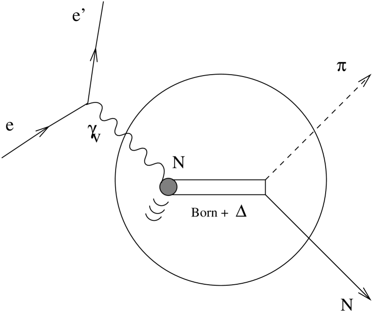
FIG. 1.: An illustration of the reaction $A(e,e^{\prime}\pi N)B$ in the $\Delta$ region.

FIG. 2.: The $k^{2}$ and W dependence of the separated total cross sections for the inclusive reaction $p(e,e^{\prime})$ is compared to the data [25]. The upper curves are for the transverse cross section $\sigma_{T}$, lower curves for longitudinal cross section $\sigma_{L}$. The solid curves are calculated in the laboratory frame, whereas the dotted curves in the c.m. frame. The triangles are the real photon points [26].

FIG. 3.: The separated longitudinal and transverse differential cross sections of the reaction $p(e,e^{\prime}\pi^{+})n$ are plotted as function of the virtual photon four-momentum squared $k^{2}$ at $\theta_{\pi}=0$ and W=1175 MeV. The data points are from Saclay [27] and Bonn [28].

FIG. 4.: Separated cross sections $d\sigma_{\scriptscriptstyle T}/d\Omega_{\pi}+\epsilon\,d\sigma_{\scriptscriptstyle L}/d\Omega_{\pi}$ as a function of W at fixed $k^{2}$ and $\theta_{\pi}$. The solid lines are calculated with the full operator; dotted lines with the same form factors and no gauge fixing terms; dashed lines with the quadrupole component left out. Data are from Ref. [28].

FIG. 5.: Same as in Fig. 4, but for the interference cross section $d\sigma_{\scriptscriptstyle TL}/d\Omega_{\pi}$.

FIG. 6.: Pion azimuthal angular dependence of the virtual photoproduction cross sections are compared with the data [28] at $k^{2}=-0.15\;(GeV/c)^{2}$, W=1160, 1200 MeV and $\theta_{\pi}=15^{0},\;25^{0},\;35^{0}$. The legends are the same as in Fig. 4.

FIG. 7.: The $\theta_{\pi}$ distributions for the virtual cross section of $p(e,e^{\prime}\pi^{0})p$ are compared to the data from Bonn [29] for two pion azimuthal angles. The solid lines are calculated with the full operator; dotted lines with the same form factors and no gauge fixing terms; dashed lines without the quadrupole component.

FIG. 8.: Polarization cross section $d\sigma_{\scriptscriptstyle TT}/d\Omega_{\pi}$ as a function of W at $k^{2}=-1\;(GeV/c)^{2}$ and 4 values of $\theta_{\pi}$. The solid lines are calculated with the full operator; dotted lines with the same form factors and no gauge fixing terms; dashed lines without the quadrupole component. Data are from Ref. [28].

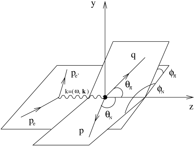
FIG. 9.: The coordinate system of the reaction $A(e,e^{\prime}\pi N)B$ in the laboratory frame.

FIG. 10.: Kinematic variables as a function of the pion angle for one case of Kinematics I. The scale for angles is on the left side and the scale for energies is on the right side. The specified variables are: $\omega$=400 MeV, $\epsilon$=0.95, $k^{2}=-0.15(GeV/c)^{2}$, $\phi_{\pi}=0$, $\phi_{p}=180^{0}$, $Q$=100 MeV/c and $\theta_{\pi}$.

FIG. 11.: Pion angular distributions of the virtual differential cross sections for $\pi^{-}$ electroproduction from ${}^{12}C$ are plotted under kinematics I, along with the contributions from the background and the resonant terms in the production operator. The kinematics and the legends to the curves are given in the figure.

FIG. 12.: Sensitivities to the quadrupole component of the $\Delta$ excitation for $\pi^{0}$ electroproduction under kinematics I.

FIG. 13.: $k^{2}$ dependence of the cross sections under kinematics I. Also shown are the sensitivities to different choice of form factors.

FIG. 14.: Distortion effects due to final state interactions of the pion and the nucleon with the residual nucleus under kinematics I.

FIG. 15.: Pion angular distribution of the differential cross sections under kinematics II are plotted along with the contributions from the background and the resonant terms in the production process.

FIG. 16.: Sensitivities to the quadrupole component of the $\Delta$ excitation for $\pi^{0}$ electroproduction under kinematics II.

FIG. 17.: Pion angular distribution of the differential cross sections under kinematics III are plotted along with the contributions from the background and the resonant terms in the production process.

FIG. 18.: Sensitivities to the quadrupole component of the $\Delta$ excitation for $\pi^{0}$ electroproduction under kinematics III.

FIG. 19.: $k^{2}$ dependence of the longitudinal and transverse cross sections in the direction of the virtual photon is shown under kinematics III along with sensitivities to the form factors. The full curve is with realistic form factors, the short-dashed curve is with dipole pion form factor instead of monopole, the long-dashed curve is with all form factors equal to $F(k^{2})=1/[1+(-k^{2})/0.71]^{2}$, and the dot-dashed curve is with no form factors.

FIG. 20.: Out-of-plane distributions of the differential cross sections are shown as a function of the average azimuthal angle $\phi=(\phi_{\pi}+\phi_{p})/2$ at fixed $\Delta\phi=\phi_{\pi}-\phi_{p}=135^{0}$ using kinematics III. Also shown are the sensitivities to the quadruple moment.

FIG. 21.: Same as in Fig. 20, but at fixed $\Delta\phi=\phi_{\pi}-\phi_{p}=180^{0}$.

FIG. 22.: The $\theta_{\pi}$ dependence of the calculated cross sections of the reaction $CO(e,e^{\prime}\pi^{-}p)$ are compared with the data from SLAC [9]. The dashed curve is the integrated PWIA result carried out according to Eq. (45). The solid curve is the DWIA result calculated according to the approximation given by Eq. (46).