Solution of the Nuclear Shell Model by
Symmetry-Dictated Truncation

The dynamical symmetries of the Fermion Dynamical Symmetry Model are used as a principle of truncation for the spherical shell model. Utilizing the usual principle of energy-dictated truncation to select a valence space, and symmetry-dictated truncation to select a collective subspace of that valence space, we are able to reduce the full shell model space to one of manageable dimensions with modern supercomputers, even for the heaviest nuclei. The resulting shell model then consists of diagonalizing an effective Hamiltonian within the restricted subspace. This theory is not confined to any symmetry limits, and represents a full solution of the original shell model if the appropriate effective interaction of the truncated space can be determined. As a first step in constructing that interaction, we present an empirical determination of its matrix elements for the collective subspace with no broken pairs in a representative set of nuclei with $130\leq A\leq 250$. We demonstrate that this effective interaction can be parameterized in terms of a few quantities varying slowly with particle number, and is capable of describing a broad range of low-energy observables for these nuclei. Finally we give a brief discussion of extending these methods to include a single broken collective pair.

1 Introduction

The shell model is fundamental to the understanding of nuclear structure, but it cannot be used for practical calculations in systems with many valence particles outside closed shells. There are two basic reasons for this. (1) The matrix dimensionalities are too large. (2) There are too many effective interaction parameters. The first problem is well known; the second is as important, but is less appreciated. We may illustrate this second problem by noting that if one views the effective interaction for a major shell of neutrons and of protons as specified by a set of matrix elements to be determined by fits to existing data, for the heaviest nuclei we must determine a minimum of about 2500 parameters (matrix elements of allowed one and two-body interactions) from some combination of theory and data. By comparison, the same approach in the $sd$ shell requires almost two orders of magnitude fewer parameters.

2 Symmetry as a Truncation Principle

This proliferation of parameters is not a failure of the theory. The large number of parameters just reflects the number of independent one and two-body scatterings that are possible within a large valence space populated by significant numbers of nucleons. Of course in all practical calculations, the number of parameters has been reduced by some means. The most drastic prescriptions are the mean field ones that replace these parameters by an average potential, and an additional set of prescriptions (often in the form of semi-empirical recipes) that prescribe how to calculate observable quantities, and how to correct at some level (again often semiempirical) for the correlations neglected in such an approximation.

The applicability of mean field theories in a variety of applications is well established, but the nuclear many-body problem cannot be reduced to mean field terms, and the semiempirical nature of mean field successes argues for a more microscopic understanding. On the other hand, the success of mean field methods, and the relative simplicity of much of low-lying nuclear structure, suggest that most of the possible contributions to the effective interaction either are negligible, or more likely, they enter (low energy) nuclear structure only in certain restricted combinations.

2.1 Modern Approaches to the Shell Model Problem

Thus, the solution of the general shell model problem for heavy nuclei requires a resolution of the matrix dimensionality problem and a consistent method to select a highly restricted subset of the effective interaction parameters as the ones relevant for low energy structure. Ideally, one would like an approach that accomplishes both of these tasks in a self-consistent manner. Traditionally one begins with some form of energy-dictated truncation. This helps with the matrix dimensionality problem by restricting the size of the shell model space, and at the same time limits the number of parameters that must be determined. However, energy-dictated truncations have had limited success for nuclei far removed from closed shells: the influence of any single high-lying configuration may be negligible, but the aggregate contribution of many such configurations may not be. Thus, energy-dictated truncations alone are unlikely to allow us to solve the general shell model problem for heavy nuclei.

There are four modern approaches to this problem of trying to extend the shell model to the description of heavy nuclei far removed from closed shells.

1. Improved algorithms and computers for traditional shell models (e. g., Refs. [1, 2, 3]).

2. Path integral solutions of the shell model using Monte Carlo algorithms on fast supercomputers (e. g., Refs. [4, 5]).

3. Truncations of the shell model space based on guidance from mean-field geometrical models with approximate pairing (e. g., Refs. [6, 7]).

4. Symmetry-dictated truncations of the shell model space (e. g., Refs. [8, 9, 10, 11]).

Approaches (1) and (2) have had some success with the matrix dimensionality problem, either by attacking it more efficiently, or by avoiding it altogether in the path integral approach. However, neither offers an intrinsic solution to the burgeoning number of effective interaction parameters in the heavy nuclei. One still must supplement these approaches with a prescription for selecting the components of the interaction that are to be emphasized. We will not address methods (1) or (2) in this review, and refer the reader to the literature cited above on these subjects [1, 2, 3, 4, 5].

On the other hand, approaches (3) and (4) help with both aspects of the problem: the truncations implied by these prescriptions reduce the matrix dimensionality, and the nature of the truncation suggests a prescription for choosing the form of the most important interaction terms in the resulting trunctated space. An excellent example of approach (3) is the Projected Shell Model [12, 7], which truncates the space using a deformed mean field plus BCS pairing prescription, and then diagonalizes a Hamiltonian composed of low-order pairing and multipole terms in the truncated basis. The approaches in category (3) have had considerable success in practical calculations, but we will not deal with them in this review, except to remark that they have many deep similarities with the symmetry-based approaches that we shall discuss.

We focus the remainder of our discussion on symmetry-dictated truncation and its integrated solution to the shell model problem: (1) the symmetries dictate a severe truncation of the shell model space; (2) the requirement that the dominant interactions respect these symmetries provides a methodology for emphasizing a limited subset of interactions. Whether such an integrated approach is useful depends on the ability of the resulting theory to describe a broad range of nuclear structure data with a restricted set of parameters that vary in a well-conditioned manner with particle number.

2.2 Symmetry-Dictated Truncation

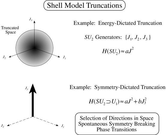
Figure 1: An illustration of energy-dictated and symmetry-dictated truncations for a simple symmetry.

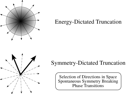
Figure 2: Energy-dictated and Symmetry-dictated truncations for a spherical shell model.

Symmetry-dictated truncation is illustrated for a simple model assuming an $SU_{2}$ symmetry in Fig. 1, and for a shell model dynamical symmetry in Fig. 2. Stated somewhat loosely, an energy-dictated truncation truncates the space “spherically” in the space of symmetry generators (for example, the three angular momentum components in Fig. 1), but a symmetry-dictated truncation reduces the space further by selecting a particular “direction” (or set of directions) in the space of symmetry generators. Representative directions are indicated schematically in Fig. 1 and Fig. 2 by the heavy arrows. Such an approach is closely associated with spontaneous symmetry breaking and phase transitions because of the selection of preferred directions in the space.

2.3 Shell Model Effective Interactions

Shell model effective interactions are highly dependent on the truncation scheme [13, 14, 15]. A realistic initial approach to obtaining an effective interaction is to treat its matrix elements as parameters to be determined from data[16]. The prototype of this method is the determination of the Brown and Wildenthal matrix elements for light nuclei [17, 18], but a literal transcription of the empirical $sd$ shell approach to the actinide nuclei would require approximately 2500 matrix elements of the effective interaction to be determined from the data.

On the other hand, in the actinide region the most general $Sp_{6}^{\nu}\times Sp_{6}^{\pi}$ Hamiltonian of the Fermion Dynamical Symmetry Model [8] requires (at most) about 100 effective interaction parameters to be determined, which is comparable to the number required in the full shell model for the $sd$ shell [17]. In reality, the symmetry-dictated truncation of the FDSM will limit the number of relevant parameters even more severely than these formal estimates would suggest: the results to be presented here indicate that most low-lying nuclear properties are determined by only of order 10 symmetry-selected parameters for the entire shell, with (at most) a weak dependence of these parameters on particle number.

2.4 FDSM Effective Interactions

Thus, the FDSM symmetry-dictated truncation provides a methodology with the potential to enable shell model calculations for all nuclei. To establish its validity, it is necessary to demonstrate through a detailed set of calculations that the required effective interaction (1) is easily determined, and (2) produces a quantitative description of observables in heavy nuclei. This will be an iterative process requiring a long series of systematic calculations, but we offer the following initial speculations concerning the FDSM effective interactions and the process of determining it:

1. The symmetry-dictated truncation of the FDSM is qualitatively different from energy-dictated truncations; it could lead to effective interactions in the highly truncated spaces that are markedly different in the components that are emphasized relative to the appropriate interactions in the full shell model space. Unlike energy-dictated truncations, a symmetry-dictated truncation selects particular “directions” in the shell model space (see Fig. 2).

2. A complicated particle number dependence for the effective interaction would make the theory difficult to use in a consistent microscopic way. Therefore, we require that the effective interaction have a smooth and/or weak particle number dependence within a shell. Since filling different valence shells defines different phases of the theory, it is possible (but not required) that the parameters could have discontinuities between shells. Likewise, it is possible (but not required) that there may be discontinuities between parameter sets describing regions having different dynamical symmetries, since these too define different phases of the theory.

3. A reasonable first step will be to determine the effective interaction in the $SD$ collective subspace of the FDSM using symmetry-limit calculations. We may then investigate deviations from the symmetry limits within the $SD$ space, and may expect that this leads to small and smooth changes of the effective interaction parameters from the symmetry-limit values.

4. Finally, we may expand the space to include broken collective pairs. This will allow the determination of additional effective interaction parameters associated with high-spin physics that played small roles in the low-lying states. In addition, we may expect a systematic renormalization of the parameters already determined in the $SD$ subspace by virtue of enlarging the space. This renormalization under space enlargement must be well behaved if the symmetry-dictated method of truncation is to be of practical utility.

Thus an important first step in this program is to take dynamical symmetry limits as a starting point and fit to the data using an FDSM Hamiltonian with symmetry breaking terms included in lowest order perturbation around the symmetry limits. Applications of the FDSM at this level have been discussed extensively in [8]. At the next level of improvement, we may assume the most general highest symmetries and a corresponding Hamiltonian, but not restrict the calculation to the dynamical symmetry limits or to perturbation around the symmetry limits. We may hope to obtain by these approximations a qualitative agreement with experiment; this effective interaction can then be refined in subsequent calculations that include more realistic configuration mixing and enlarge the space to include broken pairs.

In this review we shall emphasize two aspects of this extension of the FDSM beyond the dynamical symmetry limits. The first is the initiation of a systematic analysis of symmetry-breaking terms in the realistic shell model Hamiltonian relative to the FDSM symmetry limit Hamiltonians. The second is a series of numerical calculations that take the theory beyond the symmetry limits and begin to establish a set of effective interaction parameters for realistic symmetry-truncated shell model calculations.

3 Examples of Truncated Valence Spaces

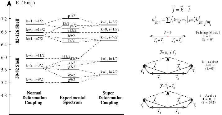
Figure 3: The FDSM coupling scheme for normal and superdeformation.

The essence of the FDSM approach is to impose a symmetry-dictated truncation within a particular valence space, with the choice of valence space often dictated by energy considerations. As has been discussed in some detail in Ref. [8], there is considerable flexibility in the choice of the space in which to implement such a truncation. The space truncation is instituted through the generalized Ginocchio [19] coupling scheme illustrated on the far right side of Fig. 3 [8]. The most common implementation has been within a single major shell, as illustrated by the coupling labeled “Normal Deformation” in Fig. 3. However, an FDSM model of superdeformation has also been proposed [20] that uses the alternative coupling scheme labeled “Super Deformation” in Fig. 3. This example makes it clear that the choice of valence space is not the central issue, but a clever choice of the valence space may enhance the ability of the symmetry limits of the theory to describe data.

More generally, it has been suggested that the FDSM can be formulated in a variety of valence spaces, with different choices associated with what would be termed shape coexistence in a mean-field theory [21]. In this review we shall concentrate on applications of symmetry-dictated truncation to major-shell valence spaces, but the basic ideas should be applicable to a broad range of valence spaces if one can implement a symmetry-dictated truncation within them. In particular, we expect that a similar analysis is possible for superdeformed states.

4 Symmetry-Breaking in the FDSM

The symmetry limits of the FDSM, and perturbation theory about those symmetry limits, describe a broad range of nuclear structure observations [8]. It is of interest to examine systematically the excursions from the symmetry limits of the theory, in order to test its suitability as a systematic truncation procedure for quantitative shell model calculations in heavy nuclei.

4.1 The Breaking of Dynamical Symmetries

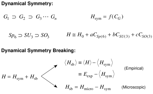
Figure 4: Dynamical symmetry and the breaking of dynamical symmetry. The Casimir invariants of the group $G$ are denoted by $C_{G}$.

Principles of dynamical symmetry and dynamical symmetry breaking are summarized in Fig. 4. A dynamical symmetry results when a Hamiltonian can be expressed in terms of invariants for the highest group and subgroups of a group chain, as we illustrate for the $Sp_{6}\supset SU_{3}\supset SO_{3}$ dynamical symmetry of the FDSM. Symmetry-breaking then corresponds to the presence of Hamiltonian terms that cannot be expressed in this manner. Figure 4 also distinguishes two approaches to dynamical symmetry breaking. The first is empirical: one defines the symmetry breaking to be the difference between the observation and the symmetry-limit calculation. This provides a definition of symmetry breaking, but is not predictive. More useful are the microscopic approaches to symmetry breaking, where the symmetry-limit Hamiltonian $H_{\mbox{\scriptsize sym}}$ is presumed to derive from a more fundamental Hamiltonian $H_{\mbox{\scriptsize micro}}$ with a known form. Therefore, one can use theoretical and physical arguments to identify likely symmetry breaking terms $H_{\mbox{\scriptsize sb}}$, and can make predictive estimates for the expected magnitude of symmetry breaking. The situation addressed here falls in this second category: the FDSM symmetry-limit Hamiltonian represents an approximation to the full shell model Hamiltonian that omits terms breaking a particular dynamical symmetry. Since the forms of the two Hamiltonians are known, we may use physical arguments to identify the terms of the full Hamiltonian that break the symmetry and are likely to be important. We now illustrate using $\mbox{$S\kern-0.41702ptp_{\kern 0.29192pt6}$}\supset\mbox{$SU_{3}$}$ symmetry breaking by spherical single-particle energies in the FDSM [22].

4.2 Symmetry Breaking by Spherical Single-Particle Energies

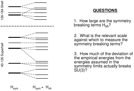
Figure 5: The difference between the symmetry-limit and realistic single-particle spectrum.

Orbitals exhibiting an $Sp(6)\supset SU(3)$ dynamical symmetry have $k=1$ (see Fig. 3). A Hamiltonian with an $Sp(6)\supset SU(3)$ dynamical symmetry requires degeneracy in the single-particle energy terms corresponding to the same value of $i$. For normal deformation in heavier nuclei, and for superdeformation, there are multiple values of $i$ within a valence shell and the symmetry-limit Hamiltonian will exhibit a higher level of degeneracy than the realistic spherical single-particle shell model spectrum (Fig. 3). The difference between the symmetry-limit and realistic spectra of Fig. 3 are shown in Fig. 5, which also summarizes several issues that are relevant to the present discussion. These concern, not simply the size of the single-particle splitting, but its size relative to the correlation energy of the system and how much of that splitting breaks the relevant symmetry [20, 8, 21].

The states of the FDSM are classified according to a total heritage quantum number $u$ that measures the number of particles not coupled to coherent $S$ and $D$ pairs [14]. Low-spin states of even–even nuclei are dominantly $u=0$ configurations. The mixing matrix elements associated with the splitting of the single-particle energies may be expressed as

$$\left<\lambda^{\prime}\mu^{\prime}u^{\prime}\left|n_{i}^{(rr)0}\right|\lambda\mu u\right>=\frac{\left<\lambda^{\prime}\mu^{\prime}u^{\prime}\left|[n_{i}^{(rr)0},C_{SU(3)}]\right|\lambda\mu u\right>}{C(\lambda\mu)-C(\lambda^{\prime}\mu^{\prime})}.$$ (1)

where $u$ and $u^{\prime}$ are the heritage quantum numbers, $C(\lambda\mu)$ is the usual eigenvalue of the quadratic $SU_{3}$ Casimir operator $C_{SU(3)}$ evaluated in an $SU_{3}$ representation $(\lambda,\mu)$, and the single-particle energy expressed in terms of the standard FDSM $k$–$i$ basis is:

$$\sum_{j}n_{j}e_{j}=\sum_{r,i}{n}^{(rr)0}_{i}e^{r}_{i},$$ (2)

where the operator ${n}^{(rr)0}_{i}$ is given by

$${n}^{(rr)0}_{i}=\sqrt{2\Omega_{i}}\left[b_{ki}^{\dagger}\tilde{b}^{\phantom{\dagger}}_{ki}\right]^{(rr)0},$$ (3)

and

$$e^{r}_{i}=\sum_{j}e_{j}\left[\begin{array}[]{ccc}k&i&j\\ k&i&j\\ r&r&0\end{array}\right]\sqrt{\Omega_{j}/\Omega_{i}}.$$ (4)

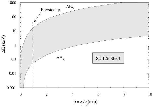
Figure 6: Range of upper limits for $SU_{3}$ symmetry breaking by single-particle energies in the 82–126 shell.

with the square bracket denoting a normalized 9-j coefficient. The $k$–$i$ basis $b_{ki}^{\dagger}$ has been defined in [19, 23, 14]; $\Omega_{j}$ and $\Omega_{i}$ are the pair degeneracies for the $j$ shell and the shells associated with pseudospin $i$, respectively [$\Omega_{j}=j+\frac{1}{2}$, and $\Omega_{i}=(2k+1)(2i+1)/2$]. Ref. [22], demonstrates that the only operator capable of mixing an $SU_{3}$ irrep in the $u=0$ bands with other $SU_{3}$ irreps is ${n}^{(11)0}_{i}$. Estimates for the upper limit on the symmetry breaking associated with this term are summarized in Fig. 6 for typical heavy, normally-deformed nuclei. A similar analysis for superdeformation suggests that the single-particle symmetry breaking associated with the FDSM model of superdeformation is even smaller than that exhibited in this example for normal deformation. Thus, we expect that spherical single-particle symmetry breaking in both normal and superdeformed nuclei will be perturbative in size for the $\mbox{$S\kern-0.41702ptp_{\kern 0.29192pt6}$}\supset\mbox{$SU_{3}$}$ symmetry of the FDSM, and the full inclusion of such terms will be unlikely to invalidate previous symmetry-limit results.

4.3 Comments on the Size of Symmetry Breaking Terms

The stability of the $SU_{3}$ dynamical symmetry for the FDSM derives from the particular structure of the Ginocchio $S$–$D$ pairs [19, 14, 8]. The single-particle terms can break the $SU_{3}$ symmetry only through an indirect Pauli effect associated with the embedding of $SU_{3}$ in the higher symmetry $Sp_{6}$. The only operator in the single-particle energy terms that can accomplish this is ${n}^{(11)0}_{i}$. In other fermion theories, such as the Elliott model [24] or the pseudo-$SU_{3}$ model [25, 26], the $SU_{3}$ symmetry is embedded in a much larger group and there are many generators that could break the symmetry directly.

This illustrates an important concept concerning symmetry breaking: the size of the symmetry-breaking terms for a particular dynamical symmetry may differ considerably from that expected based on experience with mean field theories, or even theories based on a symmetry that is formally related but implemented in a different physical manner. In this case we see that the single-particle terms have little influence on the $SU_{3}$ symmetry because of the unique properties of the pairs that generate the symmetry. On the other hand, in a deformed mean field theory one generally finds that the quantitative results are much more sensitive to the details of the initial spherical single-particle spectrum.

5 Heritage-0 Calculations for Major Shell Truncation

Let us now examine some FDSM calculations. The majority of these will employ the code FDU0 of Wu and Vallieres [27, 28] that diagonalizes the most general interaction consistent with the highest shell symmetry of the valence space. Thus, its solutions may be considered to be linear combinations of the dynamical symmetries allowed in a valence space. It is valid only for heritage-0 subspaces; thus, it is most applicable for states in even–even nuclei below angular momentum 10, where the breaking of pairs is not too important. In addition, this code assumes that $N_{1}$, the number of pairs in the normal parity orbitals of the valence shell (for neutrons or protons), is conserved. Thus, it does not incorporate directly the effects of scattering particles between the normal and abnormal parity orbitals (such effects may still be included indirectly in the effective interaction [29, 30]). Because this scattering is expected to be more important in the Pauli forbidden region lying between 1/3 and 2/3 filling of the normal parity orbitals in $S\kern-0.41702ptp_{\kern 0.29192pt6}$ shells [8, 31], the validity of FDU0 in that region is also questionable. Therefore, in this review we shall confine attention to states of low angular momentum for nuclei that do not lie in the Pauli forbidden region of $S\kern-0.41702ptp_{\kern 0.29192pt6}$ shells. For $SO_{8}$ shells, there is no such restriction and we are free to apply FDU0 calculations to all nuclei in the shell.

5.1 Hamiltonian

The most general Hamiltonian consistent with an $SO_{8}$ or $S\kern-0.41702ptp_{\kern 0.29192pt6}$ highest shell symmetry may be expressed as [27, 8]

$$H\hskip-5.0pt = \hskip-5.0pt\sum_{\sigma=\pi,\nu}\left(B_{2}^{\sigma}P^{2}_{\sigma}\kern-1.99997pt\cdot\kern-1.99997ptP^{2}_{\sigma}+B_{3}^{\sigma}P_{3}^{\sigma}\kern-1.99997pt\cdot\kern-1.99997ptP_{3}^{\sigma}+G_{0}^{\sigma}S^{\dagger}_{\sigma}S\vphantom{{}^{\dagger}}_{\sigma}+G_{2}^{\sigma}D^{\dagger}_{\sigma}D\vphantom{{}^{\dagger}}_{\sigma}\right)$$ (5)

$$+B_{2}^{\pi\nu}P_{2}^{\pi}\kern-1.99997pt\cdot\kern-1.99997ptP_{2}^{\nu}+B_{3}^{\pi\nu}P_{3}^{\pi}\kern-1.99997pt\cdot\kern-1.99997ptP_{3}^{\nu}+B_{1}^{\nu}P_{1}^{\nu}\kern-1.99997pt\cdot\kern-1.99997ptP_{1}^{\nu}+B_{1}^{\pi}P_{1}^{\pi}\kern-1.99997pt\cdot\kern-1.99997ptP_{1}^{\pi}+B_{1}^{\pi\nu}P_{1}^{\nu}\kern-1.99997pt\cdot\kern-1.99997ptP_{1}^{\pi}$$

where $S$ denotes monopole pair operators, $D$ denotes quadrupole pair operators, and $P_{r}$ denotes multipole operators of order $r$, with all quantities constructed in the $k$–$i$ truncation scheme illustrated in Fig. 3. Not all of these terms contribute for a particular highest symmetry. One finds that for spectra (which depend only on energy differences) there are at most 11 parameters for $SO_{8}^{\pi}\times SO_{8}^{\nu}$, 8 for $Sp_{6}^{\pi}\times Sp_{6}^{\nu}$, and 9 for $SO_{8}^{\pi}\times Sp_{6}^{\nu}$. In the numerical calculations that follow, we will typically use a simplified version of this Hamiltonian that retains only pairing and quadrupole terms, thereby reducing the number of free parameters to 5 or less for most cases.

5.2 Particle Number Distribution

In the calculations to be presented in this review, the number of pairs $N_{1}$ in the normal-parity levels is treated as a good quantum number and is estimated from the semi-empirical formula determined globally from the ground state spin of the odd-mass nuclei [8]:

$$N_{1}=\left\{\begin{array}[]{ll}N&~{}\mbox{for}~{}N<1.5\\ 0.75+0.5N&~{}\mbox{for}~{}1.5<N<2\Omega_{0}+1.5\\ N-\Omega_{0}&~{}\mbox{for}~{}N>2\Omega_{0}+1.5\end{array}\right.$$ (6)

where $N$ is the number of valence pairs and $\Omega_{0}$ is the pair degeneracy of the abnormal-parity level. The above formulas are suitable for both protons and neutrons, and are found to be in excellent agreement with a similar distribution obtained empirically from the Nilsson level scheme with a measured deformation parameter $\beta$.

5.3 Masses of Heavy and Superheavy Nuclei: Z=110–111

In recent years, evidence has accumulated [32, 33, 34] for extension of the known elements to larger proton number, culminating in the discovery of several isotopes having proton number $Z=110-111$ [35]. The usual view is that these isotopes represent the tail of the “normal element” distribution, and that the predicted superheavy elements represent a qualitatively different set of nuclides that remain undiscovered at a predicted proton number of about 114 and a neutron number approximately 20 units heavier than for the recently-discovered isotopes of elements 110 and 111. As we now discuss, truncated shell model calculations suggest a different interpretation of these results that could have important experimental implications [36, 37].

5.3.1 Comparison of Mass Calculations for Very Heavy Elements

In Table 1, we compare the observed mass excesses (first row, labeled “Exp”) for isotopes of the heaviest elements with calculations for these masses. A perusal of these results suggests that the FDSM mass calculations described in Ref. [36] give a global description of the heaviest elements that is arguably the best now available. This is particularly noteworthy because the FDSM calculations were not tuned specifically to these heaviest elements; the parameters employed in Ref. [36] were determined by a global fit to all available masses above $Z=82$ and $N=126$. We also emphasize that the accurate description of the $Z=110-111$ isotopes represents a pure prediction of the FDSM theory, published before their discovery, and without adjustments to the theory based on specific properties of the $Z=108-109$ elements that were known at the time of the calculations.

5.3.2 Superheavy Elements

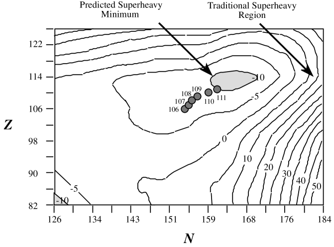
Figure 7: Mass shell correction for heavy and superheavy elements using the dynamical symmetry methods of Ref. [36].

An island of superheavy elements was found in the FDSM mass calculations [36], but this island was shifted to considerably lower neutron number than is predicted in classical calculations of the stability of superheavy elements, was found to be more stable than in such calculations, and was found to correspond to nuclei having near-spherical shapes. The shell correction associated with this minimum is illustrated in Fig. 7 for the case of a spherical Woods–Saxon single-particle spectrum. The location of the new predicted maximal shell stabilization, the traditional location of the island of superheavy stability, and the new isotopes of elements 110–111, are also shown in Fig. 7. These properties of the FDSM heavy-element solutions are consequences of two general physical principles. The first is a monopole–monopole interaction that is expected to be present on general shell-model grounds, and found from empirical mass fits to become increasingly repulsive in moving away from the stable nuclei. The second is that the structure of these heaviest elements is expected to involve a competition between an $SU_{2}$ dynamical symmetry favoring spherical symmetry and an $SU_{3}$ dynamical symmetry favoring axially symmetric deformation [8].

5.3.3 Experimental Implications

Since Ref. [36] was a general treatment of nuclear masses that was not tuned to predict the properties of these heavy new isotopes, we are emboldened to draw some general conclusions from this successful prediction that differ from those of more traditional approaches to the stability of the heavy elements [37].

1. The observation of isotopes with proton number $Z=110-111$ having the predicted properties may indicate a shift of the superheavy island of stability to considerably lower neutron numbers, as predicted in Ref. [36].

2. These new isotopes are expected to be near-spherical or deformation-soft structures, in contrast to the heavy elements with $Z\leq 106$, which are found in the FDSM (and other) calculations to have well-deformed ground states, and to most other descriptions of the new $Z=110-111$ elements, which find them to have deformed ground states.

3. The successful prediction of the masses of these new isotopes is further evidence supporting the importance of the monopole–monopole interaction introduced in [36] for the description of nuclear masses.

4. No shell stabilization minimum is expected at the traditional location of the superheavy elements because of the repulsive monopole–monopole interaction. Thus, we predict that the traditional island of superheavy elements does not exist, and that the r-process element production path may run closer to the stability valley than has generally been assumed for the heaviest elements [38].

The present hypotheses have some consequences that are testable, though the experiments are difficult. (1) There should exist nuclides of elements $Z=$ 112–114 that are approximately as stable as those of elements 110–111 (see Fig. 7). (2) Beyond $Z\simeq 116$ and $N\simeq 170$, the heavy nuclei should rapidly become less stable, and the region of traditional superheavy nuclei should be quite unstable (see Fig. 7). (3) The nuclides in this new region of superheavy nuclei ($Z\simeq 110-116$ and $N\simeq 160-170$) are expected to be either spherical or very deformation soft, with attendant consequences for properties such as the alpha decay systematics. (4) The implied shift of the r-process path closer to the stability valley should also have observable consequences, but this may require an improved understanding of the astrophysical environment for the r-process.

5.4 The Xe–Ba Region

The FDSM is defined by a fermionic Lie algebra, has symmetry limits analogous to all the IBM limits, and takes the Pauli principle into account [19, 39]. Furthermore, the states for even and odd systems in the FDSM belong to vector and spinor representations, respectively, of $SO_{8}$ or $Sp_{6}$, thus allowing a description of even–even and even–odd nuclei without the necessity of additional degrees of freedom. Therefore, symmetry-truncated shell model calculations based on the FDSM dynamical symmetries for even and odd nuclei offer a microscopic alternative to IBM and nuclear supersymmetry (NSUSY) as means to unify the structure of even and odd systems.

Nuclei in the Xe–Ba region have neutrons and protons in the 6th shell, with FDSM pseudo-orbital angular momentum $k=2$ and pseudo-spin $i=\frac{3}{2}$ for the normal-parity levels. Thus they are expected to possess $SO^{\pi}_{8}\times SO^{\nu}_{8}$ symmetry, which contains an $SO_{8}^{\pi+\nu}$ subgroup, and to have analytic solutions for $SO_{5}\times SU_{2}$, $SO_{6}$, and $SO_{7}$ dynamical symmetries. For these reasons, the Xe–Ba region is an excellent one in which to investigate a unified FDSM description of even–even and even–odd nuclei.

5.4.1 Energy Spectra

The wavefunctions for both even and odd nuclei are given by the following group chain

$$(~{}SO^{i}_{8}~{}\supset~{}SO^{i}_{6}~{}\supset~{}SO^{i}_{5}~{})\times SO^{k}_{5}~{}~{}\supset~{}SO^{i+k}_{5}~{}\supset SO^{k+i}_{3}~{}~{}~{}~{}~{}~{}~{}~{}~{}~{}~{}~{}~{}~{}~{}$$ (7)

$$~{}~{}[l_{1}l_{2}l_{3}l_{4}]\hskip 11.38092pt[\sigma_{1}\sigma_{2}\sigma_{3}]\hskip 11.38092pt[\tau_{1}\tau_{2}]\hskip 19.91684pt[\tau]\hskip 34.14322pt[\omega_{1}\omega_{2}]\hskip 22.76228ptJ~{}~{}~{}~{}~{}~{}~{}~{}~{}~{}~{}~{}~{}~{}~{}~{}~{}~{}~{}~{}~{}~{}~{}$$

where $[l_{1}l_{2}l_{3}l_{4}]$, $[\sigma_{1}\sigma_{2}\sigma_{3}]$, and $[\tau_{1}\tau_{2}]$ are the Cartan–Weyl labels for the groups $SO_{8}$, $SO_{6}$, and $SO_{5}$, respectively, $\tau=0(1)$ for even (odd) nuclei, and $k$ and $i$ indicate pseudo-orbital and pseudo-spin parts of the groups, respectively. The energies for even systems are

$$E^{\mbox{\scriptsize even}}=E^{\scriptsize\rm(e)}_{0}+g_{6}\sigma(\sigma+4)+g^{\prime}_{5}\tau(\tau+3)+g^{\prime}_{I}J(J+1),$$ (8)

and for odd systems,

$$E^{\mbox{\scriptsize odd}}= E^{\scriptsize\rm(o)}_{0}+g_{6}[\sigma_{1}(\sigma_{1}+4)+\sigma_{2}(\sigma_{2}+2)+(\sigma_{3})^{2}]+g_{J}J(J+1)$$ (9)

$$+(g^{\prime}_{5}-g_{5})[\tau_{1}(\tau_{1}+3)+\tau_{2}(\tau_{2}+1)]+g_{5}[\omega_{1}(\omega_{1}+3)+\omega_{2}(\omega_{2}+1)].$$

More details on the construction of these formulas, and the reduction rules for even and odd systems, are given in Ref. [40].

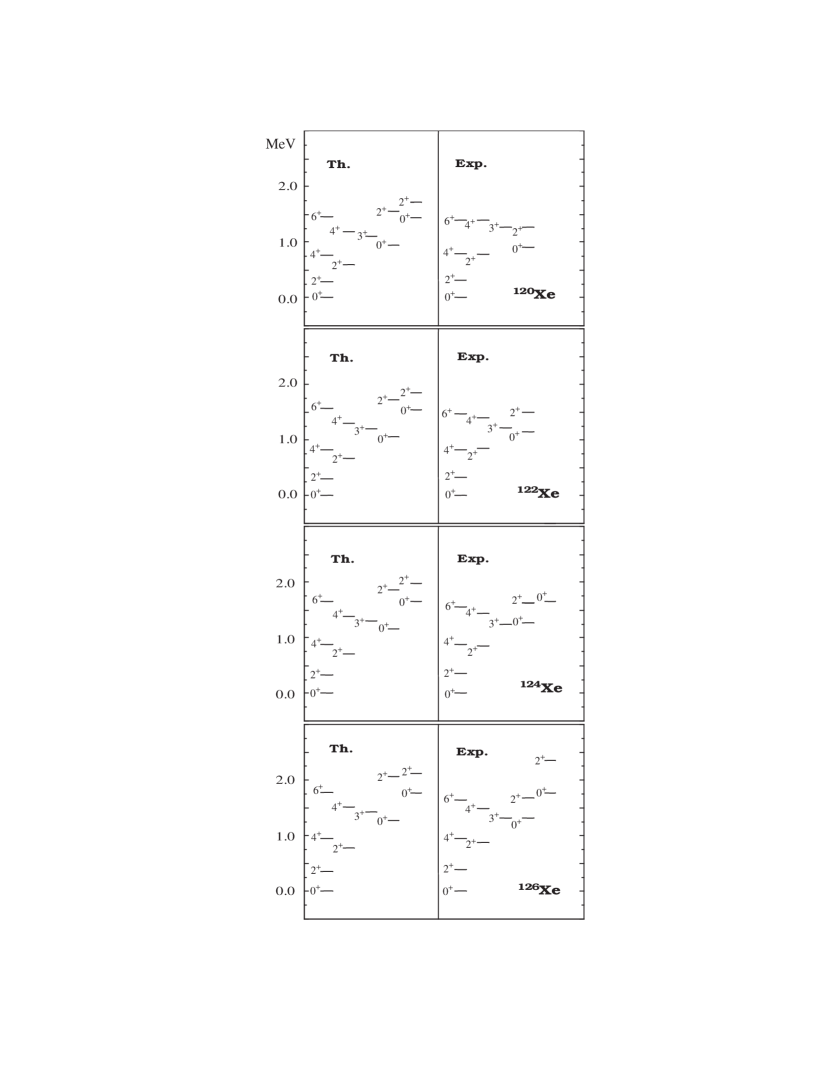
Figure 8: Comparison between calculated levels using eq. (8), and experimental energy levels for the even–even ^120-126Xe isotopes.

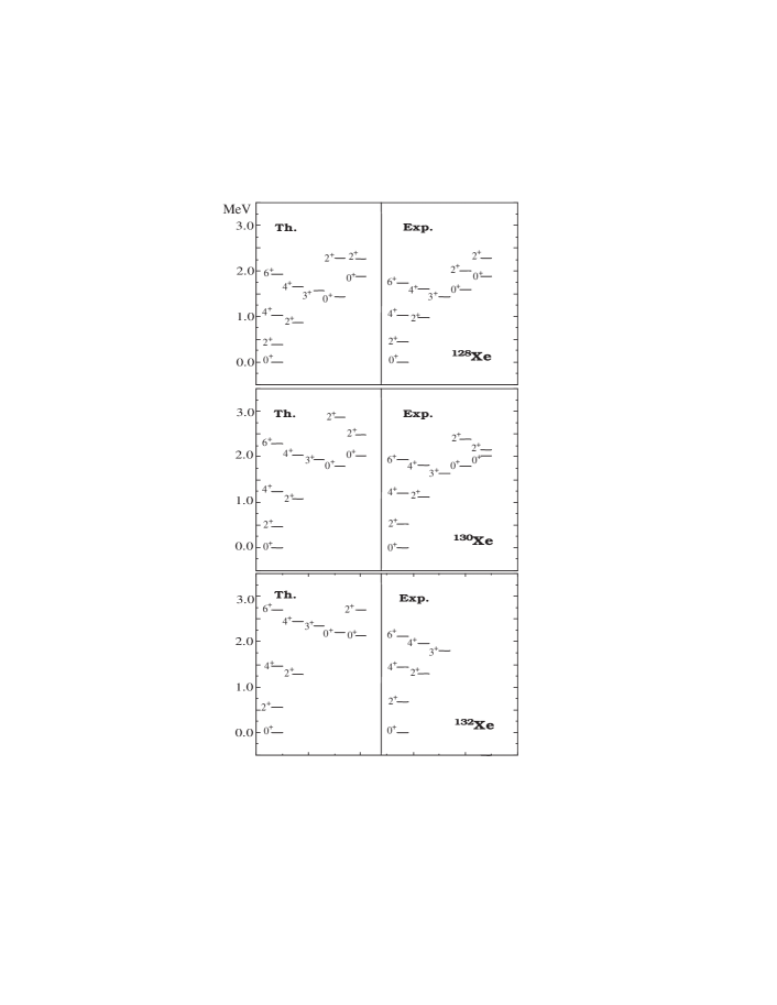
Figure 9: Comparison between calculated levels using eq. (8) and experimental energy levels for the even–even ^128-132Xe isotopes.

The low-energy spectra for ^120-132Xe isotopes predicted by Eq. (8) are compared with data in Fig. 8 and Fig. 9, and the parameters used in the calculations are given in Table 4. The experimental spectra indicate that the $SO_{3}$ parameter $g^{\prime}_{I}$ is not sensitive to the neutron number in fitting the spectra of a chain of isotopes (including both even–even and even–odd nuclei). Therefore, in fitting the even–even nuclear spectra we fix the $g^{\prime}_{I}$ parameter to be 11.9 keV and the adjustable parameters were taken to be $g_{6}$ and $g^{\prime}_{5}$.

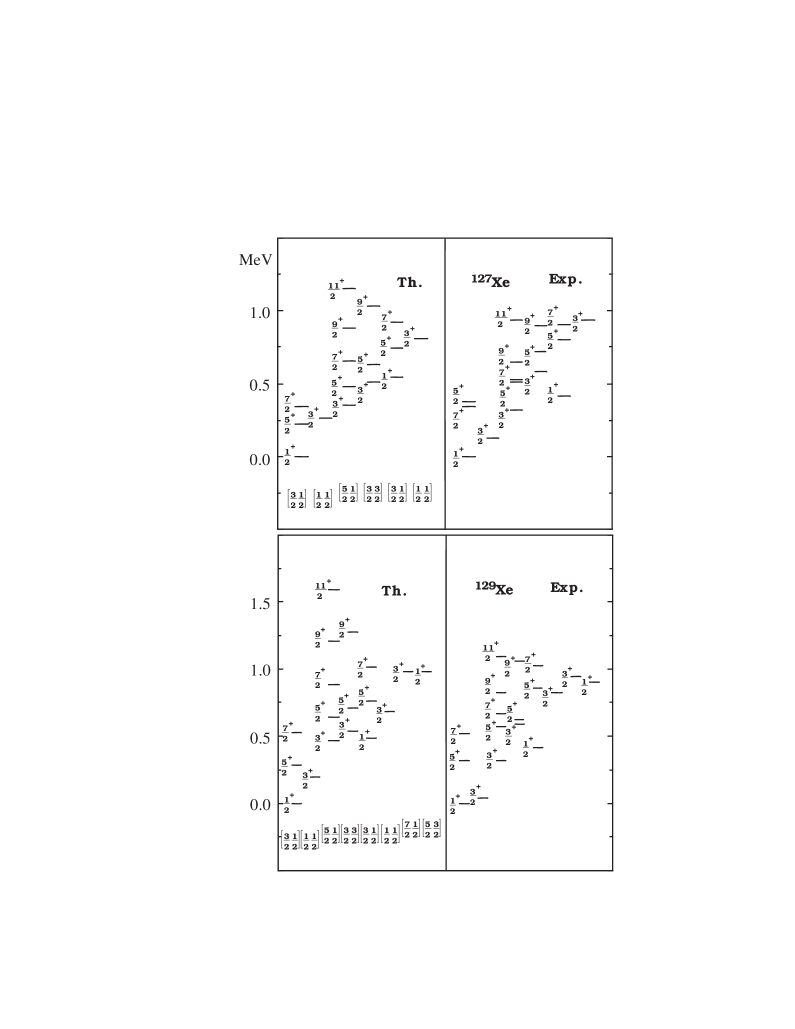
Figure 10: Comparison between calculated levels using eq. (9) and experimental energy levels for the even–odd ^127-129 Xe isotopes. The even–odd nuclei are constructed by coupling the neighboring even–even core to a valence neutron.

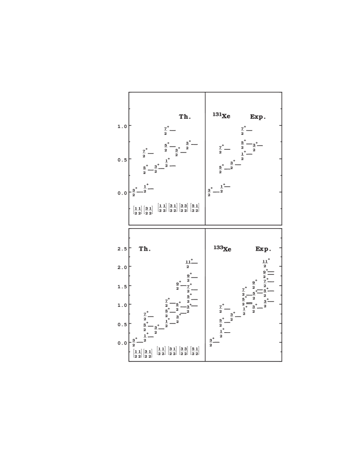
Figure 11: Comparison between calculated levels using eq. (9) and experimental energy levels for the even–odd ^131-133Xe isotopes. The even–odd nuclei are constructed by coupling the neighboring even–even core to a valence neutron.

Using Table 4 and Eq. (9), the spectra of the neighboring even–odd Xe isotopes can be calculated. We present the calculated and experimental results for ^127-133Xe in Figs. 10–11, with the parameters given in Table 4. Similar results for Ba isotopes may be found in Ref. [40]. Apart from the constant term, the formula for $E^{\mbox{\scriptsize even}}$ contains three parameters, and that for $E^{\mbox{\scriptsize odd}}$ contains two parameters beyond the three parameters that are determined by fitting the spectra of neighboring even–even nuclei. With two extra parameters, Eq. (9) reproduces the spectral patterns for the nuclei ^127-133Xe and ^131-135Ba (not shown here; see Ref. [40]) with about 15 levels each.

5.4.2 Electromagnetic Transition Rates

In Ref. [40], formulas are presented for the reduced quadrupole transition strengths $B(E2)$ in both even and odd systems. Table 5 summarizes some $B(E2)$ values calculated for even–even Xe isotopes. Similar results for Ba isotopes may be found in Ref. [40]. These are seen to agree rather well with the observations, and are indicative of a good $SO_{6}$ symmetry in this region. In Table 6, both experimental and theoretical $B(E2)$ values for the even–odd nuclei of ¹²⁹Xe and ¹³¹Xe are given, and compared with the results of NSUSY calculations. The agreement with data is comparable in the two cases.

5.4.3 Fermion Dynamical Symmetry versus Supersymmetry

In Ref. [40] it is shown that when the $u=1$ fermion $SO_{6}$ state for the FDSM core is replaced by a boson state and the Pauli factor is ignored, the FDSM wavefunction goes over to an NSUSY wavefunction. Thus, NSUSY can be obtained as an approximation to the FDSM for odd-mass $SO_{6}$ nuclei. The full FDSM without this approximation implies corrections to the NSUSY picture.

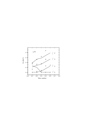
Figure 12: The systematic shift of the ground band as a function of mass number for Xe isotopes.

In the $U(6/4)$ NSUSY, the ground-state representation is $[{1\over 2}{1\over 2}]$ and the ground-state spin is always ${3\over 2}$. However, both ${1\over 2}$ and ${3\over 2}$ are observed as ground-state spins in this region. The second $SO_{5}$ Casimir operator in Eq. (9) allows this possibility: for alternative signs of the parameter $g_{5}$, the ground state spin can take the values ${1\over 2}$ or ${3\over 2}$ . What is more, by allowing $g_{5}$ to change smoothly from positive to negative, the systematic shift of the ground band for the Xe (and Ba) isotopes can be reproduced, as shown for Xe in Fig. 12.

The general conclusion of Ref. [40] is that the FDSM symmetry-dictated solution in the mass-130 region provides a unified description of even and odd nuclei that is comparable to, or better than, IBM and NSUSY approaches, but with a firmer microscopic basis. As one example of this microscopic basis, the group chain corresponding to odd-mass $SO_{6}$ nuclei in the FDSM is very similar to the corresponding NSUSY group chain, but pseudo-orbital angular momentum 2 is an ad hoc introduction in the NSUSY, while in the FDSM it is a natural result of the $k$–$i$ reclassification for the shell model single-particle states in the sixth major shell.

5.4.4 Tau Compression

Pure $SO_{6}$ spectra give reasonable agreement with data for $\tau\leq 3$ states in ^120-126Xe (see Figs. 8–9). However, the experimental energies for the higher $\tau$ values in ^128-132Xe are lower than predicted, with the discrepancies increasing with increasing $\tau$. Energy levels within the same $SO_{5}$ irrep (same $\tau$) follow the $J(J+1)$ rule rather well, so this discrepancy cannot be caused by the usual stretching effect. In Ref. [41], it was shown that this is an $SO_{5}$ $\tau$-compression effect whose driving force is the reduction of pairing correlation with increasing $\tau$. Allowing for $g_{S}=G_{0}-G_{2}\not=0$, thereby deviating from the $SO_{6}$ limit, and treating the $g_{s}S^{\dagger}\cdot S$ term as a perturbation leads to the following energy formula,

$$E^{\prime}_{\mbox{\scriptsize even}}\cong E^{\scriptsize\rm(e)}_{0}+g_{6}\sigma(\sigma+4)+A^{\prime}\tau(\tau+3)-B^{\prime}[\tau(\tau+3)]^{2}+g^{\prime}_{I}J(J+1).$$ (10)

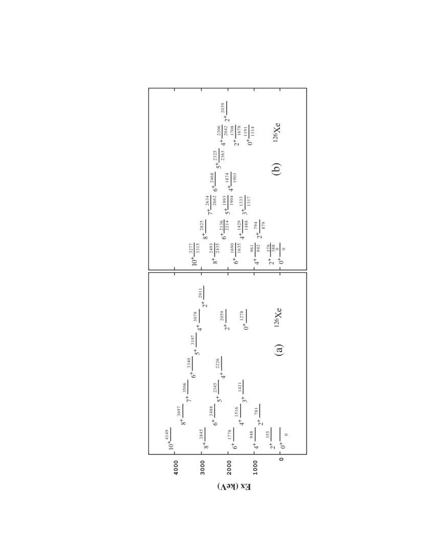
Figure 13: The tau compression effect: (a) calculated with Eq. (8) and (b) with Eq. (10). Theoretical energy is shown above and experimental energy below each level.

Fig. 13 shows the spectrum for ¹²⁶Xe predicted by Eqns. (8) and (10), respectively. Inclusion of the $SO_{5}$ stretching effect improves the agreement with data significantly. Details and more examples may be found in Ref. [41].

5.5 SO(6)-Like Behavior in the Pt Region

Numerical studies using the FDSM have shown that there is an effective $SO(6)$ fermion dynamical symmetry in the ¹⁹⁶Pt mass region [42, 43]. More recently, a systematic description of nuclear structure has been given in this region using symmetry-truncated shell model methods [43]. In this section, we review these calculations for the platinum isotopes and the emergence of effective $SO(6)$-like behavior from numerical calculations near ¹⁹⁶Pt, where the FDSM has no formal $SO_{6}$ symmetry.

5.5.1 Hamiltonian and Spectra

The five-parameter Hamiltonian is taken to be

$$H=G^{\prime}_{0\pi}S^{{\dagger}}_{\pi}S_{\pi}^{\phantom{{\dagger}}}+G^{\prime}_{0\nu}S^{{\dagger}}_{\nu}S_{\nu}^{\phantom{{\dagger}}}+B^{\prime}_{2\pi}P^{2}_{\pi}\cdot P^{2}_{\pi}+B^{\prime}_{2\nu}P^{2}_{\nu}\cdot P^{2}_{\nu}+B_{2\pi\nu}P^{2}_{\pi}\cdot P^{2}_{\nu}.$$ (11)

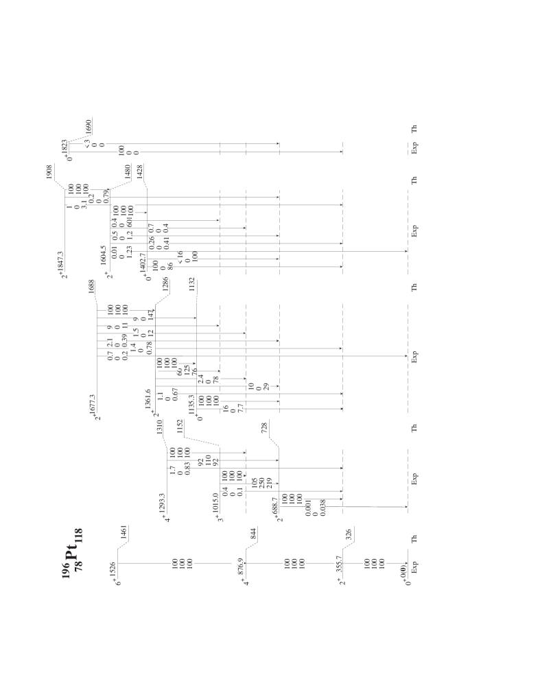
Figure 14: Level scheme for positive-parity states in ¹⁹⁶Pt. Experimental levels are taken from [57].

In the $SO(8)$ and $Sp(6)$ algebras, the quadrupole pairing interaction in this Hamiltonian is not independent and can be accounted for by redefining the parameters $G^{\prime}_{0\sigma}=G_{0\sigma}-G_{2\sigma}$ and $B^{\prime}_{r\sigma}=B_{r\sigma}-G_{2\sigma}$ ($\sigma=\pi,\nu$). The spectra of five even platinum isotopes ^190-198Pt (there are approximately 13 levels for each nucleus) are found to be satisfactorily described by sets of five parameters. In Figs. 14 and 15 the calculated spectra for ^190-198Pt are compared with the data; the corresponding parameters are summarized in Table 7.

Fig. 15 indicates that most low-lying $0^{+}$ and $2^{+}$ states are well reproduced by the FDSM calculations, tolerable agreement is obtained for the $4^{+}$ states, and there is a persistent deviation of the calculated $3^{+}$ states that increases with mass. The basic theoretical trends are the narrowing of the energy gap between the $3^{+}_{1}$ and $4^{+}_{1}$ levels, and a widening of the gap between the $3^{+}_{1}$ and $2^{+}_{2}$ levels. This level pattern is characteristic of the $SO_{6}$ dynamical symmetry and appears naturally in the heavier Pt isotopes. In Fig. 14, we have presented a separate spectrum for ¹⁹⁶Pt, in order to show the experimental $E2$ branching ratios as well as the corresponding FDSM and IBM–2 predictions. The overall FDSM results are in quantitative agreement with the $O(6)$ level pattern and the $SO_{6}$ $E2$ selection rules in the FDSM description of ¹⁹⁶Pt. This agreement confirms that the FDSM does not have an explicit mathematical $SO(6)$ dynamical symmetry for this case, but it has a remarkably accurate practical one [42].

5.5.2 Electromagnetic Transitions

The FDSM wavefunctions obtained through the diagonalization of the Hamiltonian can be used to compute multipole transition strengths. Expressions for quadrupole moments and $B(E2)$ values, dipole moments and g-factors, and isomer and isotope shifts may be found in Ref. [43]. In Table 8, we have compiled the experimental $B(E2)$ values and predictions from the FDSM and various versions of the IBM for ¹⁹⁶Pt. Additional comparisons for the other isotopes of Pt may be found in Ref. [43]. Also shown in the ¹⁹⁶Pt table are $SO_{6}$ limit results. (IBM–1(g) means IBM–1 with one g-boson explicitly included and the effective charge individually fitted from nucleus to nucleus; in the IBM–2 calculation the effective charge remains constant for all the platinums, just as for the FDSM calculations.) Table 9 compares experimental g-factors with FDSM and IBM calculations, and calculated isomer and isotope shifts are compared with data in Table 10.

5.5.3 F-Spin and Majorana Interactions

In boson-model calculations, $F$-spin is used to distinguish low-lying symmetric and mixed symmetry states [44], and a “Majorana interaction” is typically introduced to guarantee that mixed symmetry states do not appear at unacceptably low energies. For fermions there is no closed $F$-spin algebra and no explicit Majorana interaction in the Hamiltonian: for a fermion many-body system, the relative positions of the symmetric and mixed-symmetry states are governed by the basic pairing and multipole interaction strengths. For the ¹⁹⁶Pt case that we discuss, the mixed-symmetry $1^{+}$ state is at an excitation energy of approximately 2 MeV, and is correctly predicted without introducing the analog of a Majorana term. Thus, the effective fermion $SO(6)$ symmetry produces a quantitative agreement with the spectrum using a simpler Hamiltonian than is required in the IBM–2.

5.6 Effective Interaction for Rare Earth Nuclei

The parameters used in reproducing the $SO(6)$-like spectrum and the branching ratios of the platinum isotopes do not represent a peculiar set chosen solely for this purpose. Similar calculations in the remainder of the rare earth nuclei indicate that the Pt parameters are related to the effective interactions of the entire shell. For example, if the same five parameters are used in the FDU0 calculation but the appropriate valence particle numbers for heavy Gd isotopes are chosen, the spectrum and transition rates become $SU(3)$-like (axially-symmetric rotors). With only small adjustments in these parameters (for example, less than 5% for the n–p quadrupole coupling, which is the dominant parameter) the spectrum and transition rates for the low-lying states in the heavier Gd isotopes can be quantitatively reproduced. Likewise, a similar set of parameters leads to vibrational ($SU(2)$-like) spectra for valence particle numbers near the beginning or the end of the shell.

These results imply that a fixed Hamiltonian with parameters varying slowly with particle number can produce spectra that evolve from $SU(2)$ to $SU(3)$, from $SU(3)$ to $SO(6)$, and from $SO(6)$ to $SU(2)$, as the proton or neutron number changes. This $SU(2)$–$SO(6)$–$SU(3)$ triangle is similar to the $SU(5)$–$O(6)$–$SU(3)$ triangle relation [45] of the IBM. However, unlike the IBM, the triangle relationships in the FDSM are shell dependent. For the $SO(8)\times SO(8)$ shells, there is no $SU(3)$ limit and the $SO(6)$ symmetry is the most collective limit (corresponding to $\gamma$-unstable rotations). In this case the triangle relationship is replaced by $SU(2)$–$SO(7)$–$SO(6)$. We have speculated [42] that whenever there is a vibrational ($SU(2)-$like) symmetry limit on one corner of the triangle and an $SU(3)-$like rotational limit on a second corner of the triangle, an $SO(6)$-like effective transitional symmetry may occur, even though there is formally no such dynamical symmetry in these shells.

5.7 Universality of Normal and Exotic States

The measured electromagnetic transition strengths $B(E2)$ between the ground states and first $2^{+}$ states of even–even rare earth nuclei vary with mass number $A$ in a way quite similar to that of the summed orbital $B(M1)$ strengths measured in the same nuclei [46]. The observed correlation in these strengths suggests a microscopic relationship between modes that are qualitatively different in the simplest geometrical picture. Assuming that all $M1$ strength has been detected experimentally, it is difficult to explain simply within the IBM $F$-spin symmetry the observation that both the $E2$ and $M1$ strengths saturate well before midshell [47]. The FDSM is known to reduce to an IBM model in the limit of neglected Pauli correlations [8], so it is reasonable to ask whether a model such as the FDSM that incorporates the fermionic nature of the correlated pairs can account for the similar behavior of $E2$ and $M1$ strengths.

As noted in the preceding section, the $F$-spin algebra of IBM–2 allows the introduction of an $F$-spin scalar (the Majorana interaction) that is insensitive to the normal symmetric states. Thus, It may be chosen to have a strength that pushes the mixed-symmetry states to their proper energies. Unlike the IBM–2, the FDSM cannot have a closed $F$-spin algebra. Thus, one is compelled to describe all states, symmetric or mixed-symmetry, in terms of a single Hamiltonian whose eigenstates must reflect the subtle balance between n–p quadrupole interactions and the n–n and p–p pairing forces.

5.7.1 Hamiltonian and Operators

We employ a 5-parameter (pairing and QQ) FDSM Hamiltonian:

$$H=G^{\prime}_{0\pi}S^{{\dagger}}_{\pi}S_{\pi}^{\phantom{{\dagger}}}+G^{\prime}_{0\nu}S^{{\dagger}}_{\nu}S_{\nu}^{\phantom{{\dagger}}}+B^{\prime}_{2\pi}P^{2}_{\pi}\cdot P^{2}_{\pi}+B^{\prime}_{2\nu}P^{2}_{\nu}\cdot P^{2}_{\nu}+B_{2\pi\nu}P^{2}_{\pi}\cdot P^{2}_{\nu}.$$ (12)

The operators are defined in [8] and the FDSM quadrupole pairing interaction is taken into account by renormalizing the parameters: $G^{\prime}_{0\sigma}=G_{0\sigma}-G_{2\sigma}$ and $B^{\prime}_{r\sigma}=B_{r\sigma}-G_{2\sigma}$ ($\sigma=\pi,\nu$). The five parameters in Eq. (12) were determined numerically using a gradient search with the FDU0 code [27, 28] fitted to the experimental energies of the available $2^{+}_{1}$, $4^{+}_{1}$, $6^{+}_{1}$, $1^{+}$, $2^{+}_{2}$, and $0^{+}_{2}$ states in Nd, Sm, Gd, Dy, and Er. These calculations indicate that the QQ-interaction plays the crucial role in correlating the energies of the $2^{+}_{1}$ and $1^{+}$ states. Using these parameters, we may then ask whether there is a correlation between symmetric and mixed-symmetry states caused by the same $Q_{\pi}\cdot Q_{\nu}$ strength for the electromagnetic transitions.

5.7.2 Spectrum and Multipole Strengths

In Fig. 16 the experimental and calculated energies of the $2^{+}_{1}$ and $1^{+}_{1}$ state energies are plotted versus the $P$ factor [48, 46], $P\equiv N_{p}N_{n}/(N_{p}+N_{n})$, where $N_{p}$ ($N_{n}$) are the valence proton (neutron) numbers, respectively. The $B(E2)$ values and the summed $B(M1)$ strengths resulting from this calculation are compared with measured quantities in Fig. 17. The curves are the empirical relations presented in [46] that summarize the approximate behavior of the data. The $B(E2)$ and $B(M1)$ strengths are reproduced quantitively by the calculations (with the single exception of the ¹⁶⁴Dy point). Thus, we find theoretical evidence for the approximate universal behavior of $E2$ and $M1$ strengths exhibited by the data. Furthermore, even the deviations from universality exhibited by the data are reproduced by the calculations without parameter adjustment. In Figs. 17c and 17c^′, we have plotted the ratio $E(4^{+}_{1})/E(2^{+}_{1})$ as a function of $P$. This quantity also varies with $P$ in a way similar to that of the $E2$ and $M1$ strengths, and is also quantitively reproduced by these calculations.

Finally, we address the question of how important the variation of effective interaction parameters is to the success of the calculations we have described. In Figs. 17a^′′–c^′′ we repeat the calculations of Figs. 17a^′–c^′, but with a fixed set of parameters for all nuclei: $G^{\prime}_{0\pi}=-0.074$ MeV, $G^{\prime}_{0\nu}=0.020$ MeV, $B^{\prime}_{2\pi}=-0.001$ MeV, $B^{\prime}_{2\nu}=0.047$ MeV, and $B_{2\pi\nu}=-0.243$ MeV. The results of this calculation are seen to differ in minor details only from the previous calculations in which the effective interaction was permitted to have a weak $A$ dependence. Thus, the quantitative reproduction of $E2$ and $M1$ strengths in the rare earth nuclei is an inherent feature of the FDSM with a constant effective interaction.

6 Higher Heritage Configurations

The FDSM is a truncated shell model with symmetry-dictated $S$ and $D$ pairs. In its simplest implementation, one restricts the space to heritage $u=0$; then all nucleons form $S$ or $D$ fermion pairs:

$$A^{\dagger r}_{\mu}=\left\{\begin{array}[]{ll}\sqrt{\Omega_{1}/2}\left[b^{\dagger}_{ki}b^{\dagger}_{ki}\right]^{0r}_{0\mu},~{}~{}~{}r=0,\,2&~{}\mbox{for i-active}\\ &\\ \sqrt{\Omega_{1}/2}\left[b^{\dagger}_{ki}b^{\dagger}_{ki}\right]^{r0}_{\mu 0},~{}~{}~{}r=0,\,2&~{}\mbox{for k-active}\end{array}\right.~{}~{},$$ (13)

where $i=\frac{3}{2}$ or $k=1$, $S^{\dagger}=A^{\dagger 0}$ and $D^{\dagger}_{\mu}=A^{\dagger 2}_{\mu}$, and $\Omega_{1}$ is the degeneracy for the normal-parity levels of a major shell.

As we have seen, this space gives a good description for even–even nuclei in states of low angular momentum. However, numerical calculations within the $u=0$ space consistently overestimate the energies and underestimate the $B(E2)$ values for higher angular momentum states, and these discrepancies increase with angular momentum. Some improvement can be gained in the energies by correcting perturbatively for the influence of pairing in the same manner as the $SO(5)$ + pairing approach discussed previously. However, it has been realized since the inception of the FDSM that the primary reason for these discrepancies is the significant contribution of broken pairs to high angular momentum states [49, 50]. Broken pairs in normal or abnormal parity orbitals may carry significant angular momentum, thereby reducing the amount carried by the $S$–$D$ condensate. As was demonstrated schematically in Refs. [49, 50], this leads to a Variable Moment of Inertia (VMI) behavior for the moment of inertia similar to that observed experimentally, and brings calculated and observed high-spin $B(E2)$ values into quantitative agreement with data [50, 51, 8].

Thus, it is natural to extend the numerical implementation of symmetry dictated truncation by using the FDSM to include unpaired particles. This has been discussed for a single unpaired particle in Refs. [52, 53, 54, 8]. We shall not discuss that further here, but instead conclude by summarizing recent work that incorporates broken pairs in such calculations. We have developed a computer code SU3su2 that includes explicit broken pairs in an $SU(3)$ limit in order to examine the yrast states in the rare earth and actinide regions [55, 56]. In this extension, the model basis is constructed by coupling the $SU(3)$ basis and one broken pair in the normal parity levels or the unique parity level

$$(S,D)^{N-1}\otimes A^{\prime}(i)~{}~{}~{}\mbox{or}~{}~{}~{}(S,D)^{N-1}\otimes A^{\prime}(j_{0}).$$ (14)

where $S$ and $D$ are the usual symmetry-dictated coherent fermion pairs with coupled angular momentum 0 and 2, respectively, $A^{\prime}(i)$ designates broken normal-parity pairs, and $A^{\prime}(j_{0})$ designates broken pairs in the unique parity level. The corresponding creation operators are

$$A^{\prime\dagger}(i)=\sum_{ki}\sqrt{\Omega_{1}/2}\left[b_{ki}^{\dagger}b_{ki}^{\dagger}\right]^{(KI)L^{\prime}}_{(M_{K}M_{I})M_{L^{\prime}}},$$ (15)

$$A^{\prime\dagger}(j_{0})=\sum_{ki}\sqrt{\Omega_{1}/2}\left[b_{j_{0}}^{\dagger}b_{j_{0}}^{\dagger}\right]^{I_{0}}_{M_{I_{0}}}.$$ (16)

The basis for the $SU(3)$ core is

$$\begin{array}[]{ccccc}Sp(6)&\supset&SU(3)&\supset&SO(3)\\[1.99997pt] N_{1},u=0&&(\lambda,\mu)&&\kappa L\end{array}$$

where $\kappa$ is an additional quantum number to distinguish orthogonal states having the same $(\lambda,\mu)$ and $J$. For an $SU(3)$ core and one broken pair, the following coupling schemes are possible:

$$|N_{1}u=0(\lambda_{1},\mu_{1})\otimes(2,0);(\lambda_{2},\mu_{2})KIJM_{J}\rangle,$$

$$|N_{1}u=0(\lambda_{1},\mu_{1})\kappa L\otimes K_{i};KIJM_{J}\rangle,$$ (17)

$$|N_{1}u=0(\lambda_{1},\mu_{1})\kappa L\otimes I_{0};JM_{J}\rangle.$$

and the total Hamiltonian is

$$H=H_{\mbox{\scriptsize SD}}+H_{A^{\prime}}+H_{\mbox{\scriptsize mix}},$$ (18)

where $H_{\mbox{\scriptsize SD}}$ is the $SU(3)$-plus-pairing Hamiltonian, $H_{A^{\prime}}$ corresponds to the broken pair, and $H_{\mbox{\scriptsize mix}}$ is the interaction between the $(S,D)$ core and the broken pair. The last term $H_{\mbox{\scriptsize mix}}$ leads to the mixing of heritage. Explicitly, the Hamiltonian can be expressed as

$$H\hskip-5.0pt = \hskip-5.0pt\alpha K\cdot K+\gamma I\cdot I-\delta I\cdot K+\gamma_{0}I_{0}\cdot I_{0}-\delta_{0}I_{0}\cdot K$$ (19)

$$- \hskip-5.0pt\kappa P^{2}(k)\cdot P^{2}(i)+\kappa^{\prime}(D^{\dagger}D)^{2}\cdot P^{2}(i)-\kappa_{0}P^{2}(k)\cdot P^{2}(i_{0})+\kappa^{\prime}_{0}(D^{\dagger}D)^{2}\cdot P^{2}(i_{0})$$

$$+ \hskip-5.0pt\Delta B~{}~{},$$

where $\Delta B$ is the energy required to break one pair in either normal parity or abnormal parity levels.

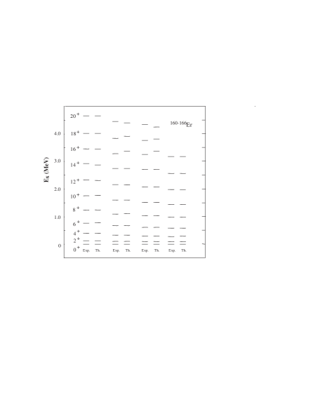
Figure 18: Experimental and theoretical energy levels in some even–even Er isotopes calculated with a single broken pair using the code SU3su2 [55, 56]. The spectrum of ¹⁶⁰Er is to the left and that of ¹⁶⁶Er to the right.

In Fig. 18, we present the results of a $u=2$ calculation of the energy levels up to $J=20$ for the even–even isotopes ^160-166Er [56]. The inclusion of a single broken pair in the $SU_{3}$ symmetry limit leads to a quantitative description of the spectrum. We do not show results for $B(E2)$ values from these calculations because that work is still in progress. Preliminary indicatons are that the inclusion of a single broken pair leads to a substantial increase in the $B(E2)$ strengths at higher spins, but the calculated values are still low in the angular momentum 10–20 region, suggesting that configurations having two broken pairs may be important for a quantitative description of $B(E2)$ values near angular momentum 20 for rare earth nuclei.

7 Conclusions

The Fermion Dynamical Symmetry Model (FDSM) provides a systematic method for truncating the spherical shell model. In this scheme, a valence space is selected using energy considerations and principles of dynamical symmetry are then used to radically truncate the valence space. We term this a symmetry-dictated truncation. The resulting truncated space permits systematic shell model calculations to be implemented for all heavy nuclei. Since the space has been severely truncated, the corresponding interactions are highly effective with respect to the original shell model. Thus, the first step in systematic calculations with this truncation scheme is to determine the appropriate FDSM effective interaction for each valence space. Although it is of considerable interest in the longer term to relate such effective interactions to standard shell model ones, the most practical initial way to determine the required interaction is to construct it phenomenologically by viewing its matrix elements as parameters to be constrained by a carefully chosen data set. We have presented examples of systematic FDSM calculations that have been used to determine an effective interaction appropriate for configurations in heavy nuclei with no broken pairs. This interaction appears to be simple and to have a rather weak dependence on particle number within major-shell valence spaces. Calculations using this interaction reproduce low-lying spectra, moments, and transition rates for broad ranges of nuclei that exhibit varied collective behavior: axial rotors, anharmonic vibrators, and gamma-soft rotors. Finally, we have presented an initial extension of this approach to include broken pairs in the configuration space. These results constitute a practical demonstration that systematic shell model calculations are now feasible for very heavy nuclei far removed from closed shells. The primary remaining task is to systematize and refine the interaction over all mass numbers through a detailed series of numerical calculations.

Acknowledgements.

Nuclear physics research at Drexel University is supported by the National Science Foundation. Nuclear physics research at Chung Yuan Christian University is supported by the National Science Council of the ROC. Nuclear physics research at the University of Tennessee is supported by the U. S. Department of Energy through Contracts No. DE–FG05–87ER40361 and DE–FG05–93ER40770. Oak Ridge National Laboratory is managed by Lockheed Martin Energy Systems, Inc. for the U. S. Department of Energy under Contract No. DE–AC05–84OR21400.

                          

                               

           

                      

                      

                  

           

                             

                          

                

                    

                             

                                 

   

                    

Figure 15: Spectra for positive-parity states in ^190-194,198Pt. Experimental levels are taken from [58, 59, 60, 61].

           

Figure 16: Experimental and calculated energy levels for the first $2^{+}$ (lower points) and $1^{+}$ (upper points) states in selected even–even rare earth nuclei where orbital $M1$ strengths have been measured. The symbols denote isotopes with the same meanings as in Fig. 17.

Figure 17: Comparison of experimental and theoretical $B(E2)$ and summed $B(M1)$ values for rare-earth nuclei as a function of $P$. The experimental results in the left column are taken from the compilation given in [46] and [62]. For comparison, curves from the same empirical relation employed there, $B(E2,M1)=a_{1}+a_{2}/[1+exp((c-P)/d)]$ are also plotted. The symbols in (c)–(c^′′) have the same meaning as in the $E2$ and $M1$ cases. The theoretical results in the second column of figures correspond to best adjustment of effective interaction parameters to reproduce spectra. The theoretical results in the third column of figures correspond to constant values of the effective interaction parameters for all nuclei examined.

                

Table 1: Experimental and Theoretical Mass Excesses in MeV for the Heaviest Elements.

${}^{256}104$	${}^{258}105$	${}^{260}106$	${}^{262}107$	${}^{264}108$	${}^{266}109$	${}^{269}110$	${}^{272}111$	Reference
94.25(03)	101.84(34)	106.60(04)	114.68(38)	119.82(30)	128.39(35)	134.80(32)	141.70(37)	Exp [63, 35]
94.15	101.98	106.8	114.82	120.02	128.16	133.31	140.49	FDSM [36]
95.90	103.41	106.87	116.10	121.28	129.44		144.83	Myers [64]
94.84	102.22	105.81	115.00	120.40	128.43		144.04	Groote [64]
95.6	102.6	106.8	114.9	120.4	127.8		142.6	Seeger [64]
94.37	101.64	105.68	114.78	120.27	128.44		143.82	Liran [64]
95.77	103.01	108.13	115.50					Möller [65]
95.69	103.11	108.12	115.71	121.09	129.04	135.51	143.44	Möller [66]
93.78	101.00	105.81	113.18	118.34	126.06	132.39	140.18	Möller [67]
93.38	100.97	105.73	113.45	118.73	126.65	133.08	140.93	Möller [68]
94.52		107.04		120.47				Patyk [69]
94.38		106.93		120.47		135.46		Cwiok [70]

Table 2: Parameters for even Xe isotopes.

Nuclei	$g_{6}$(keV)	$g^{\prime}_{5}$(keV)	$g^{\prime}_{I}$(keV)
120Xe	-60	53	11.9
122Xe	-64	59	11.9
124Xe	-68.8	64	11.9
126Xe	-73.3	71	11.9
128Xe	-78.2	79	11.9
130Xe	-100.9	100	11.9
132Xe	-106.5	122	11.9

Table 3: Parameters for odd Xe isotopes.

Nuclei	$g_{6}$(keV)	$g^{\prime}_{5}$(keV)	$g_{5}$(keV)	$g_{J}$(keV)
127Xe	-73.3	71.0	-38.0	25.0
129Xe	-78.2	79.0	-18.0	35.3
131Xe	-100.9	100.0	30.0	35.3
133Xe	-106.5	122.0	50.5	35.3
135Xe		142.1	70.6	35.3

Table 4: Parameters for odd Ba isotopes.

Nuclei	$g^{i}_{5}$(keV)	$g_{5}$(keV)	$g_{J}$(keV)
131Ba	72.5	-20	35.3
133Ba	105	-15	35.3
135Ba	90	50	35.3
137Ba	72	70	35.3

Table 5: Relative $B(E2)$ values for the even Xe isotopes.

	120Xe		124Xe		126Xe		128Xe		130Xe
$J_{i}\rightarrow J_{f}$	Exp.	Theo.	Exp.	Theo.	Exp.	Theo.	Exp.	Theo.	Exp.	Theo.
$2^{+}_{2}\rightarrow 2^{+}_{1}$	100	100	100	100	100	100	100	100	100	100
$\rightarrow 0^{+}_{1}$	5.6	5.6	3.9	3.9	1.5	1.4	1.2	1.2	0.6	0.6
$3^{+}_{1}\rightarrow 2^{+}_{2}$	100	100	100	100	100	100	100	100	100	100
$\rightarrow 4^{+}_{1}$	50	40	46	40	34	40	37	40	25	40
$\rightarrow 2^{+}_{1}$	2.7	7.1	1.6	4.9	2.0	1.85	1.0	1.5	1.4	0.72
$4^{+}_{2}\rightarrow 2^{+}_{2}$	100	100	100	100	100	100	100	100	100	100
$\rightarrow 4^{+}_{1}$	62	91	91	91	76	91	133	91	107	91
$\rightarrow 2^{+}_{1}$	—	7.11	0.4	4.91	1.0	1.83	1.7	1.49	3.2	0.97
$0^{+}_{2}\rightarrow 2^{+}_{2}$	100	100	100	100	100	100	100	100	100	100
$\rightarrow 2^{+}_{1}$	—	7.11	1	4.91	7.7	1.83	14	1.49	26	0.97

Table 6: Transition probablities in ¹²⁹Xe ($N_{1}=5$) and ¹³¹Xe ($N_{1}$=4), $\Omega_{1}=20$.

129Xe				131Xe
	$B(E2)(e^{2}b^{2})$				$B(E2)(e^{2}b^{2})$
$J_{i}\rightarrow J_{f}$	FDSM	Exp.	Ref. [71]	$J_{i}\rightarrow J_{f}$	FDSM	Exp.	Ref. [71]
$\frac{3}{2}^{+}_{{}_{1}}\rightarrow\frac{1}{2}^{+}_{{}_{1}}$	0.036		0.007	$\frac{1}{2}^{+}_{{}_{1}}\rightarrow\frac{3}{2}^{+}_{{}_{1}}$	0.0953	0.0039	0.0012
$\frac{3}{2}^{+}_{{}_{2}}\rightarrow\frac{3}{2}^{+}_{{}_{1}}$	0.0186	$<$0.0005	0.013	$\frac{5}{2}^{+}_{{}_{1}}\rightarrow\frac{1}{2}^{+}_{{}_{1}}$	0.075	0.030	0.016
$\frac{3}{2}^{+}_{{}_{2}}\rightarrow\frac{1}{2}^{+}_{{}_{1}}$	0.084	0.12	0.12	$\frac{5}{2}^{+}_{{}_{1}}\rightarrow\frac{3}{2}^{+}_{{}_{1}}$	0.004	0.10	0.10
$\frac{5}{2}^{+}_{{}_{1}}\rightarrow\frac{3}{2}^{+}_{{}_{1}}$	0.011	0.22	0.10	$\frac{3}{2}^{+}_{{}_{2}}\rightarrow\frac{3}{2}^{+}_{{}_{1}}$	0.053	0.057	0.058
$\frac{5}{2}^{+}_{{}_{1}}\rightarrow\frac{1}{2}^{+}_{{}_{1}}$	0.070	0.077	0.039	$\frac{1}{2}^{+}_{{}_{2}}\rightarrow\frac{1}{2}^{+}_{{}_{1}}$	0.0000
$\frac{1}{2}^{+}_{{}_{2}}\rightarrow\frac{3}{2}^{+}_{{}_{2}}$	0.028			$\frac{1}{2}^{+}_{{}_{2}}\rightarrow\frac{3}{2}^{+}_{{}_{1}}$	0.124	0.048	0.115
$\frac{1}{2}^{+}_{{}_{2}}\rightarrow\frac{3}{2}^{+}_{{}_{1}}$	0.14	0.044	0.12	$\frac{7}{2}^{+}_{{}_{1}}\rightarrow\frac{5}{2}^{+}_{{}_{1}}$	0.028	0.005	0.0013
$\frac{1}{2}^{+}_{{}_{2}}\rightarrow\frac{1}{2}^{+}_{{}_{1}}$	0.0000			$\frac{7}{2}^{+}_{{}_{1}}\rightarrow\frac{3}{2}^{+}_{{}_{1}}$	0.043	0.081	0.082
$\frac{5}{2}^{+}_{{}_{2}}\rightarrow\frac{1}{2}^{+}_{{}_{1}}$	0.004	0.057	0.071	$\frac{3}{2}^{+}_{{}_{3}}\rightarrow\frac{3}{2}^{+}_{{}_{1}}$	0.025	0.027	0.017
$\frac{3}{2}^{+}_{{}_{3}}\rightarrow\frac{1}{2}^{+}_{{}_{1}}$	0.056	0.0032	0.0056	$\frac{5}{2}^{+}_{{}_{2}}\rightarrow\frac{3}{2}^{+}_{{}_{2}}$	0.004	$<$0.031	0.0011
$\frac{3}{2}^{+}_{{}_{4}}\rightarrow\frac{1}{2}^{+}_{{}_{1}}$	0.0133	0.0030	0.0004	$\frac{5}{2}^{+}_{{}_{2}}\rightarrow\frac{1}{2}^{+}_{{}_{1}}$	0.071	0.068	0.056
				$\frac{5}{2}^{+}_{{}_{2}}\rightarrow\frac{3}{2}^{+}_{{}_{1}}$	0.014	0.013	0.043
				$\frac{7}{2}^{+}_{{}_{2}}\rightarrow\frac{3}{2}^{+}_{{}_{1}}$	0.124	0.005	0.026

Table 7: Parameters for the Pt calculations.

Mass=	190	192	194	196	198
$N_{1\nu}$	6	6	5	4	3
$B_{2\pi\nu}$	$-386$	$-386$	$-386$	$-386$	$-386$
$B_{2\pi}$	48	48	48	48	48
$G_{0\nu}$	$-49$	$-49$	$-49$	$-49$	$-49$
$G_{0\pi}$	$-10$	$-3$	$-5$	$-18$	$-50$
$B_{2\nu}$	36	53	74	97	100
$e_{\pi}$	0.17	0.17	0.15	0.16	0.18
$e_{\nu}$	0.19	0.19	0.15	0.14	0.19
$g_{\pi}=0.62,~{}~{}~{}~{}~{}~{}~{}~{}~{}~{}~{}~{}~{}~{}~{}~{}g_{\nu}=0$
$\beta_{0\pi}=13\times 10^{-3}\mbox{fm},~{}~{}~{}~{}\beta_{0\nu}=-1.2\times 10^{-3}\mbox{fm}$

Table 8: Comparison of $B(E2)$ values for ¹⁹⁶Pt.

$J_{i}\rightarrow J_{f}$	$B(E2)_{\scriptsize\rm exp}^{(a)}$	$B(E2)^{(d)}_{\scriptsize\rm exp}$	$SO(6)$ limit(f)	IBM–2(e)	IBM–1(g)	FDSM
$2_{1}^{+}\rightarrow 0_{1}^{+}$	0.288(14)	0.274(1)	0.288	0.289	0.288	0.195
$4_{1}^{+}\rightarrow 2_{1}^{+}$	0.403(32)	0.410(6)	0.378	0.395	0.393	0.248
$6_{1}^{+}\rightarrow 4_{1}^{+}$	0.421(116)	0.450(28)	0.384	0.409	0.423	0.215
$8_{1}^{+}\rightarrow 6_{1}^{+}$	0.577(58)	—	0.341	0.325	0.416	0.139
$2_{2}^{+}\rightarrow 2_{1}^{+}$	0.350(31)	0.370(5)	0.378	0.40	0.303	0.262
$2_{2}^{+}\rightarrow 0_{1}^{+}$	$<2.0\times 10^{-6}$ (b)	—	0	0.001	0.004	0.0001
$0_{2}^{+}\rightarrow 2_{2}^{+}$	0.142(77)	0.1(1)	0.385	0.466	0.375	0.268
$0_{2}^{+}\rightarrow 2_{1}^{+}$	0.033(7) (b)	0.028(5)	0	0.026	0.007	0.021
$4_{2}^{+}\rightarrow 4_{1}^{+}$	0.193(97) (b)	0.084(14)	0.183	0.206	0.171	0.121
$4_{2}^{+}\rightarrow 2_{2}^{+}$	0.177(35) (b)	0.18(2)	0.201	0.206	0.199	0.112
$4_{2}^{+}\rightarrow 2_{1}^{+}$	0.0030(10) (b)	0.001(2)	0	0.006	0.004	0.001
$6_{2}^{+}\rightarrow 6_{1}^{+}$	0.085(121) (b)	—	0.108	0.12	0.11	0.075
$6_{2}^{+}\rightarrow 4_{2}^{+}$	0.350(102) (b)	–	0.232	0.201	0.25	0.056
$6_{2}^{+}\rightarrow 4_{1}^{+}$	0.0037(16) (b)	-	0	0.017	0.001	0.031
$2_{{}_{3}}^{+}\rightarrow 2_{1}^{+}$	0.0009(15) (b)	–	0	0.004	$7.2\times 10^{-6}$	0.004
$0_{{}_{3}}^{+}\rightarrow 2_{1}^{+}$	$<0.034$ (c)	—	0	0.067	0.003	0.010
(a) $B(E2)_{\scriptsize\rm exp}$ are taken from H. H. Bolotin et al., Nucl. Phys. A370 (1981)146   .
(b) Data are from A. Mauthofer et al., Z. Phys. A336 (1990) 263.
(c) Data are from H. G. Börner et al., Phys. Rev. C42 (1990)R2271.
(d) $B(E2)_{\scriptsize\rm exp}$ are taken from C. S. Lim et al., Nucl.  Phys., A548 (1992) 308.
(e) Calc. from Bijker et al., Nucl. Phys. A344 (1980) 207.
(f) For $O(6)$ limit, $e=0.155(eb)$.

Table 9: Comparison of experimental and theoretical g-factors in ^190-198Pt.

		$2^{+}_{1}$			$4^{+}_{1}$			$2^{+}_{2}$
isotope	exp.(a)	IBM(c)	FDSM	exp.(a)	IBM	FDSM	exp.(a)	IBM	FDSM
190			0.137			0.092			0.121
192	0.318(17)	0.23	0.182	0.281(30)		0.126	0.278(46)		0.139
194	0.295(10)	0.27	0.239	0.279(31)		0.171	0.281(55)		0.178
196	0.295(10)	0.32	0.268	0.345(40)		0.213	0.271(45)(b)		0.207
198	0.293(34)(b)	0.40	0.26	0.307(54)(b)		0.170	0.307(54)(b)		0.213
(a) Data are taken from F. Brandolini et al., Nucl. Phys. A536 (1992) 366.
(b) Data are taken from A. E. Stuchbery, G. J. Lampard and H. H. Bolotin,
(b) Nucl. Phys. A365 (1981) 317; A528 (1991) 447.
(c) IBA–2 calc. from M. Sambataro, et al., Nucl. Phys. A423 (1984) 333.

Table 10: Experimental and theoretical changes of charge radii for ^190-198Pt isotopes.

	$\delta<r^{2}>(10^{-3}\mbox{ fm})$										$\Delta<r^{2}>(10^{-3}\mbox{ fm})$
	190		192		194		196		198		192-190	194-192	196-194	198-196
	$2^{+}_{1}$	$2^{+}_{2}$	$2^{+}_{1}$	$2^{+}_{2}$	$2^{+}_{1}$	$2^{+}_{2}$	$2^{+}_{1}$	$2^{+}_{2}$	$2^{+}_{1}$	$2^{+}_{2}$
FDSM	4.48	3.22	3.84	4.76	3.16	4.93	2.66	5.54	2.14	3.68	74	75	71	69
IBM					3.62	5.08	2.55
Exp.(a)					3.45	3.57	4.49				65	67	74	80
(a) Isomer shifts are taken from R. Engfer et al., Nucl. Data Tables, 14 (1974) 509;
(a) Isotope shifts are taken from Th. Hilberath et al., Z. Phys., A342 (1992) 1.

References

- [1] M. Vallieres, Nucl. Phys. A570, (1993).
- [2] B. Brown, A. Etchegoyen, and W. Rae, The computer code OXBASH, MSU–NSCL number 524.
- [3] X.-W. Pan et al., In Press, Phys. Rep. (1995).
- [4] C. W. Johnson et al., Phys. Rev. Lett. 69, 3147 (1992).
- [5] E. Ormand et al., Phys. Rev. C49, 1422 (1994).
- [6] K. W. Schmid, R. Grummer, M. Kyotoku, and A. Faessler, Nucl. Phys. A452, 493 (1986).
- [7] K. Hara and Y. Sun, Nucl. Phys. A529, 445 (1991).
- [8] C.-L. Wu, D. H. Feng, and M. W. Guidry, Advances in Nuclear Physics 21, 227 (1994).
- [9] M. W. Guidry, in Nuclear Physics in the Universe, edited by M. W. Guidry and M. R. Strayer (IOP Publishing, Bristol, 1993), p. 453.
- [10] M. W. Guidry, Nucl. Phys. A570, 109c (1993).
- [11] F. Iachello and A. Arima, The Interacting Boson Model (Cambridge University Press, Cambridge, 1987).
- [12] K. Hara and S. Iwasaki, Nucl. Phys. A348, 200 (1980).
- [13] M. Kirson, in Proc. Conference on the Nuclear Shell Model, edited by M. Vallieres and B. H. Wildenthal (World Scientific, Singapore, 1985), p. 290.
- [14] C.-L. Wu et al., Phys. Rev. C36, 1157 (1987).
- [15] J.-Q. Chen, D. H. Feng, M. W. Guidry, and C. L. Wu, Phys. Rev. C44, 559 (1991).
- [16] I. Talmi, Helv. Phys. Acta 25, 185 (1952).
- [17] B. H. Wildenthal, in Proc. Conf. on the Nuclear Shell Model, edited by M. Vallieres and B. H. Wildenthal (World Scientific, Singapore, 1985), p. 346.
- [18] B. A. Brown and B. H. Wildenthal, Ann. Rev. Nuc. Part. Sci. 38, 29 (1988).
- [19] J. N. Ginocchio, Ann. Phys. 126, 234 (1980).
- [20] C.-L. Wu, D. H. Feng, and M. W. Guidry, Ann. Phys. 222, 187 (1993).
- [21] M. W. Guidry, in Nuclear Physics of our Times, edited by R. V. Ramayya (World Scientific, Singapore, 1993), p. 277.
- [22] C.-L. Wu et al., Phys. Rev. C51, R1086 (1995).
- [23] C.-L. Wu et al., Phys. Lett. B168, 313 (1986).
- [24] J. P. Elliott, Proc. Roy. Soc. A245, 128, 562 (1958).
- [25] K. T. Hecht and A. Adler, Nucl. Phys. A137, 129 (1969).
- [26] A. Arima, M. Harvey, and K. Shimizu, Phys. Lett. B30, 517 (1969).
- [27] H. Wu and M. Vallieres, Phys. Rev. C39, 1066 (1989).
- [28] M. Valliéres and H. Wu, in Computational Nuclear Physics 1, ed. by K. Langanke, et al (Springer–Verlag) p. 1, 1991.
- [29] Z.-P. Li, M. W. Guidry, C.-L. Wu, and D. H. Feng, Int. J. Modern Phys. E3, 1119 (1994).
- [30] M. W. Guidry and C.-L. Wu, Int. J. Mod. Phys. E (supp 1993) 2, 17 (1993).
- [31] M. W. Guidry, C. L. Wu, and D. H. Feng, Ann. Phys. 242, 135 (1995).
- [32] G. Münzenberg et al., Zeit. Phys. A300, 107 (1981).
- [33] G. Münzenberg et al., Zeit. Phys. A309, 89 (1982).
- [34] G. Münzenberg et al., Zeit. Phys. A317, 235 (1984).
- [35] S. Hoffmann et al., Zeit. Phys. A350, 277 (1995).
- [36] X.-L. Han, C.-L. Wu, M. W. Guidry, and D. H. Feng, Phys. Rev. C45, 1127 (1992).
- [37] M. W. Guidry, C.-L. Wu, and D. H. Feng, To Be Published .
- [38] R.-P. Wang, F.-K. Thielemann, D. H. Feng, and C.-L. Wu, Phys. Lett. B284, 196 (1992).
- [39] J.-Q. Chen, D. H. Feng, and C.-L. Wu, Phys. Rev. C34, 2269 (1986).
- [40] X.-W. Pan et al., Phys. Rev. C, Submitted (1995).
- [41] X.-W. Pan, D. H. Feng, J.-Q. Chen, and M. W. Guidry, Phys. Rev. C49, 2493 (1994).
- [42] D. H. Feng et al., Phys. Rev. 48, R1488 (1993).
- [43] J. L. Ping et al., Phys. Rev. C , Submitted (1995).
- [44] T. Otsuka, A. Arima, F. Iachello, and I. Talmi, Phys. Lett. B66, 20 (1977).
- [45] R. F. Casten and D. D. Warner, Rev. Mod. Phys. 60, 389 (1988).
- [46] C. Rangacharyulu et al., Phys. Rev. C43, R949 (1991).
- [47] J. N. Ginocchio, Phys. Lett. B265, 6 (1991).
- [48] R. F. Casten, D. S. Brenner, and P. E. Haustein, Phys. Rev. Lett. 58, 658 (1987).
- [49] M. W. Guidry et al., Phys. Lett. B176, 1 (1986).
- [50] M. W. Guidry et al., Phys. Lett. B187, 210 (1987).
- [51] C.-L. Wu, Nucl. Phys. A520, 459c (1990).
- [52] H. Wu et al., Phys. Lett. B193, 163 (1987).
- [53] H. Wu, D. H. Feng, C.-L. Wu, and M. W. Guidry, Phys. Lett. B198, 119 (1987).
- [54] H. Wu, C.-L. Wu, D. H. Feng, and M. W. Guidry, Phys. Rev. C37, 1739 (1988).
- [55] Y.-M. Di, N. Yoshida, and X. W. Pan, Code SU3u2 (unpublished).
- [56] X. W. Pan et al., The Broken Pair Effect on the Moment of Inertia in the Fermion Dynamical Symmetry Model (unpublished).
- [57] J. A. Cizewski et al., Phys. Rev. Lett. 40, 167 (1978).
- [58] B. Singh, Nucl. Data Sheets 56, 75 (1989).
- [59] B. Singh, Nucl. Data Sheets 61, 243 (1990).
- [60] C. M. Zhou, Nucl. Data Sheets 60, 527 (1990).
- [61] V. S. Shirley, Nucl. Data Sheets 64, 205 (1991).
- [62] S. Raman, C. W. N. Jr., S. Kahane, and K. H. Bhatt, At. Data Nucl. Data Tables 42, 1 (1987).
- [63] G. Audi and A. H. Wapstra, Nucl. Phys. A565, 1 (1993).
- [64] Atomic and Nucl. Data Tables 17, 411 (1976).
- [65] P. Möller and J. R. Nix, Atomic and Nuc. Data Tables 26, 105 (1981).
- [66] P. Möller and J. R. Nix, Atomic and Nuc. Data Tables 39, 213 (1988).
- [67] P. Möller and J. R. Nix, Atomic and Nuc. Data Tables 39, 225 (1988).
- [68] P. Möller, J. R. Nix, W. D. Myers, and W. J. Swiatecki, Atomic and Nuc. Data Tables 59, 185 (1995).
- [69] Z. Patyk and A. Sobiczewski, Nucl. Phys. A533, 132 (1991).
- [70] S. Cwiok, S. Hofmann, and W. Nazarewicz, Nucl. Phys. A573, 356 (1994).
- [71] J. Jolie, K. Heyde, P. V. Isacker, and A. Frank, Nucl. Phys. A466, 1 (1987).
- [1] M. Vallieres, Nucl. Phys. A570, (1993); M. Vallières and A. Novoselsky, Drexel University Shell Model (DUSM) code), (1994).
- [2] B. Brown, A. Etchegoyen, and W. Rae, The computer code OXBASH, MSU–NSCL number 524.
- [3] X.-W. Pan et al., In Press, Phys. Rep. (1995).
- [4] C. W. Johnson et al., Phys. Rev. Lett. 69, 3147 (1992).
- [5] E. Ormand et al., Phys. Rev. C49, 1422 (1994).
- [6] K. W. Schmid, R. Grummer, M. Kyotoku, and A. Faessler, Nucl. Phys. A452, 493 (1986).
- [7] K. Hara and Y. Sun, Nucl. Phys. A529, 445 (1991).
- [8] C.-L. Wu, D. H. Feng, and M. W. Guidry, Advances in Nuclear Physics 21, 227 (1994).
- [9] M. W. Guidry, in Nuclear Physics in the Universe, edited by M. W. Guidry and M. R. Strayer (IOP Publishing, Bristol, 1993), p. 453.
- [10] M. W. Guidry, Nucl. Phys. A570, 109c (1993).
- [11] F. Iachello and A. Arima, The Interacting Boson Model (Cambridge University Press, Cambridge, 1987).
- [12] K. Hara and S. Iwasaki, Nucl. Phys. A348, 200 (1980).
- [13] M. Kirson, in Proc. Conference on the Nuclear Shell Model, edited by M. Vallieres and B. H. Wildenthal (World Scientific, Singapore, 1985), p. 290.
- [14] C.-L. Wu et al., Phys. Rev. C36, 1157 (1987).
- [15] J.-Q. Chen, D. H. Feng, M. W. Guidry, and C. L. Wu, Phys. Rev. C44, 559 (1991).
- [16] I. Talmi, Helv. Phys. Acta 25, 185 (1952).
- [17] B. H. Wildenthal, in Proc. Conf. on the Nuclear Shell Model, edited by M. Vallieres and B. H. Wildenthal (World Scientific, Singapore, 1985), p. 346.
- [18] B. A. Brown and B. H. Wildenthal, Ann. Rev. Nuc. Part. Sci. 38, 29 (1988).
- [19] J. N. Ginocchio, Ann. Phys. 126, 234 (1980).
- [20] C.-L. Wu, D. H. Feng, and M. W. Guidry, Ann. Phys. 222, 187 (1993).
- [21] M. W. Guidry, in Nuclear Physics of our Times, edited by R. V. Ramayya (World Scientific, Singapore, 1993), p. 277.
- [22] C.-L. Wu et al., Phys. Rev. C51, R1086 (1995).
- [23] C.-L. Wu et al., Phys. Lett. B168, 313 (1986).
- [24] J. P. Elliott, Proc. Roy. Soc. A245, 128, 562 (1958).
- [25] K. T. Hecht and A. Adler, Nucl. Phys. A137, 129 (1969).
- [26] A. Arima, M. Harvey, and K. Shimizu, Phys. Lett. B30, 517 (1969).
- [27] H. Wu and M. Vallieres, Phys. Rev. C39, 1066 (1989).
- [28] M. Valliéres and H. Wu, in Computational Nuclear Physics 1, ed. by K. Langanke, et al (Springer–Verlag) p. 1, 1991.
- [29] Z.-P. Li, M. W. Guidry, C.-L. Wu, and D. H. Feng, Int. J. Modern Phys. E3, 1119 (1994).
- [30] M. W. Guidry and C.-L. Wu, Int. J. Mod. Phys. E (supp 1993) 2, 17 (1993).
- [31] M. W. Guidry, C. L. Wu, and D. H. Feng, Ann. Phys. 242, 135 (1995).
- [32] G. Münzenberg et al., Zeit. Phys. A300, 107 (1981).
- [33] G. Münzenberg et al., Zeit. Phys. A309, 89 (1982).
- [34] G. Münzenberg et al., Zeit. Phys. A317, 235 (1984).
- [35] S. Hoffmann et al., Zeit. Phys. A350, 277 (1995).
- [36] X.-L. Han, C.-L. Wu, M. W. Guidry, and D. H. Feng, Phys. Rev. C45, 1127 (1992).
- [37] M. W. Guidry, C.-L. Wu, and D. H. Feng, To Be Published .
- [38] R.-P. Wang, F.-K. Thielemann, D. H. Feng, and C.-L. Wu, Phys. Lett. B284, 196 (1992).
- [39] J.-Q. Chen, D. H. Feng, and C.-L. Wu, Phys. Rev. C34, 2269 (1986).
- [40] X.-W. Pan et al., Phys. Rev. C, Submitted (1995).
- [41] X.-W. Pan, D. H. Feng, J.-Q. Chen, and M. W. Guidry, Phys. Rev. C49, 2493 (1994).
- [42] D. H. Feng et al., Phys. Rev. 48, R1488 (1993).
- [43] J. L. Ping et al., Phys. Rev. C , Submitted (1995).
- [44] T. Otsuka, A. Arima, F. Iachello, and I. Talmi, Phys. Lett. B66, 20 (1977).
- [45] R. F. Casten and D. D. Warner, Rev. Mod. Phys. 60, 389 (1988).
- [46] C. Rangacharyulu et al., Phys. Rev. C43, R949 (1991).
- [47] J. N. Ginocchio, Phys. Lett. B265, 6 (1991).
- [48] R. F. Casten, D. S. Brenner, and P. E. Haustein, Phys. Rev. Lett. 58, 658 (1987).
- [49] M. W. Guidry et al., Phys. Lett. B176, 1 (1986).
- [50] M. W. Guidry et al., Phys. Lett. B187, 210 (1987).
- [51] C.-L. Wu, Nucl. Phys. A520, 459c (1990).
- [52] H. Wu et al., Phys. Lett. B193, 163 (1987).
- [53] H. Wu, D. H. Feng, C.-L. Wu, and M. W. Guidry, Phys. Lett. B198, 119 (1987).
- [54] H. Wu, C.-L. Wu, D. H. Feng, and M. W. Guidry, Phys. Rev. C37, 1739 (1988).
- [55] Y.-M. Di, N. Yoshida, and X. W. Pan, Code SU3u2 (unpublished).
- [56] X. W. Pan et al., The Broken Pair Effect on the Moment of Inertia in the Fermion Dynamical Symmetry Model (unpublished).
- [57] J. A. Cizewski et al., Phys. Rev. Lett. 40, 167 (1978).
- [58] B. Singh, Nucl. Data Sheets 56, 75 (1989).
- [59] B. Singh, Nucl. Data Sheets 61, 243 (1990).
- [60] C. M. Zhou, Nucl. Data Sheets 60, 527 (1990).
- [61] V. S. Shirley, Nucl. Data Sheets 64, 205 (1991).
- [62] S. Raman, C. W. N. Jr., S. Kahane, and K. H. Bhatt, At. Data Nucl. Data Tables 42, 1 (1987).
- [63] G. Audi and A. H. Wapstra, Nucl. Phys. A565, 1 (1993).
- [64] Atomic and Nucl. Data Tables 17, 411 (1976).
- [65] P. Möller and J. R. Nix, Atomic and Nuc. Data Tables 26, 105 (1981).
- [66] P. Möller and J. R. Nix, Atomic and Nuc. Data Tables 39, 213 (1988).
- [67] P. Möller and J. R. Nix, Atomic and Nuc. Data Tables 39, 225 (1988).
- [68] P. Möller, J. R. Nix, W. D. Myers, and W. J. Swiatecki, Atomic and Nuc. Data Tables 59, 185 (1995).
- [69] Z. Patyk and A. Sobiczewski, Nucl. Phys. A533, 132 (1991).
- [70] S. Cwiok, S. Hofmann, and W. Nazarewicz, Nucl. Phys. A573, 356 (1994).
- [71] J. Jolie, K. Heyde, P. V. Isacker, and A. Frank, Nucl. Phys. A466, 1 (1987).