Multifragmentation calculated with
relativistic forces

1. Introduction

In molecular dynamics simulations of heavy-ion collisions at intermediate energies (300 MeV/u – 2 GeV/u) it is still an open question question, which kind of forces should be used for the long range part of the nucleon-nucleon interaction which builds up the mean field. The Skyrme forces, which work very well for lower energies are not relativistically invariant. There are attempts to extend non-relativistic two-body potentials to higher velocities by requiring approximate Lorentz invariance [1, 2, 3, 4]. Our aim is to derive from a relativistic lagrangian of the Walecka type a covariant Lagrange function for point-like particles which is suited for molecular dynamics and still has the saturation property of the original lagrangian. It should then be applicable in transport theories as for example QMD or BUU and should give reasonable results even at lower energies (50 – 200 MeV/u).

In Section 2 the relativistic Hamilton function is derived in the small acceleration approximation [5] from a many-body Lagrange function and it is expressed in terms of positions and canonical momenta of the particles. In Section 3 the QMD procedure is described, while in Section 4 we present our QMD calculations for fragment distributions in O + Br collisions at different energies and compare the calculated results with the experimental data. A few years ago the analogue calculation was done [6] with the Skyrme interaction, which is explicitly density dependent. It is interesting to compare those results with the new forces presented in this paper in order to see how far they can describe saturation and low energy phenomena.

The intention is, however, to go to intermediate energies, where QMD is more appropriate because quantum aspects like the Pauli principle or the uncertainty relation are expected to be less important.

2. Relativistic equations of motion for nucleons

In this section we are deriving the relativistic equations of motion for the mean 4-positions and the mean 4-momenta of the nucleons. We start from a field theoretical lagrangian of the following type

$${\cal L}(x) = \bar{\psi}(x)\Big{(}\gamma^{\alpha}i\partial_{\alpha}-m^{*}\left(\phi(x)\right)\Big{)}\psi(x)$$ (1)

$$- g_{\rm v}\bar{\psi}(x)\gamma^{\alpha}\psi(x)A_{\alpha}(x)$$

$$- \frac{1}{2}\phi(x)(\partial_{\alpha}\partial^{\alpha}+\mu^{2}_{\rm s})\phi(x)$$

$$+ \frac{1}{2}A^{\alpha}(x)(\partial_{\beta}\partial^{\beta}+\mu^{2}_{\rm v})A_{\alpha}(x)\ ,$$

where we allow for two different ways to couple the scalar field [7]. If $m^{*}(\phi)=m-g_{\rm s}\phi$ we obtain the Walecka lagrangian, whereas for $m^{*}(\phi)=\left(m+g_{\rm s}\phi\right)^{-1}$ we deal with the lagrangian proposed by Zimányi and Moszkowski [8]. (In the following, if not expressed explicitly otherwise, we use units such that $\ \hbar=c=1$.)

The field equations are

$$\Big{\{}(i\partial_{\alpha}-g_{\rm v}A_{\alpha}(x))-m^{*}\left(\phi(x)\right)\Big{\}}\ \psi(x)=0$$ (2)

for the nucleons,

$$(\partial^{\beta}\partial_{\beta}+\mu^{2}_{\rm s})\ \phi(x)=-\ {d\over{d\phi}}m^{*}\left(\phi(x)\right)\ \bar{\psi}(x)\psi(x)$$ (3)

for the scalar field and

$$(\partial^{\beta}\partial_{\beta}+\mu_{\rm v}^{2})\ A^{\alpha}(x)=g_{\rm v}\,\bar{\psi}(x)\gamma^{\alpha}\psi(x)$$ (4)

for the vector field.

In the mean-field approximation the source terms are replaced by their expectation values $\bar{\psi}(x)\psi(x)\Rightarrow\rho_{\rm s}(x)$ and $\bar{\psi}(x)\gamma^{\alpha}\psi(x)\Rightarrow j^{\alpha}(x)$ so that the scalar and vector fields become classical fields. For classical fields, however, an arbitrarily weak time dependence in the scalar density $\rho_{\rm s}(x)$ or current density $j^{\alpha}(x)$ results in a radiation field which travels away from the nucleons. The total field energy in the radiation may even be less than the masses of the field quanta. Since the fields are only effective fields, and for the scalar field there is no corresponding elementary particle, the physical meaning of this radiation is obscure.

As we are using the relativistic scalar and vector fields only for the mean-field part of the nuclear interaction we follow the suggestion [1, 9] to exclude radiation of fictitious mesons from the very beginning by using the action-at-a-distance formulation with the symmetric Green’s function of Wheeler and Feynman [10].

$$G_{\rm s,v}(x-y)=\frac{1}{2}\Big{(}G^{advanced}_{\rm s,v}(x-y)+G^{retarded}_{\rm s,v}(x-y)\Big{)}\$$ (5)

The formal solution of the wave Eq. (3) (for $m^{*}=m-g_{\rm s}\phi$)

$$\phi(x)=g_{\rm s}\int\!d^{4}y\ G_{\rm s}(x-y)\bar{\psi}(y)\psi(y)$$ (6)

and of Eq. (4)

$$A^{\alpha}(x)=g_{\rm v}\int\!d^{4}y\ G_{\rm v}(x-y)\bar{\psi}(y)\gamma^{\alpha}\psi(y)$$ (7)

fulfills the desired boundary condition of vanishing incoming and outgoing free fields.

Eliminating the fields from the lagrangian (1) leads to the non-local action which contains only nucleon variables:

$$\int d^{4}x\ {\cal L}(x) = \int d^{4}x\ \bar{\psi}(x)(\gamma^{\alpha}i\partial_{\alpha}-M)\psi(x)$$ (8)

$$+ \frac{1}{2}g_{\rm s}^{2}\int d^{4}x\ d^{4}y\ \bar{\psi}(x)\psi(x)\,G_{\rm s}(x-y)\,\bar{\psi}(y)\psi(y)$$

$$- \frac{1}{2}g_{\rm v}^{2}\int d^{4}x\ d^{4}y\ \bar{\psi}(x)\gamma^{\alpha}\psi(x)\,G_{\rm v}(x-y)\,\bar{\psi}(y)\gamma_{\alpha}\psi(y)$$

If quantum effects are negligible the scalar density and vector current density can be represented in terms of the world lines of the nucleons as

$$\rho_{\rm s}(x):=\bar{\psi}(x)\psi(x) \rightarrow \sum_{\rm j=1}^{\rm A}\int\!d\tau^{\ }_{\rm j}\ \delta^{4}(x-r_{\rm j}(\tau^{\ }_{\rm j}))$$ (9)

$$j^{\mu}(x):=\bar{\psi}(x)\gamma^{\mu}\psi(x) \rightarrow \sum_{\rm j=1}^{\rm A}\int\!d\tau^{\ }_{\rm j}\ \delta^{4}(x-r_{\rm j}(\tau^{\ }_{\rm j}))\,u^{\mu}_{\rm j}(\tau^{\ }_{\rm j})\ ,$$ (10)

where $r_{\rm j}(\tau^{\ }_{\rm j})$ denotes the world line of the nucleon $j$ at its proper time $\tau^{\ }_{\rm j}$ and $u_{\rm j}(\tau^{\ }_{\rm j})$ its 4-velocity. Nucleons in nuclei can however not be localized well enough for treating them as classical particles on world lines. The Fermi momentum sets a limit to the radius of the nucleon wave packet in coordinate space which is of the order of 2 fm. These effects, the Pauli principle and other quantum effects, are properly taken care of in Antisymmetrized Molecular Dynamics (AMD) [11] and in Fermionic Molecular Dynamics (FMD) [12]. However, presently neither the AMD nor the FMD equations of motion can be solved numerically for large systems like gold on gold. Therefore, we mimic the finite size effect of the wave packets by folding the finally obtained forces with gaussian density distributions for the nucleons. This ”smearing” provides also the prescription how to eliminate strong forces at short distances which are taken care of by the random forces of the collision term.

Therefore, the forces to be derived in the following are only meant to represent the long range part of the nuclear interactions which constitute a mean field. In this sense $r_{\rm j}(\tau^{\ }_{\rm j})$ is the mean world line of the nucleon and $u_{\rm j}(\tau^{\ }_{\rm j})$ its mean 4-velocity.

Using the representation (9) the scalar field at a space-time point $x$, for example is given by integrals over past and future proper times $\tau^{\ }_{\rm j}$ as

$$\phi(x)=g_{\rm s}\sum_{\rm j=1}^{\rm A}\int\!d\tau^{\ }_{\rm j}\ G_{\rm s}(x-r_{\rm j}(\tau^{\ }_{\rm j}))\ .$$ (11)

By identifying the following expressions with their representation in terms of mean positions and mean momenta of the nucleons

$$\int d^{4}x\ d^{4}y\ \bar{\psi}(x)\psi(x)\,G_{\rm s}(x-y)\,\bar{\psi}(y)\psi(y) \rightarrow$$ (12)

$$\mbox{}\sum^{\rm A}_{\stackrel{{\scriptstyle{\scriptstyle\rm i,j=1}}}{{\rm i\neq j}}}\int\!d\tau_{i}d\tau^{\ }_{\rm j}\ G_{\rm s}(r_{\rm i}(\tau^{\ }_{\rm i})-r_{\rm j}(\tau^{\ }_{\rm j}))\quad,$$

$$\int d^{4}x\ d^{4}y\ \bar{\psi}(x)\gamma^{\alpha}\psi(x)\,G_{\rm v}(x-y)\,\bar{\psi}(y)\gamma_{\alpha}\psi(y) \rightarrow$$ (13)

$$\mbox{}\sum^{\rm A}_{\stackrel{{\scriptstyle{\scriptstyle\rm i,j=1}}}{{\rm i\neq j}}}\int\!d\tau^{\ }_{\rm i}d\tau^{\ }_{\rm j}\ G_{\rm v}(r_{\rm i}(\tau^{\ }_{\rm i})-r_{\rm j}(\tau^{\ }_{\rm j}))\,u_{{\rm i}\alpha}(\tau^{\ }_{\rm i})u_{\rm j}^{\alpha}(\tau^{\ }_{\rm j})$$

in the action (8) one obtains the non-instantaneous action-at-a-distance [10]

$$\int\!d^{4}x\ {\cal L}(x) \rightarrow$$

$${\cal A} = -\frac{1}{2}\sum^{\rm A}_{\rm i=1}\int\!d\tau^{\ }_{\rm i}\left(M-\lambda_{\rm i}(\tau^{\ }_{\rm i})\right)u_{\rm i}(\tau^{\ }_{\rm i})^{2}$$

$$+ \frac{1}{2}g^{2}_{\rm s}\sum^{\rm A}_{\stackrel{{\scriptstyle{\scriptstyle\rm i,j=1}}}{{\rm i\neq j}}}\int\!d\tau^{\ }_{\rm i}d\tau^{\ }_{\rm j}\ G_{\rm s}(r_{\rm i}(\tau^{\ }_{\rm i})-r_{\rm j}(\tau^{\ }_{\rm j}))$$

$$- \frac{1}{2}g^{2}_{\rm v}\sum^{\rm A}_{\stackrel{{\scriptstyle{\scriptstyle\rm i,j=1}}}{{\rm i\neq j}}}\int\!d\tau^{\ }_{\rm i}d\tau^{\ }_{\rm j}\ G_{\rm v}(r_{\rm i}(\tau^{\ }_{\rm i})-r_{\rm j}(\tau^{\ }_{\rm j}))\ u_{{\rm i}\alpha}(\tau^{\ }_{\rm i})u_{\rm j}^{\alpha}(\tau^{\ }_{\rm j})\ .$$

Lagrange multipliers $\lambda_{\rm i}(\tau^{\ }_{\rm i})$ are introduced to ensure $u_{\rm i}(\tau^{\ }_{\rm i})^{2}=1$.

The equations of motion which result from this Wheeler-Feynman action are equivalent to the classical field equations, provided the system does not radiate [10].

However, the Wheeler Feynman equations of motion cannot be solved in general as one needs to know the world lines for all the past and future times in order to calculate the fields which enter the equations for the world lines [13]. Furthermore, the no-interaction theorem states that, except in the case of non-interacting particles, there exist no covariant equations of motion for world lines in which only the 4-positions and the 4-velocities at a given time enter, as is the case in non-relativistic mechanics.

In the following this no-interaction theorem is circumvented by introducing an approximative solution to the non-local Wheeler Feynman equations of motion. This is achieved by the so called small acceleration approximation which does not assume small velocities.

2.1. Action-at-a-distance in the small acceleration approximation

In order to conserve manifest covariance of the equations of motion we introduce first the concept of a scalar time. For that the whole Minkowski space is chronologically ordered by a set of space like surfaces $S(x)$ which attribute to each 4-position $x$ a scalar time $t$ by

$$S(x)=t\ \ ,\ \ \ \mbox{with}\ \ \ \partial^{0}S(x)>0\ ,\ \partial^{0}\partial^{0}S(x)\geq 0\ .$$ (15)

The simplest choice for these isochrones, which we shall take in the following, is $S(x)=\eta_{\alpha}x^{a}$, where $\eta_{\alpha}$ is a position independent time like 4-vector.

Unlike in a collision the nucleons are not strongly accelerated by the action of the mean-field. Therefore, in order to describe the motion in the mean-field one may expand each world line around the proper time $\tau^{s}_{\rm j}$ at which the particle is at a given isochrone, i.e. $t=S(r_{\rm j}(\tau^{s}_{\rm j}))$ for each $j$.

$$r_{\rm j}^{\alpha}(\tau^{\ }_{\rm j})=r_{\rm j}^{\alpha}(\tau^{s}_{\rm j})+(\tau^{\ }_{\rm j}-\tau^{s}_{\rm j})u_{\rm j}^{\alpha}(\tau^{s}_{\rm j})+\frac{1}{2}(\tau^{\ }_{\rm j}-\tau^{s}_{\rm j})^{2}\,a_{\rm j}^{\alpha}(\tau^{s}_{\rm j})+\cdots\ .$$ (16)

This way we are defining a synchronization prescription for all particles, which does not depend on the frame. For calculating the fields we neglect of the quadratic term with the acceleration $a_{\rm j}^{\alpha}(\tau^{s}_{\rm j})$ and all higher powers which leaves us with a straight world line in the vicinity of the synchronizing time $t=S(r_{\rm j}(\tau^{s}_{\rm j}))$ (c.f. Fig. 1). This is called ”small acceleration approximation”

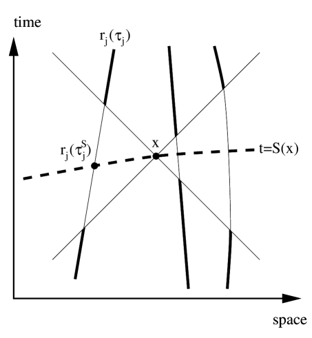
Figure 1: World lines and synchronizing hypersurface $S(x)$

The small acceleration approximation is of course best in the vicinity of $r_{\rm j}^{\alpha}(\tau^{s}_{\rm j})$ and becomes worse further away. As sketched in Fig. 1 only those parts of the world lines (thick lines), which are outside the light cone (centered at $x$), contribute to the field strength at point $x$. A world line which hits the light cone far away from $x$ may be badly approximated by Eq. (16), but for short range interactions a distant particle does not contribute anymore to the field at $x$.

Thus, the first condition for the validity of the approximation is that the range $\mu^{-1}$ is small compared to the curvature of the world lines, i.e. the inverse of the acceleration. The second condition is weak radiation, which is fulfilled when the acceleration is small compared to the meson mass $\mu$. Both conditions are actually the same, namely

$$\mid a_{\mu}a^{\mu}\mid\ \ll\ \mu^{2}.$$ (17)

The assumption of small accelerations is justified if the $\phi$ and $A^{\alpha}$ fields are only meant to be the mean-field part of the nucleon-nucleon interaction in a hadronic surrounding. The hard collisions between individual nucleons which are due to the repulsive core will cause large accelerations and also create new particles. These hard collisions cannot be described within Walecka type mean-field models. Therefore, it is consistent to regard $\phi(x)$ and $A^{\alpha}(x)$ as Hartree mean-fields which bring about only small accelerations and which are not radiated away from their sources.

Inserting the straight world line into Eq. (11) results in the easily understood situation that the field at a point $x$ is just the sum of Lorentz-boosted Yukawa potentials which are traveling along with the charges:

$$\phi(x)=\frac{g_{\rm s}}{4\pi}\sum_{\rm j}\frac{\exp\left\{-\mu_{\rm s}\sqrt{R_{\rm j}(x)^{2}}\right\}}{\sqrt{R_{\rm j}(x)^{2}}}\ ,$$ (18)

where $R_{\rm j}(x)^{2}$ is given by

$$R_{\rm j}(x)^{2}=-(x-r_{\rm j}(\tau^{s}_{\rm j}))^{2}+\left[(x^{\alpha}-r_{\rm j}^{\alpha}(\tau^{s}_{\rm j}))\,u_{{\rm j}\alpha}(\tau^{s}_{\rm j})\right]^{2}$$ (19)

The vector field is derived in an analogue fashion as

$$A^{\alpha}(x)=\frac{g_{\rm v}}{4\pi}\sum_{\rm j}\frac{\exp\left\{-\mu_{\rm v}\sqrt{R_{\rm j}(x)^{2}}\right\}}{\sqrt{R_{\rm j}(x)^{2}}}\,u_{\rm j}^{\alpha}(\tau^{s}_{\rm j})\ .$$ (20)

At this level of the approximation the causality problem with the advanced part of the Green function is not present because the retarded and the advanced fields are identically the same when they are created by charges moving on straight world lines. Therefore one may regard the fields as retarded only. In addition the unsolved problem of radiation reaction, where the radiation acts back on the world lines [14], does not occur because there are no radiation fields any more.

2.2. Instantaneous action-at-a-distance

In the spirit of the small acceleration assumption discussed in the previous section one can use the straight line expansion in the action (2. Relativistic equations of motion for nucleons) and perform the integration over $\tau^{\ }_{\rm j}$. This results in an instantaneous action-at-a-distance where the Lorentz-boosted Yukawa fields appear again and there is only one time, the scalar synchronizing time $t$.

$${\cal A}=\int\!dt\sum_{\rm i}\frac{1}{\partial_{\alpha}S(r_{\rm i}(t))u_{\rm i}^{\alpha}(t)}\Bigg{[} - \frac{1}{2}\left(M-\lambda_{\rm i}(t)\right)u_{\rm i}(t)^{2}$$

$$+ \frac{1}{2}\sum_{\stackrel{{\scriptstyle\scriptstyle\rm j}}{{\rm j\neq i}}}\frac{g^{2}_{\rm s}}{4\pi}\frac{\exp\{-\mu_{\rm s}\sqrt{R_{\rm ij}(t)^{2}}\}}{\sqrt{R_{\rm ij}(t)^{2}}}$$

$$\mbox{}-\frac{1}{2}\sum_{\stackrel{{\scriptstyle\scriptstyle\rm j}}{{\rm j\neq i}}}\frac{g^{2}_{\rm v}}{4\pi}\frac{\exp\{-\mu_{\rm v}\sqrt{R_{\rm ij}(t)^{2}}\}}{\sqrt{R_{\rm ij}(t)^{2}}}\,u_{{\rm i}\alpha}(t)u_{\rm j}^{\alpha}(t)\,\Bigg{]}$$

The four-positions $r_{\rm i}^{\alpha}(t)\equiv r_{\rm i}^{\alpha}(\tau^{\ }_{\rm i}(t))$ and 4-velocities $u_{\rm i}^{\alpha}(t)\equiv u_{\rm i}^{\alpha}(\tau^{\ }_{\rm i}(t))$ are to be taken at the same scalar synchronizing time $t$ and

$$R_{\rm ij}^{2}(t):=-(r_{\rm i}(t)-r_{\rm j}(t))^{2}+\Big{[}(r_{{\rm i}\beta}(t)-r_{{\rm j}\beta}(t))u_{\rm j}^{\beta}(t)\Big{]}^{2}$$ (22)

The small acceleration approximation together with the introduction of a synchronizing hypersurface $S(x)$ leads to an equal time lagrangian which is Lorentz-scalar and written in a manifestly covariant way.

Giving up explicit covariance and choosing $\eta=(1,0,0,0)$ in a special coordinate frame, the positions and velocities take the form

$$r_{\rm i}(\tau^{\ }_{\rm i}(t))=\Big{(}t\,,\,\vec{r}_{\rm i}(t)\Big{)}\ \ \ \mbox{and}\ \ \ u_{\rm i}(\tau^{\ }_{\rm i}(t))=\frac{1}{\sqrt{1-\vec{v}_{\rm i}^{\,2}(t)}}\Big{(}1\,,\,\vec{v}_{\rm i}(t)\Big{)}\ .$$ (23)

With that a Lagrange function ${\cal L}(\vec{r}_{\rm i}(t),\vec{v}_{\rm i}(t))$ can be defined which depends only on the independent variables and one time. Even the Lagrange multipliers $\lambda_{\rm i}(t)$ are not needed anymore if the variation is with respect to $\vec{v}_{\rm i}(t)$ instead of all four $u_{\rm i}^{\alpha}(t)$.

The advantage of the instantaneous Lagrangian is that one can define easily the hamiltonian and the total momentum, which are then strictly conserved by the equations of motion.

2.3. Hamilton equations of motion

In the following we want to express the total hamiltonian as a function of the positions $\vec{r}_{\rm i}$ and the canonical momenta $\vec{p}_{\rm i}$. Using relations (2.2. Instantaneous action-at-a-distance)-(23) the Lagrange function is

$${\cal L}= - \sum_{\rm i}\ \left[{m\over{u_{\rm i}^{0}}}+{1\over 2}\sum_{\stackrel{{\scriptstyle\scriptstyle\rm j}}{{\rm j\neq i}}}\ {g^{2}_{\rm s}\over{4\pi u_{\rm i}^{0}}}{{\rm exp}\left\{-\mu_{\rm s}\sqrt{R_{\rm ij}^{2}(t)}\right\}\over{\sqrt{R_{\rm ij}^{2}(t)}}}\right.$$

$$- \left.{1\over 2}\sum_{\stackrel{{\scriptstyle\scriptstyle\rm j}}{{\rm j\neq i}}}\ {g^{2}_{\rm v}\over{4\pi u_{\rm i}^{0}}}{{\rm exp}\left\{-\mu_{\rm v}\sqrt{R_{\rm ij}^{2}(t)}\right\}\over{\sqrt{R_{\rm ij}^{2}(t)}}}u_{\rm i\alpha}(t)u_{\rm j}^{\alpha}(t)\right]\,.$$

The canonical momenta and the energy are determined from the Lagrange function above as

$$\vec{p}_{\rm i} = {\partial{\cal L}\over{\partial\vec{v}_{\rm i}}}\quad,$$ (25)

$$E = \sum_{\rm i}{\partial{\cal L}\over{\partial\vec{v}_{\rm i}}}\vec{v}_{\rm i}-\cal{L}\quad.$$

Performing these derivatives, the energy is given by

$$E = \sum_{\rm i}\ m\ u_{\rm i}^{0}-{1\over 2}\sum_{\stackrel{{\scriptstyle\scriptstyle\rm i,j}}{{\rm j\neq i}}}\ f_{\rm ij}u_{\rm i}^{0}-{1\over 2}\sum_{\stackrel{{\scriptstyle\scriptstyle\rm i,j}}{{\rm j\neq i}}}\ \widehat{f}_{\rm ji}\ (\vec{r}_{\rm ij}\vec{u}_{\rm i})^{2}{\left(u_{\rm i}^{0}\right)^{2}\over{u_{\rm j}^{0}}}$$

$$+ {1\over 2}\sum_{\stackrel{{\scriptstyle\scriptstyle\rm i,j}}{{\rm j\neq i}}}\ g_{\rm ji}\ u_{\rm i}^{0}-{1\over 2}\sum_{\stackrel{{\scriptstyle\scriptstyle\rm i,j}}{{\rm j\neq i}}}\ g_{\rm ji}\left[u_{\rm i}^{0}\vec{u}_{\rm i}^{2}-{\left(u_{\rm i}^{0}\right)^{2}\over{u_{\rm j}^{0}}}\vec{u}_{\rm i}\vec{u}_{\rm j}\right]$$

$$+ {1\over 2}\sum_{\stackrel{{\scriptstyle\scriptstyle\rm i,j}}{{\rm j\neq i}}}\ \widehat{g}_{\rm ji}\ (\vec{r}_{\rm ij}\vec{u}_{\rm i})^{2}\left[\left(u_{\rm i}^{0}\right)^{3}-{\left(u_{\rm i}^{0}\right)^{2}\over{u_{\rm j}^{0}}}\vec{u}_{\rm i}\vec{u}_{\rm j}\right],$$

where we use the abbreviations

$$f_{\rm ij}\equiv f(R_{\rm ij})={g_{\rm s}^{2}\over{4\pi}}\ {{\rm exp}\left\{-\mu_{\rm s}\rm R_{ij}\right\}\over{R_{\rm ij}}}\quad \quad g_{\rm ij}={g_{\rm v}^{2}\over{4\pi}}\ {{\rm exp}\left\{-\mu_{\rm v}\rm R_{ij}\right\}\over{R_{\rm ij}}}\,,$$ ,

$$\widehat{f}_{\rm ji}\equiv-{1\over{R_{\rm ji}}}{d\over{dR_{\rm ji}}}f(R_{\rm ji})={g_{\rm s}^{2}\over{4\pi}}\ (1 + \mu_{\rm s}R_{\rm ji}){{\rm exp}\left\{-\mu_{\rm s}\rm R_{ji}\right\}\over{R_{\rm ji}^{3}}}\,,$$ (27)

$$R_{\rm ij}^{2}=\vec{r}_{\rm ij}^{2}+(\vec{r}_{\rm ij}\vec{u}_{\rm j})^{2}\quad \quad\vec{r}_{\rm ij}=\vec{r}_{\rm i}-\vec{r}_{\rm j}\,,$$ , (28)

and $\widehat{g}_{\rm ji}$ is defined in the same way as $\widehat{f}_{\rm ji}$. It is worthwhile to note that $f_{\rm ij}\neq f_{\rm ji}$.

The momentum of a particle looks as

$$\vec{p}_{\rm i} = m\vec{u}_{\rm i}-{1\over 2}\left(\sum_{\stackrel{{\scriptstyle\scriptstyle\rm j}}{{\rm j\neq i}}}\ f_{\rm ij}\right)\vec{u}_{\rm i}-{1\over 2}\sum_{\stackrel{{\scriptstyle\scriptstyle\rm j}}{{\rm j\neq i}}}\ \widehat{f}_{\rm ji}{u_{\rm i}^{0}\over{u_{\rm j}^{0}}}\left[\vec{r}_{\rm ij}(\vec{r}_{\rm ij}\vec{u}_{\rm i})+\vec{u}_{\rm i}(\vec{r}_{\rm ij}\vec{u}_{\rm i})^{2}\right]$$

$$+ {1\over 2}\sum_{\stackrel{{\scriptstyle\scriptstyle\rm j}}{{\rm j\neq i}}}\ \left(g_{\rm ij}+{u_{\rm i}^{0}\over{u_{\rm j}^{0}}}g_{\rm ji}\right)\vec{u}_{\rm j}-{1\over 2}\sum_{\stackrel{{\scriptstyle\scriptstyle\rm j}}{{\rm j\neq i}}}\ g_{\rm ji}\left[\left(u_{\rm i}^{0}\right)^{2}-{u_{\rm i}^{0}\over{u_{\rm j}^{0}}}\vec{u}_{\rm i}\vec{u}_{\rm j}\right]\vec{u}_{\rm i}$$

$$+ {1\over 2}\sum_{\stackrel{{\scriptstyle\scriptstyle\rm j}}{{\rm j\neq i}}}\ \widehat{g}_{\rm ji}\left[\left(u_{\rm i}^{0}\right)^{2}-{u_{\rm i}^{0}\over{u_{\rm j}^{0}}}\vec{u}_{\rm i}\vec{u}_{\rm j}\right]\left[\vec{r}_{\rm ij}(\vec{r}_{\rm ij}\vec{u}_{\rm i})+\vec{u}_{\rm i}(\vec{r}_{\rm ij}\vec{u}_{\rm i})^{2}\right]\,.$$

Let us first prove that for isotropic nuclear matter, like in the original mean-field picture [15] the vector potential will not contribute to the canonical momentum. In that case the summation can be replaced by an integration over space and momentum, folded with the phase space distribution function. Since for isotropic nuclear matter the distribution function is independent of the position, the space integral can be carried out immediately and the remaining part is written as a summation over momenta. This way we get for the Yukawa terms in nuclear matter

$$\sum_{\rm j}\ f_{\rm ij} \rightarrow \sum_{\rm j}\ \int d^{3}r_{\rm j}\ f(R_{\rm ij})=\left({g_{\rm s}\over{\mu_{\rm s}}}\right)^{2}\sum_{\rm j}\ {1\over{u_{\rm j}^{0}}}\,.$$

$$\sum_{\rm j}\ \widehat{f}_{\rm ji}\ (\vec{r}_{\rm ij}\vec{u}_{\rm i})^{2} \rightarrow \sum_{\rm j}\ \int d^{3}r_{\rm j}\ \widehat{f}(R_{\rm ji})(\vec{r}_{\rm ij}\vec{u}_{\rm i})^{2}=\left({g_{\rm s}\over{\mu_{\rm s}}}\right)^{2}{\vec{u}_{\rm i}^{2}\over{\left(u_{\rm i}^{0}\right)^{3}}}\ \sum_{\rm j}\ 1\,.$$ (30)

Substituting the above expressions into the momentum (2.3. Hamilton equations of motion) the $\widehat{f}_{\rm ij}$ term gives the same contribution as the $f_{\rm ij}$, while the $g_{\rm ij}$ terms cancel each other and the momentum can be written as

$$\vec{p}_{\rm i}=m\vec{u}_{\rm i}-\left({g_{\rm s}\over{\mu_{\rm s}}}\right)^{2}\vec{u}_{\rm i}\sum_{\stackrel{{\scriptstyle{\scriptstyle\rm j}}}{{\rm j\neq i}}}\ {1\over{u_{\rm j}^{0}}}+\left({g_{\rm v}\over{\mu_{\rm v}}}\right)^{2}\sum_{\stackrel{{\scriptstyle{\scriptstyle\rm j}}}{{\rm j\neq i}}}\ {\vec{u}_{\rm j}\over{u_{\rm j}^{0}}}\,.$$ (31)

The last term gives zero, since the average of $\vec{u}_{\rm j}$ is zero in nuclear matter and Eq. (31) can be written as

$$\vec{p}_{\rm i}=m^{*}\vec{u}_{\rm i}\quad,$$ (32)

where

$$m^{*} = m-\left({g_{\rm s}\over{\mu_{\rm s}}}\right)^{2}\sum_{\stackrel{{\scriptstyle{\scriptstyle\rm j}}}{{\rm j\neq i}}}\ {1\over{u_{\rm j}^{0}}}$$ (33)

$$= m-\left({g_{\rm s}\over{\mu_{\rm s}}}\right)^{2}\sum_{\rm j}\ {m^{*}\over{\sqrt{{m^{*}}^{2}+\vec{p}_{\rm j}^{2}}}}\,.$$

Similarly, the energy density (2.3. Hamilton equations of motion) has the form

$$\epsilon=\sum_{\rm i}\ \sqrt{{m^{*}}^{2}+\vec{p}_{\rm i}^{2}}+{1\over 2}\left({g_{\rm v}\over{\mu_{\rm v}}}\right)^{2}\left(j^{0}\right)^{2}+{1\over 2}\left({\mu_{\rm s}\over{g_{\rm s}}}\right)^{2}(m-m^{*})^{2}\quad.$$ (34)

Eqs. (33-34) are just the mean-field results of the Walecka model [15].

It is worthwhile to mention that the small acceleration approximation which introduces $R_{\rm ij}$ instead of $\mid\vec{r}_{\rm ij}\mid$ in Eqs. (2.3. Hamilton equations of motion-28), is definitely needed to get back the relativistic mean-field result for nuclear matter. Therefore, for the coupling strengths $g_{\rm s}$ and $g_{\rm v}$ we can simply take the values obtained from the saturation properties of the nuclear matter [7].

For the Hamilton equations we need the energy as the function of the canonical momenta instead of the 4-velocities $u_{\rm i}$. For that we have to invert the $p(u)$ equation (2.3. Hamilton equations of motion) into a $u(p)$ one. One can do this approximatively by first expanding the 4-velocities in the $p(u)$ relation up to the third order in the quantities $(\vec{p}/m)^{2}$, $f_{\rm ij}$ and $g_{\rm ij}$, and then substituting that expression for $u(p)$ into the energy Eq. (2.3. Hamilton equations of motion). At the end we will check the validity of this approximation. After tedious calculations the energy can be expressed as follows (in the following we include explicitly $c$ and $\hbar$)

$${E\over{mc^{2}}} = \sum_{\rm i}\ \sqrt{1+\vec{\tilde{p}}_{\rm i}^{2}}-{1\over 2}\sum_{\stackrel{{\scriptstyle{\scriptstyle\rm i,j}}}{{\rm j\neq i}}}\ {\tilde{f}_{\rm ij}\over{\sqrt{1+\vec{\tilde{p}}_{\rm i}^{2}}}}+{1\over 2}\sum_{\stackrel{{\scriptstyle{\scriptstyle\rm i,j}}}{{\rm j\neq i}}}\ \tilde{g}_{\rm ji}\sqrt{1+\vec{\tilde{p}}_{\rm i}^{2}}$$ (35)

$$- {1\over 2}\sum_{\stackrel{{\scriptstyle{\scriptstyle\rm i,j}}}{{\rm j\neq i}}}\ \tilde{g}_{\rm ji}{(\vec{\tilde{p}}_{\rm i}\vec{\tilde{p}}_{\rm j})\over{\sqrt{1+\vec{\tilde{p}}_{\rm i}^{2}}}}+{1\over 2}\sum_{\rm i}\ \left(\sum_{\stackrel{{\scriptstyle{\scriptstyle\rm j}}}{{\rm j\neq i}}}\ \tilde{f}_{\rm ji}\vec{\tilde{p}}_{\rm i}-\sum_{\stackrel{{\scriptstyle{\scriptstyle\rm j}}}{{\rm j\neq i}}}\ \tilde{g}_{\rm ji}\vec{\tilde{p}}_{\rm j}\right)^{2}\quad,$$

where

$$\tilde{f}_{\rm ij} = {1\over{4\pi}}\left({g_{\rm s}m\over{\mu_{\rm s}}}\right)^{2}\left({\hbar\over{mc}}\right){{\rm exp}\left\{-{\hbar\over{\mu_{\rm s}c}}\tilde{R}_{\rm ij}\right\}\over{\tilde{R}_{\rm ij}}}\quad{\rm and}$$

$$\tilde{R}_{\rm ij}^{2} = \vec{r}_{\rm ij}^{2}+(\vec{r}_{\rm ij}\vec{\tilde{p}}_{\rm j})^{2}\quad,$$ (36)

with $\vec{\tilde{p}}_{\rm i}=\vec{p}_{\rm i}/mc$. $\tilde{g}_{\rm ij}$ is defined similarly to $\tilde{f}_{\rm ij}$. The last term is already of third order and hence small.

From Eq. (35) the Hamilton equations

$${d\over{dt}}\vec{r}_{\rm i}=-\ {\partial E\over{\partial\vec{p}_{\rm i}}}\qquad{d\over{dt}}\vec{p}_{\rm i}={\partial E\over{\partial\vec{r}_{\rm i}}}$$ (37)

are calculated easily.

3. Details of the QMD calculations

Molecular dynamics is a classical many-body theory in which some quantum features due to the fermionic nature of nucleons are simulated. For the details of the theory we would like to refer the reader to the works of Aichelin [16] and the Frankfurt group [17]. In our calculation we introduced some modifications which are described in [6, 18]. In the following this model is used in a relativistic treatment with scalar and vector forces.

3.1. The mean-field forces

The scalar and vector forces are the relativistic two-body forces derived in the previous section which give saturation for nuclear matter even without an explicit density dependent term. However, Walecka’s values for the coupling constants result in a too high compressibility. For this reason it seems to be more adequate to use instead the Zimányi-Moszkowski (ZM) lagrangian [8] which provides a more reasonable compressibility. The different coupling of the mean-field ($m^{*}=(m+g_{\rm s}\phi)^{-1}$) modifies the scalar part of the total energy. In the used approximation, the expression

$$-{1\over 2}\sum_{\stackrel{{\scriptstyle\scriptstyle\rm i,j}}{{\scriptstyle\rm j\neq i}}}\ {\tilde{f}_{\rm ij}\over{\sqrt{1+\vec{\tilde{p}}_{\rm i}^{2}}}}\left({1\over{1+2{\displaystyle\sum_{\stackrel{{\scriptstyle\scriptstyle\rm k}}{{\rm k\neq j}}}\ \tilde{f}_{\rm jk}}}}\right)\quad,$$ (38)

replaces the second term on the r.h.s. of Eq. (35). Here we see the effect of the nonlinear coupling in the ZM lagrangian. The strength of the scalar potential which is felt by particle j is weakened.

We compare the Walecka forces with the ZM ones and study their effect on nuclear multifragmentation. The coupling strengths $g_{\rm s}$ and $g_{\rm v}$ are determined from the ground state properties of nuclear matter [7, 15]. In order to include the symmetry energy we take also the $\varrho$ meson into account. To simplify the calculations the mass of the $\varrho$ meson is taken to be equal to the one of the $\omega$ meson, and the coupling constants are fitted to get the appropriate symmetry energy. In Table 1 we list all coupling constants used.

	$g_{\rm s}$	$g_{\rm v}$	$g_{\varrho}$	$\mu_{\rm s}c^{2}$	$\mu_{\rm v}c^{2}$ = $\mu_{\varrho}c^{2}$
W	11.04	13.74	7.0	550 MeV	783 MeV
ZM	7.84	6.67	7.0	550 MeV	783 MeV

Table 1: Parameters of the Walecka and the Zimányi-Moszkowski forces

Since the relativistic two-body forces are meant to describe the long range part of the interaction, the Yukawa functions are folded with a gaussian density distributions for the nucleons. For nuclear matter one gets a smooth density distribution if the gaussians $e^{-\alpha^{2}(\vec{r}-\vec{r}_{1})^{2}}$ have a width parameter of $\alpha=0.5$ fm^-1. We use that value for folding the Yukawa forces, analogue to our earlier QMD calculations [6, 18], with $R^{2}_{\rm ij}$ replacing $\vec{r}^{\ 2}_{\rm ij}$ everywhere.

3.2. Initial conditions

For the initial coordinate and momentum distribution of the particles we use the ones, which were prepared for the non-relativistic calculations [6] . The main aspect when generating initial positions and momenta is to get a smooth phase-space distribution. The ground-state energies calculated with distributions which fit nuclear charge densities are found to be good for both, the Walecka and the ZM forces.

3.3. Cross sections

Figure 2: Distribution of nucleon-nucleon relative momenta up to time $t$ in Ca+Ca central collision

The multifragmentation depends on the cross sections used. According to Cugnon, his parameterization [19] gives a good fit only for relative momenta $\geq 0.8$ GeV/c in the two particle center of mass frame. For Ca + Ca central collisions at 200, 400, 600 and 800 MeV/u initial beam energies Fig. 2 shows however, that the vast majority of the collisions occur at relative momenta below $0.2$ GeV/c. To see the effect of the cross section on multifragmentation we fit the experimental free nucleon-nucleon cross sections [20] as a function of the relative momentum with second order polynomials and use that fit in our calculations. However, due to the screening effect of the other nucleons we do not allow collisions at distances larger than $r_{\rm coll}$. The screening length is somewhat arbitrary, so we work with two parameterization, $r_{\rm coll}$ = 1.6 fm and $r_{\rm coll}$ = 2.4 fm. The low energy cross section, we use in the calculation, is displayed in Fig. 3. The dependence of the fragment distribution on the different cross sections is discussed in the next section.

Figure 3: Low energy nucleon-nucleon cross section

3.4. Effective mass in two-body collisions

In relativistic many-body calculations single-particle energies $e_{\rm i}$ cannot be defined such that ($e_{\rm i},\vec{p}_{\rm i}$) form a 4-vector. This holds true only for the total momentum $\vec{P}$ and total energy $E$. However, we still try to deduce a single particle energy, which we use for prescribing the conservation of energy in each collision. If one considers only the scalar potential in the lowest order the solution is easy. The equation (35) in the leading order can be written as

$${E\over{mc^{2}}}=\sum_{\rm i}\ \sqrt{1+\vec{\tilde{p}}_{\rm i}^{2}}-{1\over 2}\sum_{\stackrel{{\scriptstyle{\scriptstyle\rm i,j}}}{{\rm j\neq i}}}\ {\tilde{f}_{\rm ij}\over{1+2{\displaystyle\sum_{\stackrel{{\scriptstyle{\scriptstyle\rm k}}}{{\rm k\neq j}}}\ \tilde{f}_{\rm jk}}}}{1\over{\sqrt{1+\vec{\tilde{p}}_{\rm i}^{2}}}}+{1\over 2}\sum_{\stackrel{{\scriptstyle{\scriptstyle\rm ij}}}{{\rm j\neq i}}}\ \tilde{g}_{\rm ji}\sqrt{1+\vec{\tilde{p}}_{\rm i}^{2}}$$ (39)

There are two ways in our case to define the effective mass $m^{*}$ appearing in the collisions:

Case A: If we neglect the momentum dependence in $\tilde{f}_{\rm ij}$ and $\tilde{g}_{\rm ij}$, the energy of the i^th particle can be written as

$${E(A)-E_{\rm i}(A-1)\over{mc^{2}}} = \sqrt{1+\vec{\tilde{p}}_{\rm i}^{2}}-{1\over 2}\sum_{\stackrel{{\scriptstyle{\scriptstyle\rm j}}}{{\rm j\neq i}}}\ {\tilde{f}_{\rm ij}\over{\sqrt{1+\vec{\tilde{p}}_{\rm i}^{2}}}}{1\over{1+2{\displaystyle\sum_{\stackrel{{\scriptstyle\scriptstyle\rm k}}{{\rm k\neq j}}}\ \tilde{f}_{\rm jk}}}}$$

$$+ {1\over 2}\sum_{\stackrel{{\scriptstyle{\scriptstyle\rm j}}}{{\rm j\neq i}}}\ \tilde{g}_{\rm ji}\sqrt{1+\vec{\tilde{p}}_{\rm i}^{2}}+\mbox{terms independent of }\ \vec{\tilde{p}}_{\rm i}\ ,$$

where $E_{\rm i}(A-1)$ means the energy of the system when particle i is taken out.

We can expand Eq. (3.4. Effective mass in two-body collisions) in $\vec{\tilde{p}}_{\rm i}^{2}$ and get

$$\epsilon_{\rm i}={1\over 2}\vec{\tilde{p}}_{\rm i}^{2}\left[1+{1\over 2}\sum_{\stackrel{{\scriptstyle{\scriptstyle\rm j}}}{{\rm j\neq i}}}\ {\tilde{f}_{\rm ij}\over{1+2{\displaystyle\sum_{\stackrel{{\scriptstyle{\scriptstyle\rm k}}}{{\rm k\neq j}}}\ \tilde{f}_{\rm jk}}}}+{1\over 2}\sum_{\stackrel{{\scriptstyle{\scriptstyle\rm j}}}{{\rm j\neq i}}}\ \tilde{g}_{\rm ji}\right]+\epsilon_{\rm i0}\quad,$$

where $\epsilon_{\rm i0}$ is independent of $\vec{\tilde{p}}_{\rm i}$. This can be written as

$$\epsilon_{\rm i}=\sqrt{\left(m^{*}_{\rm i}\right)^{2}+\vec{\tilde{p}}_{\rm i}^{2}}+\epsilon^{\prime}_{\rm i0}\quad,$$

where the effective mass $m^{*}_{\rm i}$ turns out to be

$$m^{*}_{\rm i}=1-{1\over 2}\sum_{\stackrel{{\scriptstyle{\scriptstyle\rm j}}}{{\rm j\neq i}}}\ {\tilde{f}_{\rm ij}\over{1+2{\displaystyle\sum_{\stackrel{{\scriptstyle{\scriptstyle\rm k}}}{{\rm k\neq j}}}\ \tilde{f}_{\rm jk}}}}-{1\over 2}\sum_{\stackrel{{\scriptstyle{\scriptstyle\rm j}}}{{\rm j\neq i}}}\ \tilde{g}_{\rm ji}\quad.$$ (41)

Figure 4: The evolution of the fragment distribution in time in 200 MeV/u O + Br central collisions

Case B: If we assume, that the momentum dependence of $\tilde{f}_{\rm ij}$ and $\tilde{g}_{\rm ji}$ is the same as in nuclear matter, that is

$$E=\sum_{\rm i}\ \sqrt{1+\vec{\tilde{p}}_{\rm i}^{2}}-{1\over 2}\sum_{\stackrel{{\scriptstyle{\scriptstyle\rm i,j}}}{{\rm j\neq i}}}\ {f(r_{\rm ij})\over{\sqrt{1+\vec{\tilde{p}}_{\rm i}^{2}}\sqrt{1+\vec{\tilde{p}}_{\rm j}^{2}}}}{1\over{1+2{\displaystyle\sum_{\stackrel{{\scriptstyle{\scriptstyle\rm k}}}{{\rm k\neq j}}}\ f(r_{\rm jk})}}}+{1\over 2}\sum_{\stackrel{{\scriptstyle{\scriptstyle\rm i,j}}}{{\rm j\neq i}}}\ g(r_{\rm ji})\quad,$$ (42)

(see Eq. (30)),then the effective mass for finite systems turns out to be

$$m^{*}_{\rm i}=1-\sum_{\stackrel{{\scriptstyle{\scriptstyle\rm j}}}{{\rm j\neq i}}}\ {f(R_{\rm ij})\over{1+2{\displaystyle\sum_{\stackrel{{\scriptstyle{\scriptstyle\rm k}}}{{\rm k\neq j}}}\ f(R_{\rm jk})}}}\quad.$$ (43)

We found in our calculations that the definition (41) gave better conservation of the total energy.

3.5. The treatment of a relativistic collision

Figure 5: The evolution of the fragment distribution in time in 50 MeV/u O + Br central collision

The individual two-body collision is calculated in a relativistically covariant way, as given in [21]. The particles are allowed to collide if the impact parameter

$$b = \sqrt{R_{12}^{2}-h_{12}^{2}/v_{12}^{2}}\qquad\mbox{with}$$ (44)

$$R_{12}^{2} = -(x_{1}-x_{2})^{2}+\left({p_{1}(x_{2}-x_{1})\over{m_{1}c}}\right)^{2}\quad,$$

$$h_{12} = {p_{1}(x_{2}-x_{1})\over{m_{1}c}}-{p_{2}(x_{2}-x_{1})m_{1}c\over{p_{1}p_{2}}}\quad\mbox{and}$$

$$v_{12}^{2} = 1-\left({m_{1}m_{2}c^{2}\over{p_{1}p_{2}}}\right)^{2}$$

is smaller than the collision radius $\sqrt{\sigma/\pi}$. In the model the collision takes place at equal time in the CM of the total system, provided the closest approach of the world-lines occurs within the following time step. After the collision we only allow final momenta which do not let the particles approach each other further.

3.6. Pauli blocking

Pauli blocking is treated as in Ref. [6]. We calculate the averaged phase-space distribution function at the location of each particle. The collision can occur if the new phase-space distribution function is smaller than 1 for the colliding particles and for all other particles after the collision. Since the distribution function at the phase space location of a particle depends on the momenta of all the other particles, without this condition it may occur that the phase space density becomes greater than one even for particles which did not take part in the collision.

3.7. Definition of fragments

We consider the particles to belong to the same fragment if they stay together in coordinate and momentum space and are bound. In our calculation we follow the evolution of the system up to 360 fm/c for higher, and up to 720 fm/c for lower energies. We see in the Figs. 4 and 5 that in the last 120 fm/c the so determined fragment distribution does not change anymore.

In order to calculate the energy of a cluster we calculate the $f_{\rm ij}$ and $g_{\rm ij}$ in the total CM frame because they are Lorentz-scalars. Only the momenta appearing in the momentum dependent terms have to be Lorentz transformed to the center of momentum frame of the cluster. The radii and the energies of the fragments are very near to the experimental values, although some fragments can shrink a little. However, we do not get energies lower than $-8.8$ MeV/u for any case.

	Scalar	Vector	$\vec{p}_{\rm i}\vec{p}_{\rm j}$ term	3. order term
$\varrho_{0}$	-153	122	-0.01	2.2
1 MeV/u	-56	28	0.005	0.5
3 $\varrho_{0}$	-647	529	0.3	38
1 MeV/u	-90	59	0.04	2.19
$\varrho_{0}$	-110	175	-85	17
2 GeV/u	-40	40	-19	14
3 $\varrho_{0}$	-235	381	-169	80
2 GeV/u	-66	89.7	-39	51.8

Table 2: The contribution of the different energy terms of Eq. (35) in MeV per particle for gold on gold systems for very extreme cases. The upper numbers refers to the Walecka, the lower ones to the ZM forces. The calculations are made for 1 MeV/u and 2 GeV/u energies at normal and 3 times normal nuclear matter density.

4. Multifragmentation in the O + Br collision

Among the experiments carried out to study nuclear multifragmentation, emulsion measurements were the first to give an almost exclusive identification of the atomic numbers of the fragments emitted in heavy ion collisions. The investigation of the same system at several bombarding energies is particularly useful for testing models. Such data are available for the O + Br system at bombarding energies 50, 75, 100, 150 and 200 MeV/u [22]. Nowadays modern experimental techniques allow mass production of such measurements [23]. Few years ago we carried out calculations for the emulsion experiment with a non-relativistic force to test the treatment of the Pauli blocking [6]. Now we have made the analogue calculation with relativistic forces at different energies to check their applicability at lower energies. These forces are meant to be used at higher energies, but they should also have good non-relativistic properties.

Figure 6: Fragment distribution in O + Br central collisions at energies 50, 75, 100, 150 and 200 MeV/u

As a first step we checked the validity of the expansion in $f_{\rm ij}$ and $g_{\rm ij}$. In Table 2 we give the values of different energy terms of Eq. (35) for a gold on gold system which was artificially compressed to different densities and given different relative energies. One can see, that for the ZM case the contribution of the meson fields are much smaller than the nuclear rest mass $mc^{2}$. Even for the Walecka case, except maybe for the high compression with $j^{0}=3\varrho_{0}$, the expansion is applicable. Thus our approximation in the expansion (2.3. Hamilton equations of motion) of the momentum is justified.

In Fig. 6 the fragment distributions of the O + Br collisions are displayed for different energies. The contribution from the largest fragments are very small. Due to the computer time needed, the figures present results averaged over only 500 events. Thus the statistical fluctuation for events with small yields are still large. In Fig. 7 we compare the results obtained with the Walecka and ZM forces using the Cugnon parameterization [19] and our fitted cross sections for 50 MeV/u and 200 MeV/u bombarding energies. The ZM force gives a somewhat better agreement with data than the forces derived from the Walecka lagrangian. The effect is larger for higher energies. However, using the Cugnon cross section gives more or less the same results as using the one fitted to the low energy free nucleon-nucleon scattering.

The fragment distributions shown in Fig. 6 do not differ significantly from the earlier ones calculated with non-relativistic Skyrme forces, however one should mention, that for lower energies the experimental cut does not correspond to the central events. In Fig. 8 we display the distribution of impact parameters for the 10% highest multiplicities. For the 200 MeV/u collision the multiplicity cut selects the central events (impact parameter is less than 3 fm), but for 50 MeV it results in broad distribution. The yields for 50 MeV/u and 200 MeV/u beam energies with the multiplicity cut are given in Fig. 9.

5. Conclusion

Figure 7: Fragment distribution in O + Br central collisions at 200 MeV/u for different cross sections and forces

From an effective field theory lagrangian with scalar and vector mesons we deduced in the small acceleration approximation coordinate and momentum dependent relativistic forces, which are suitable for transport equation calculations. Even without an explicit density dependence, saturation of nuclear matter is obtained at proper densities and energies due to relativistic effects. The Zimányi-Moszkowski forces, where a derivative coupling is used, can produce saturation even without relativistic effects.

The proposed forces will be used in the intermediate energy domain (500 MeV/u – 2 GeV/u), where the mean-field plays still an important role and relativistic forces are necessary. However, they should work at lower energies too. As a first check we studied their low energy behavior in a QMD calculation. We investigated both, the more static features of these forces in the ground-states of nuclei and their dynamical properties in the fragmentation process in heavy ion collisions. The fragment distributions in the O + Br (50 – 200 A MeV) collision were calculated. The result we obtained is of similar quality as the one with the non-relativistic Skyrme forces [6, 18].

That encourages us to use these forces for beam energies in the domain of 500 MeV/u – 2 GeV/u, where non-relativistic Skyrme type forces cannot be used anymore. A further test of the model should be for example the comparison of the calculated flow (which is especially sensitive to the momentum dependence) for different energies with experimental results of the FOPI collaboration [23]. Such calculations are under progress.

Figure 8: The distribution of impact parameters to the highest multiplicities. The solid line corresponds to 50 MeV/u collisions and selects 11.3% of the events, while the dashed line represents 9.5% for 200 MeV/u

Figure 9: The yields for 50 MeV/u (upper) and 200 MeV/u (lower) beam energies with trigger to the events with the 10% highest multiplicities. The solid line displays the yield obtained for a central collision (b=0.5 fm), the dashed line displays the average over the highest multiplicity events. The experimental data are shown by crosses

Notes

E-mail: H. Feldmeier: H.Feldmeier@gsi.de ; J. Németh: judit@hal9000.elte.hu ;
G. Papp: G.Papp@gsi.de; WWW:http://www.gsi.de/~papp .
^†: Permanent address

References

• [1] H. Feldmeier, M. Schönhofen, M. Cubero; Nucl. Phys. A495 (1989) 337c
• [2] R. Schmidt, B. Kämpfer, H. Feldmeier and O. Knospe; Phys. Lett. B229 (1989) 197
• [3] J. Stachel and P. Havas; Phys. Rev. D13 (1976) 1598, and references therein
• [4] A.R. Bodmer, C.N. Panos and A.D. MacKellar; Phys. Rev. C22 (1980) 1025
• [5] K. Weber, B. Blättel, V. Koch, A. Lang, W. Cassing, U. Mosel; Nucl. Phys. A515 (1990) 747
• [6] J. Németh, C. Ngô, H. Ngô and L. De Paula, XX. International Workshop in Hirschegg (1992) p262
• [7] H. Feldmeier, J. Lindner; Z. Physik A341 (1991) 83
• [8] J. Zimányi and S.A. Moszkowski, Phys. Rev. C42 (1990) 1416
• [9] H. Feldmeier, in Relativity in General, eds. J. Diaz Alonso and M. Lorente Paramo, (Editions Frontières 1994, ISBN 2-86332-168-4)
• [10] J.A. Wheeler, R.P. Feynman; Rev. Mod. Phys. 21 (1949) 425
• [11] A. Ono, H. Horiuchi, T. Maruyama and A. Ohnishi; Phys. Rev. Lett. 68 (1992) 2898 and Prog. Theor. Phys. 87 (1992) 1185
• [12] H. Feldmeier; Nucl. Phys. A515 (1990) 147
H. Feldmeier, K. Bieler and J. Schnack; Nucl. Phys. A586 (1995) 493
• [13] L. Bel, J. Martin; Ann. Inst. Henri Poincaré, A XXII (1975) 173
L. Bel, J. Martin; Phys. Rev. D9 (1974) 2760
• [14] J.D. Jackson, Classical Electrodynamics, (New York: John Wiley & Sons, Inc., 1962)
• [15] B.D. Serot, J.D. Walecka; Adv. Nucl. Phys. 16 (1986) 1
• [16] J. Aichelin, Prog. Nucl. Part. Phys. 30 (1991) 191
J. Aichelin, G. Peilert, A. Bohnet, A. Rosenhauer, H. Stöcker and W. Greiner, Phys. Rev. C372 (1988) 451
J. Aichelin, Phys. Reports 202 (1991) 233
• [17] G. Peilert, H. Stöcker and W. Greiner, Rep. Prog. Phys. 57 (1994) 533
J. Konopka, Prog. Part. and Nucl. Phys. 30 (1993) 301
C. Hartnack et al., Nucl. Phys. A580 (1994) 643
• [18] L. De Paula, J. Németh, Sa Ben Hao, S. Leray, C. Ngô, S.R. Souza and Zheng Yu Heng, Phys. Lett. B258 (1991) 251
S.R. Souza, L. De Paula, S. Leray, J. Németh, C. Ngô and H. Ngô, Nucl. Phys. A571 (1994) 159
• [19] J. Cugnon, T. Mizutani and J. Vandermeulen, Nucl. Phys. A352 (1981) 505
• [20] Landolt-Börnstein, Numerical Data and Functional Relationships in Science and Technology Volume 9; Springer Verlag, 1980
• [21] Gy. Wolf, G. Batko, W. Cassing, U. Mosel, K. Niita and M. Schäfer, Nucl. Phys. A517 (1990) 615-638
• [22] B. Jakobsson et al. Nucl. Phys. A509 (1990), 195
B. Jakobsson and M. Berg, XXVII International Winter Meeting on Nuclear Physics, Bormio (1989) 284
• [23] FOPI collaboration; GSI-94-74 Preprint; submitted to Phys. Rev. Lett.