MKPH-T-95-10
 
 
Parity violating pion electroproduction off the nucleon

Abstract

Parity violating (PV) contributions due to interference between $\gamma$ and $Z^{0}$ exchange are calculated for pion electroproduction off the nucleon. A phenomenological model with effective Lagrangians is used to determine the resulting asymmetry for the energy region between threshold and $\Delta(1232)$ resonance. The $\Delta$ resonance is treated as a Rarita-Schwinger field with phenomenological $N\Delta$ transition currents. The background contributions are given by the usual Born terms using the pseudovector $\pi N$ Lagrangian. Numerical results for the asymmetry are presented.

PACS numbers: 25.30.Rw, 13.10.+q

I Introduction

The study of the electroweak interaction between leptons and hadrons has been a challenging topic ever since the standard model was proposed by Glashow, Salam and Weinberg. This model predicts the coupling of the electroweak currents to leptons and quarks in terms of the electric charge $e$ and the Weinberg angle $\theta_{W}$. In particular, the weak neutral current is mediated by the exchange of the $Z^{0}$ gauge boson. At low and moderate momentum transfer its contribution is suppressed relative to photon exchange by a factor $q^{2}/M_{Z}^{2}$, where $q$ is the four-momentum of the exchanged boson and $M_{Z}$ the mass of the $Z^{0}$. The interference term beween photon and $Z^{0}$ exchange contains a parity violating (PV) effect, which becomes visible as an asymmetry by scattering polarized electrons with helicity along the direction of the beam $h=+1$ or opposite to it $h=-1$,

$$A=\frac{\sigma(h=+1)-\sigma(h=-1)}{\sigma(h=+1)+\sigma(h=-1)}\,.$$ (1)

The quantity $\sigma$ in this equation should represent an inclusive cross section. In the case of a coincidence experiment, e.g. $e+N\rightarrow e+N+\pi$, there also appear parity conserving asymmetries due to the electromagnetic interaction. Specifically, the so-called 5th response function will generate a background of helicity-dependent contributions, which are parity conserving and, therefore, generally larger than the PV effects by several orders of magnitude.

The pioneering experiment to measure PV asymmetries has been performed at SLAC [1] by deep inelastic electron scattering on a deuterium target. This experiment has been followed by investigations of PV quasifree scattering off ${}^{9}B$ at Mainz [2] and PV elastic scattering off ${}^{12}C$ at MIT/Bates [3]. In the latter case the momentum transfer was only $q^{2}=-(150\mbox{ MeV})^{2}$, leading to the tiny asymmetry $A=(0.60\pm 0.14\pm 0.02)\cdot 10^{-6}$. These experiments were originally devised to test the standard model, in particular to measure the Weinberg angle. The value obtained for this angle by high-energy experiments was confirmed within the error bars of about 10%. With the advent of new electron accelerators like CEBAF, MAMI and MIT/Bates, having high intensity, high duty-factor and a polarized beam, the quality of the data can be considerably improved. Moreover, with $\sin^{2}\theta_{W}=0.2319(5)$ known to 4 decimal places and the standard model firmly established, the strategy of the new experiments will be redirected towards an improved understanding of the structure of the nucleon. In particular, PV elastic electron scattering will provide information on the strangeness content of the nucleon. Three such experiments are being planned with the 4 GeV CEBAF beam [4, 5, 6] and there are also proposals to measure the electric radius and the magnetic moment of strange quark pairs at MAMI [7] and MIT/Bates [8] in the region of 1 GeV.

Assuming that the present experimental activities will soon yield novel information on the ground state of the nucleon, we deem it appropriate to study the effect of PV interactions for inelastic processes. It is therefore the aim of this contribution to investigate the PV asymmetries for electroproduction of pions. Previous calculations of Nath et al.[9] and Jones et al.[10] at medium energies and of Cahn et al.[11] at higher energies have been based on the production of stable $\Delta$ isobars. However, there should be non-negligible background contributions interfering coherently with the resonance. Estimates for such contributions have been reported earlier by Ishankuliev et al.[12] and by Li et al.[13]. In particular, Li et al.[13] have also considered PV effects in the hadronic wave function, i.e. at the $\pi N$ vertex. It turns out, however, that such contributions are of the order of $10^{-7}$, much smaller than the expected asymmetries due to PV interferences in the electroweak interaction, which are of the order of $10^{-4}q^{2}/\mbox{ GeV}^{2}$.

In the following section we will briefly review the kinematics, the cross section and the decomposition of both vector and axial currents into the invariant amplitudes. Sect. 3 presents our model using effective Lagrangians. It includes a background of Born terms with pseudovector $\pi N$ coupling and the $\Delta$ isobar treated as a Rarita-Schwinger field with phenomenological $N\Delta$ transition currents. Assuming that the hadronic currents are dominated by $u$ and $d$ quarks, the weak neutral current may be decomposed in terms of strong isospin [14] and related to hadronic currents. The matrix elements are then decomposed into invariant amplitudes [15] and according to their isospin structure. The numerical results are presented in Sect. 4. As a test we have first calculated the inclusive electromagnetic cross section. The experimental data for this process [17, 16] can be well reproduced by the model. We present our results for PV asymmetries as function of excitation energy, scattering angle and momentum and compare our asymmetries with previous calculations. Finally, we give a summary and some conclusions in Sect. 5.

II Formalism

A Kinematics

We consider the reaction shown in Fig. 1 . $P_{i}=(E_{i},\vec{P_{i}})$ and $P_{f}=(E_{f},\vec{P_{f}})$ are the 4-momenta of the nucleon in the initial and the final state, respectively, the produced pion has momentum $k_{\pi}=(\omega_{\pi},\vec{k_{\pi}})$. The momentum transfer $q=(\omega,\vec{q})$ is the difference of the 4-momenta of the ingoing and outgoing electron $k_{i}-k_{f}$, with $k_{l}=(\varepsilon_{l},\vec{k_{l}})$. The spins of nucleons and electrons in the initial and final states are denoted by $S_{i}$, $S_{f}$, $s_{i}$, and $s_{f}$. If not stated otherwise, the kinematical variables are evaluated in the laboratory system, which is defined by $P_{i}=(m,\vec{0})$. Furthermore, the Mandelstam variables

$$s = (P_{i}+q)^{2},\quad t=(q-k_{\pi})^{2},\quad u=(P_{i}-k_{\pi})^{2},$$ (2)

are equivalent to the following set of Lorentz invariant kinematic variables [15]:

$$\nu = \frac{P\cdot q}{m}\,,\qquad\nu_{B}=-\frac{k_{\pi}\cdot q}{2m}\,,\qquad W=\sqrt{s}\,,$$ (3)

with $P=\frac{1}{2}(P_{i}+P_{f})$. The latter set of variables will be used from now on. Besides, the coincidence experiment is characterized by the angles shown in Fig. 2 . The polar angle $\Theta_{\pi}$ is the angle between the pion 3-momentum $\vec{k}_{\pi}$ and the momentum transfer $\vec{q}$, the azimuthal angle $\phi_{\pi}$ is the angle between the scattering plane, defined by $\vec{k_{i}}$ and $\vec{k_{f}}$, and the reaction plane, spanned by $\vec{k_{\pi}}$ and $\vec{q}$. Furthermore, the scattering angle of the electron is $\Theta_{e}$. In the following sections we will be interested in the inclusive cross section, i.e. the cross section has to be integrated over the pion angles.

B Invariant matrix element

The differential cross section [18]

$$d\sigma=\frac{(2\pi)^{4}\delta^{4}(P_{i}+q-P_{f}-k_{\pi})}{4[(P_{i}\cdot k_{i})^{2}-m_{e}^{2}m^{2}]^{\frac{1}{2}}}\prod^{n_{f}}_{j=1}\frac{d^{3}\vec{p}_{j}}{(2\pi)^{3}2E_{j}}\mid{\cal M}_{fi}\mid^{2},$$ (4)

has to be integrated over the momenta of the pion and the final nucleon. In the one boson exchange approximation and for momentum transfers $q^{2}\ll{M_{Z}}^{2}$, the invariant matrix element is of the form

$$\frac{q^{4}}{e^{4}}\mid{\cal M}_{fi}\mid^{2} = \mid j_{\nu}^{EM}J^{\nu}_{EM}+\frac{q^{2}}{{M_{Z}}^{2}}j_{\nu}^{NC}J^{\nu}_{NC}\mid^{2}+O(\frac{q^{4}}{{M_{Z}}^{4}})$$ (7)

$$={j_{\mu}^{EM}}^{\dagger}j_{\nu}^{EM}{J^{\mu}_{EM}}^{\dagger}J^{\nu}_{EM}+\frac{q^{2}}{{M_{Z}}^{2}}\left({j_{\mu}^{EM}}^{\dagger}j_{\nu}^{NC}{J^{\mu}_{EM}}^{\dagger}J^{\nu}_{NC}+h.c.\right)+O(\frac{q^{4}}{{M_{Z}}^{4}})$$

$$=\eta_{\mu\nu}^{EM}W^{\mu\nu}_{EM}+\frac{q^{2}}{{M_{Z}}^{2}}\eta_{\mu\nu}^{I}W^{\mu\nu}_{I}+O(\frac{q^{4}}{{M_{Z}}^{4}})\;.$$

In this expression, the photon couples to the electromagnetic current of the nucleon, $J_{\nu}^{EM}=V_{\nu}^{EM}$, and the $Z^{0}$ gauge boson to the familiar combination of vector and axial currents $J_{\nu}^{NC}=V_{\nu}^{NC}+A_{\nu}^{NC}$. The corresponding currents of the electron are denoted by $j_{\nu}^{EM}$ and $j_{\nu}^{NC}$. These currents may be combined to $W^{\mu\nu}$ and $\eta_{\mu\nu}$, the hadronic and leptonic tensors. The tensors may be decomposed into symmetric and antisymmetric parts. If we neglect the electron mass, the leptonic tensor is

$$\eta_{\mu\nu}^{(s)} = 2(2K_{\mu}K_{\nu}+\frac{1}{2}(q^{2}g_{\mu\nu}-q_{\mu}q_{\nu}))\,,$$ (8)

$$\eta_{\mu\nu}^{(a)} = -2i\epsilon_{\mu\nu\alpha\beta}q^{\alpha}K^{\beta}\,,$$ (9)

with $q=(k_{i}-k_{f})$ and $K=\frac{1}{2}(k_{i}+k_{f})$. A reasonable definition for the hadronic tensor is

$$W_{\mu\nu}^{EM} = \frac{1}{2}\sum_{S_{i},S_{f}}\langle P_{f}|\hat{J}_{\mu}^{EM}|P_{i}\rangle^{\dagger}\langle P_{f}|\hat{J}_{\nu}^{EM}|P_{i}\rangle\,,$$ (10)

$$W_{\mu\nu}^{I} = \frac{1}{2}\sum_{S_{i},S_{f}}\left[\langle P_{f}|\hat{J}_{\mu}^{EM}|P_{i}\rangle^{\dagger}\langle P_{f}|\hat{J}_{\nu}^{NC}|P_{i}\rangle+h.c.\right]\,.$$ (11)

C Invariant amplitudes and isospin structure

The hadronic matrix elements have the structure

$${\cal M}=\epsilon^{\mu}J_{\mu}\,,$$ (12)

where $\epsilon^{\mu}$ is an abbreviation for the leptonic matrix element. These matrix elements may be decomposed in isospace according to

$${\cal M}=\underbrace{\chi_{f}^{\dagger}\tau_{\pi}\chi^{\ }_{i}}_{=:I^{0}}{\cal M}^{0}+\underbrace{\chi_{f}^{\dagger}\frac{1}{2}\{\tau_{\pi},\tau_{3}\}\chi^{\ }_{i}}_{=:I^{+}}{\cal M}^{+}+\underbrace{\chi_{f}^{\dagger}\frac{1}{2}[\tau_{\pi},\tau_{3}]\chi^{\ }_{i}}_{=:I^{-}}{\cal M}^{-}\,,$$ (13)

with $\chi^{\ }_{f}$ and $\chi^{\ }_{i}$ the isospinors of the nucleon in the final and initial state, respectively, and $\tau_{\pi}$ the isospin matrix characterizing the produced pion. Furthermore, the hadronic transition currents are decomposed into invariant amplitudes [15]

$$V_{\mu}^{(\pm,0)} = \sum_{j=1}^{6}V_{j}^{(\pm,0)}(\nu,\nu_{B},q^{2})\bar{u}(\vec{P_{f}})M_{\mu}^{j}u(\vec{P_{i}})\,,$$ (14)

$$A_{\mu}^{(\pm,0)} = \sum_{j=1}^{8}A_{j}^{(\pm,0)}(\nu,\nu_{B},q^{2})\bar{u}(\vec{P_{f}})N_{\mu}^{j}u(\vec{P_{i}})\,.$$ (15)

The amplitudes $V_{j}^{(\pm,0)},A_{j}^{(\pm,0)}$ depend on the three independent variables $\nu,\nu_{B}$, and $q^{2}$, and the superscript $(\pm,0)$ refers to the isospin decomposition (13). A reasonable choice for the vector $(M_{\mu}^{j})$ and axial vector $(N_{\mu}^{j})$ operators is [15]:

$$\begin{array}[]{l@{\qquad}l}M_{\mu}^{1}=\frac{i}{2}\gamma_{5}(\gamma_{\mu}/\!\!\!q-/\!\!\!q\gamma_{\mu})&\zeta_{1}^{V}=1\\ M_{\mu}^{2}=-2i\gamma_{5}(P_{\mu}\;k^{\pi}\cdot q-P\cdot q\;k^{\pi}_{\mu})&\zeta_{2}^{V}=1\\ M_{\mu}^{3}=i\gamma_{5}(\gamma_{\mu}\;k^{\pi}\cdot q-/\!\!\!qk^{\pi}_{\mu})&\zeta_{3}^{V}=-1\\ M_{\mu}^{4}=2i\gamma_{5}[(\gamma_{\mu}\,P\cdot q-/\!\!\!qP_{\mu})-\frac{m}{2}(\gamma_{\mu}/\!\!\!q-/\!\!\!q\gamma_{\mu})]&\zeta_{4}^{V}=1\\ M_{\mu}^{5}=-i\gamma_{5}(q_{\mu}\;k^{\pi}\cdot q-q^{2}k^{\pi}_{\mu})&\zeta_{5}^{V}=-1\\ M_{\mu}^{6}=i\gamma_{5}(q_{\mu}/\!\!\!q-q^{2}\gamma_{\mu})&\zeta_{6}^{V}=-1\end{array}$$ (16)

and

$$\begin{array}[]{l@{\qquad}l}N_{\mu}^{1}=\frac{i}{2}(\gamma_{\mu}/\!\!\!k^{\pi}-/\!\!\!k^{\pi}\gamma_{\mu})&\zeta_{1}^{A}=-1\\ N_{\mu}^{2}=-2iP_{\mu}&\zeta_{2}^{A}=-1\\ N_{\mu}^{3}=-ik^{\pi}_{\mu}&\zeta_{3}^{A}=1\\ N_{\mu}^{4}=-im\gamma_{\mu}&\zeta_{4}^{A}=-1\\ N_{\mu}^{5}=2i/\!\!\!qP_{\mu}&\zeta_{5}^{A}=1\\ N_{\mu}^{6}=i/\!\!\!qk^{\pi}_{\mu}&\zeta_{6}^{A}=-1\\ N_{\mu}^{7}=-i{q}_{\mu}&\zeta_{7}^{A}=1\\ N_{\mu}^{8}=i/\!\!\!q{q}_{\mu}&\zeta_{8}^{A}=-1.\\ \end{array}$$ (17)

The vector current operators are explicitly gauge invariant by construction, $q\cdot M^{j}\equiv 0\quad\forall j=1\ldots 6$. The constants $\zeta_{j}^{V}$ and $\zeta_{j}^{A}$ specify the behavior of the invariant amplitudes under the crossing transformation $\nu\rightarrow-\nu$ [15],

$$V_{j}^{(\pm,0)}(\nu,\nu_{B},q^{2}) = (\pm,+)\zeta_{j}^{V}V_{j}^{(\pm,0)}(-\nu,\nu_{B},q^{2})\,,$$ (18)

$$A_{j}^{(\pm,0)}(\nu,\nu_{B},q^{2}) = (\pm,+)\zeta_{j}^{A}A_{j}^{(\pm,0)}(-\nu,\nu_{B},q^{2})\,.$$ (19)

D Multipole decomposition

The vector and axial currents of (14) may be decomposed into a multipole series following the work of Adler [15]. The leading $S$-wave contributions to the currents are

$$\epsilon\cdot V = \frac{4\pi iW}{m}\chi_{f}^{\dagger}\big{\{}\frac{\vec{\sigma}\cdot\hat{q}}{\mid\vec{q}\mid\omega}(\epsilon_{0}\,Q^{2}+\omega\;\epsilon\cdot q)L_{0+}-\vec{\sigma}\cdot\vec{\epsilon}_{T}E_{0+}+\ldots\big{\}}\chi_{i}\;,$$ (20)

$$\epsilon\cdot A = \frac{4\pi W}{m}\chi_{f}^{\dagger}\big{\{}\epsilon_{0}\,{\cal L}_{0+}+i\vec{\sigma}\cdot(\hat{q}\times\vec{\epsilon}){\cal M}_{0+}+\epsilon\cdot q\;{\cal H}_{0+}+\ldots\big{\}}\chi_{i}\;.$$ (21)

In these equations all variables have to be expressed in the cm frame, in particular the components of the 4-momentum transfer, $q=(\omega,\vec{q})$, the polarization vector of the virtual photon, $\epsilon=(\epsilon_{0},\vec{\epsilon})$ and the nucleon spin $\vec{\sigma}$. Furthermore, $Q^{2}=-q^{2}$ and $\vec{\epsilon}_{T}$ is the polarization vector transverse to the direction of the virtual photon. The ellipses denote $P$-waves and higher multipoles. Since the polarization vector $\epsilon_{\mu}$ is proportional to the transition current of the electron, $j_{\mu}$ or $j_{\mu}^{5}$, the four-product $\epsilon\cdot q$ vanishes exactly for the (conserved) vector current. However, it can also be safely neglected in the case of the axial vector, because the divergence of the axial current is proportional to the mass of the electron. The threshold values of the $S$-wave multipoles have been predicted by general principles following the arguments of low energy theorems (LET). Since these theorems assume Lorentz and gauge invariance and the PCAC relation, they should be obeyed by our model, too. However, there have been recently reported large modifications to LET due to loop corrections. Concerning the vector current these corrections are particular large for neutral pion photoproduction at threshold [19], but do not play an important role for the inclusive cross section, which is dominated by charged pion production. However, it is interesting that two of the multipoles for the axial vector have contributions containing the $\pi N$ $\sigma$-term. According to [20] these are

$${\cal L}_{0+}^{(+)} = \frac{1}{3\pi m_{\pi}f_{\pi}}\left[\sigma(q^{2}-m_{\pi}^{2})-\frac{1}{4}\sigma(0)\right]-\frac{a^{+}f_{\pi}}{m_{\pi}}+O(m_{\pi})\,,$$ (22)

$${\cal H}_{0+}^{(+)} = \frac{a^{+}f_{\pi}}{q^{2}-m_{\pi}^{2}}+\frac{\sigma(0)-\sigma(q^{2}-m_{\pi}^{2})}{12\pi f_{\pi}(q^{2}-m_{\pi}^{2})}+O(m_{\pi})\,,$$ (23)

where $f_{\pi}=93$ MeV is the pion decay constant and $a^{+}$ the isospin even $S$-wave $\pi N$-scattering length. As we see from (20) and the above considerations, the multipole ${\cal H}_{0+}$ does not contribute in the limit of a vanishing lepton mass. The longitudinal multipole ${\cal L}_{0+}$, however, contributes and its threshold value is dominated by the $\sigma$-term. Unfortunately, it appears in combination with the vector coupling of the $Z^{0}$ at the vertex of the electron, i.e. this interesting term is suppressed by a factor $(4\sin^{2}\theta_{W}-1)$.

E Explicit structure of the tensors

In this subsection the explicit structure of the Lorentz tensors will be given. The electromagnetic lepton tensor has the familiar form

$$\eta_{\mu\nu}^{EM} = \eta_{\mu\nu}^{(s)}+h\eta_{\mu\nu}^{(a)}\;,$$ (24)

where $h$ denotes the helicity of the incoming electron. The antisymmetric part can be omitted for unpolarized nucleons, because the electromagnetic hadronic tensor is symmetric in this case. The interference tensor for the lepton is

$$\eta_{\mu\nu}^{I} = g_{\mbox{{\sl V}}}^{e}(\eta_{\mu\nu}^{(s)}+h\eta_{\mu\nu}^{(a)})+g_{\mbox{{\sl A}}}^{e}(\eta_{\mu\nu}^{(a)}+h\eta_{\mu\nu}^{(s)})$$ (25)

$$= \eta_{\mu\nu}^{I,(s)}+\eta_{\mu\nu}^{I,(a)},$$ (26)

where $g_{\mbox{{\sl V}}}^{e}$ and $g_{\mbox{{\sl A}}}^{e}$ denote the weak neutral current couplings of the electron

$$g_{\mbox{{\sl V}}}^{e} = \frac{1}{4\sin\theta_{W}\cos\theta_{W}}(-1+4\sin^{2}\theta_{W})\,,$$ (27)

$$g_{\mbox{{\sl A}}}^{e} = \frac{1}{4\sin\theta_{W}\cos\theta_{W}}\,.$$ (28)

Using current conservation, the electromagnetic tensor of the nucleon has the Lorentz structure

$$W_{\mu\nu}^{EM} = -g_{\mu\nu}W_{1}^{EM}+P^{i}_{\mu}P^{i}_{\nu}\frac{W_{2}^{EM}}{m^{2}}+k^{\pi}_{\mu}k^{\pi}_{\nu}\frac{W_{3}^{EM}}{m^{2}}-\frac{1}{2}(P^{i}_{\mu}k^{\pi}_{\nu}+P^{i}_{\nu}k^{\pi}_{\mu})\frac{1}{k_{\pi}\cdot q\;P_{i}\cdot q\;m^{2}}$$ (30)

$$(q^{2}m^{2}W_{1}^{EM}+(P_{i}\cdot q)^{2}W_{2}^{EM}\vphantom{\frac{1}{2}}+(k_{\pi}\cdot q)^{2}W_{3}^{EM}-q^{4}W_{4}^{EM})\;.\vphantom{\frac{1}{2}}$$

The symmetric part of the hadronic interference tensor $W_{\mu\nu}^{I}$ has the same structure as $W_{\mu\nu}^{EM}$. The corresponding antisymmetric part is

$$W_{\mu\nu}^{I,(a)} = -i\epsilon_{\mu\nu\alpha\beta}P_{i}^{\alpha}q^{\beta}\frac{W_{5}^{I}}{m^{2}}-i\epsilon_{\mu\nu\alpha\beta}k_{\pi}^{\alpha}P_{i}^{\beta}\frac{W_{6}^{I}}{m^{2}}-i\epsilon_{\mu\nu\alpha\beta}k_{\pi}^{\alpha}q^{\beta}\frac{W_{7}^{I}}{m^{2}}-i(P^{i}_{\mu}k^{\pi}_{\nu}-P^{i}_{\nu}k^{\pi}_{\mu})\frac{W_{8}^{I}}{m^{2}}$$ (32)

$$-i(P^{i}_{\mu}\epsilon_{\nu\alpha\beta\gamma}-P^{i}_{\nu}\epsilon_{\mu\alpha\beta\gamma})k_{\pi}^{\alpha}q^{\beta}P_{i}^{\gamma}\frac{W_{9}^{I}}{m^{4}}-i(k^{\pi}_{\mu}\epsilon_{\nu\alpha\beta\gamma}-k^{\pi}_{\nu}\epsilon_{\mu\alpha\beta\gamma})k_{\pi}^{\alpha}q^{\beta}P_{i}^{\gamma}\frac{W_{10}^{I}}{m^{4}}\,.$$

As the axial currents are not conserved, there are in principle additional terms proportional to $q_{\mu}$ or $q_{\nu}$. Since these terms vanish after contraction with the leptonic tensor (8), they have been omitted in (32) right away. The structure functions $W_{j}(\nu,\nu_{B},q^{2})$ can be expressed in terms of the invariant amplitudes (14) in a straightforward way. The result of this calculation is given in Appendix A.

III Model for the Hadronic Currents

In this section we will present the phenomenological model that is used to calculate the hadronic currents. It contains contributions of the Born terms and a phenomenological description of the $\Delta(1232)$ resonance.

A Nonresonant contributions

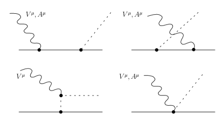
The background of the Born terms contains both vector current and axial vector current contributions. Since we neglect the strangeness of the nucleon, the weak vector current differs from the electromagnetic current only by a coupling constant. Accordingly, we have to calculate the Feynman diagrams of Fig. 3. While all diagrams contribute to the vector current, the pion pole diagram does not contribute to the axial current. For the calculation of the Feynman diagrams we use the following interaction Lagrangians

$${\cal L}_{\pi NN}^{PV} = \frac{f_{\pi NN}}{m_{\pi}}\bar{\psi}\gamma_{\mu}\gamma_{5}\vec{\tau}\psi\cdot\partial^{\mu}\vec{\phi}\,,$$ (33)

$${\cal L}_{V^{\mu}NN} = -e\,\bar{\psi}\frac{1}{2}\bigg{[}(\xi_{V}^{I=0}F_{1}^{s}+\xi_{V}^{I=1}\tau_{3}F_{1}^{v})\gamma_{\mu}V^{\mu}-(\xi_{V}^{I=0}\kappa_{s}F_{2}^{s}+\xi_{V}^{I=1}\kappa_{v}\tau_{3}F_{2}^{v})\frac{\sigma_{\mu\nu}}{2m}\partial^{\nu}V^{\mu}\bigg{]}\psi\,,$$ (34)

$${\cal L}_{V^{\mu}\pi\pi} = -e\,\xi_{V}^{I=1}F_{\pi}(\vec{\phi}\times\partial_{\mu}\vec{\phi})_{3}V^{\mu}\,,$$ (35)

$${\cal L}_{V^{\mu}NN\pi} = e\,\xi_{V}^{I=1}\frac{f_{\pi NN}}{g_{a}m_{\pi}}G_{A}\bar{\psi}(\vec{\tau}\times\vec{\phi})_{3}\gamma_{\mu}\gamma_{5}\psi\,V^{\mu},\,$$ (36)

$${\cal L}_{A^{\mu}NN} = -e\,\xi_{A}^{I=1}\bar{\psi}\left[G_{A}\gamma_{\mu}A^{\mu}+G_{P}\frac{i\partial_{\mu}}{2m}A^{\mu}\right]\gamma_{5}\frac{\tau_{3}}{2}\psi\,,$$ (37)

$${\cal L}_{A^{\mu}NN\pi} = e\,\xi_{A}^{I=1}\frac{f_{\pi NN}}{g_{a}m_{\pi}}\bar{\psi}(\vec{\tau}\times\vec{\phi})_{3}\left(F_{1}^{v}\gamma_{\mu}A^{\mu}-\kappa_{v}F_{2}^{v}\frac{\sigma_{\mu\nu}}{2m}\partial^{\nu}A^{\mu}\right)\psi\,,$$ (38)

with $\kappa_{(s,v)}=(\kappa_{p}\pm\kappa_{n})$. The isospin factors $\xi$ follow from the decomposition of the corresponding quark current operators according to strong isospin [14]. For the electromagnetic current these factors are equal to unity, for the weak neutral current we have

$$\xi_{V}^{I=1} = \frac{1}{2\sin\theta_{W}\cos\theta_{W}}(1-2\sin^{2}\theta_{W})\,,$$ (39)

$$\xi_{V}^{I=0} = -\frac{1}{2\sin\theta_{W}\cos\theta_{W}}2\sin^{2}\theta_{W}\,,$$ (40)

$$\xi_{A}^{I=1} = -\frac{1}{2\sin\theta_{W}\cos\theta_{W}}\,.$$ (41)

Note that there appears no isoscalar contribution to the axial vector current, i.e. $\xi_{A}^{I=0}=0$, because strange quarks have been neglected. The form factors $F_{1}$, $F_{2}$, $F_{\pi}$, $G_{A}$ and $G_{P}$ are functions of momentum transfer $q^{2}$. Since our calculation will be performed at relatively small momentum transfer, we have used simple dipole forms for the Sachs form factors, with the assumption $G_{A}/g_{a}=F_{\pi}=F_{1}^{v}$. This insures gauge invariance without additional gauge terms. With standard methods and neglecting the lepton mass terms, we obtain the invariant matrix elements

$${\cal M}_{s} = \xi_{V}^{I=1}\frac{f_{\pi NN}}{m_{\pi}}\bar{u}(\vec{P_{f}})\bigg{[}\gamma_{5}/\!\!\!k_{\pi}\frac{/\!\!\!\!\!\,P_{i}+/\!\!\!q+m}{s-m^{2}}\left(\tilde{I}_{s}^{D}/\!\!\!\epsilon+i\tilde{I}_{s}^{P}\frac{\sigma_{\mu\nu}}{2m}q^{\nu}\epsilon^{\mu}\right)\bigg{]}u(\vec{P_{i}})\,,$$ (42)

$${\cal M}_{u} = \xi_{V}^{I=1}\frac{f_{\pi NN}}{m_{\pi}}\bar{u}(\vec{P_{f}})\bigg{[}\left(\tilde{I}_{u}^{D}/\!\!\!\epsilon+i\tilde{I}_{u}^{P}\frac{\sigma_{\mu\nu}}{2m}q^{\nu}\epsilon^{\mu}\right)\frac{/\!\!\!\!\!\,P_{i}-/\!\!\!k_{\pi}+m}{u-m^{2}}\gamma_{5}/\!\!\!k_{\pi}\bigg{]}u(\vec{P_{i}})\,,$$ (43)

$${\cal M}_{t} = \xi_{V}^{I=1}\frac{f_{\pi NN}}{m_{\pi}}\frac{\epsilon\cdot(2k_{\pi}-q)}{t-m_{\pi}^{2}}2mI_{t}F_{\pi}\bar{u}(\vec{P_{f}})\gamma_{5}u(\vec{P_{i}})\,,$$ (44)

$${\cal M}_{c} = \xi_{V}^{I=1}\frac{f_{\pi NN}}{g_{a}m_{\pi}}I_{t}G_{A}\bar{u}(\vec{P_{f}})/\!\!\!\epsilon\gamma_{5}u(\vec{P_{i}})\,,$$ (45)

$${\cal M}_{s}^{5} = -\xi_{A}^{I=1}\frac{f_{\pi NN}}{m_{\pi}}\bar{u}(\vec{P_{f}})\left[/\!\!\!k_{\pi}\frac{/\!\!\!\!\!\,P_{i}+/\!\!\!q-m}{s-m^{2}}\tilde{I}_{s}^{A}/\!\!\!\epsilon\right]u(\vec{P_{i}})\,,$$ (46)

$${\cal M}_{u}^{5} = -\xi_{A}^{I=1}\frac{f_{\pi NN}}{m_{\pi}}\bar{u}(\vec{P_{f}})\left[\tilde{I}_{u}^{A}/\!\!\!\epsilon\frac{/\!\!\!\!\!\,P_{i}-/\!\!\!k_{\pi}-m}{u-m^{2}}/\!\!\!k_{\pi}\right]u(\vec{P_{i}})\,,$$ (47)

$${\cal M}_{c}^{5} = \xi_{A}^{I=1}\frac{f_{\pi NN}}{g_{a}m_{\pi}}I_{t}\bar{u}(\vec{P_{f}})\left[\gamma_{\mu}F_{1}^{v}+i\frac{F_{2}^{v}}{2m}\sigma_{\mu\nu}q^{\nu}\right]\epsilon^{\mu}u(\vec{P_{i}})\,.$$ (48)

Note that there do not appear any induced pseudoscalar terms, because the lepton mass terms have been neglected. The electromagnetic matrix element is the sum of the first 4 terms in (42), corresponding to s, u and t channel pole terms and the contact term(”c”). The matrix element of the weak neutral current is the corresponding sum of the combinations ${\cal M}+{\cal M}^{5}$. The following abbreviations for the isospin matrix elements have been used in (42):

$$I_{t} = I^{-},$$ (49)

$$\tilde{I}_{(s,u)}^{D} = \frac{1}{2}\left[\frac{\xi_{V}^{I=0}}{\xi_{V}^{I=1}}F_{1}^{s}I^{0}+F_{1}^{v}(I^{+}\pm I^{-})\right],$$ (50)

$$\tilde{I}_{(s,u)}^{P} = \frac{1}{2}\left[\frac{\xi_{V}^{I=0}}{\xi_{V}^{I=1}}F_{2}^{s}I^{0}+F_{2}^{v}(I^{+}\pm I^{-})\right],$$ (51)

$$\tilde{I}_{(s,u)}^{A} = \frac{1}{2}\left[G_{A}(I^{+}\pm I^{-})\right]\,,$$ (52)

with $I^{(\pm,0)}$ as defined in (13). The invariant amplitudes obtained from (42) are identical to the results of [15]. They can be found in Appendix B.

B Resonant contributions

In the kinematical region between threshold and about 400 MeV excitation energy, the dominant resonant contributions are due to the $\Delta(1232)$. We treat the $\Delta$ as a Rarita-Schwinger field and use the on-shell form of the propagator modified by a phenomenological constant width,

$$\Delta_{\mu\nu} = \frac{/\!\!\!p+M}{p^{2}-M^{2}+i\Gamma M}\left(g_{\mu\nu}-\frac{1}{3}\gamma_{\mu}\gamma_{\nu}-\frac{2p_{\mu}p_{\nu}}{3M^{2}}+\frac{p_{\mu}\gamma_{\nu}-\gamma_{\mu}p_{\nu}}{3M}\right)\,.$$ (53)

$M=1210\mbox{ MeV}$ is obtained as the real part of the $\Delta$ pole [21]. The width $\Gamma=85\mbox{ MeV}$ is fitted to the experimental data for pion electroproduction [16, 17], which is close to the imaginary part of the pole [21], $\Gamma=100\mbox{ MeV}$ . The Feynman diagrams to be calculated are shown in Fig. 4. We use the phenomenological $N\Delta$ transition currents [9]

$${J}_{\mu}^{EM} = \bar{u}^{\lambda}(\vec{p^{\prime}})\left[\left(\frac{C_{3}^{\gamma}}{m}\gamma^{\nu}+\frac{C_{4}^{\gamma}}{m^{2}}{p^{\prime}}^{\nu}+\frac{C_{5}^{\gamma}}{m^{2}}p^{\nu}\right)(g_{\lambda\mu}g_{\rho\nu}-g_{\lambda\rho}g_{\mu\nu})q^{\rho}\gamma_{5}\right]u(\vec{p})\,,$$ (54)

$${J}_{\mu}^{NC} = \bar{u}^{\lambda}(\vec{p^{\prime}})\left[\left(\frac{C_{3V}^{Z}}{m}\gamma^{\nu}+\frac{C_{4V}^{Z}}{m^{2}}{p^{\prime}}^{\nu}+\frac{C_{5V}^{Z}}{m^{2}}p^{\nu}\right)\vphantom{\frac{1}{2}}(g_{\lambda\mu}g_{\rho\nu}-g_{\lambda\rho}g_{\mu\nu})q^{\rho}\gamma_{5}+C_{6V}^{Z}g_{\lambda\mu}\gamma_{5}\right.$$ (56)

$$+\left.\left(\frac{C_{3A}^{Z}}{m}\gamma^{\nu}+\frac{C_{4A}^{Z}}{m^{2}}{p^{\prime}}^{\nu}\right)(g_{\lambda\mu}g_{\rho\nu}-g_{\lambda\rho}g_{\mu\nu})q^{\rho}+C_{5A}^{Z}g_{\lambda\mu}+\frac{C_{6A}^{Z}}{m^{2}}p_{\lambda}q_{\mu}\right]u(\vec{p})\,.$$

The form factors $C_{3}$ to $C_{6}$ are taken from Nath et al.[9], with a $q^{2}$ dependence as in [22]. The $\pi N\Delta$ vertex has the effective form [23]

$$\Lambda^{\mu}_{\pi N\Delta}=\frac{f_{\pi N\Delta}}{m_{\pi}}k_{\pi}^{\mu}\,.$$ (57)

With (53)-(57) we obtain the invariant matrix elements for s channel $\Delta$ production,

$${\cal M}^{EM}_{s\Delta} = \frac{f_{\pi N\Delta}}{mm_{\pi}}\bar{u}(\vec{P_{f}})k^{\pi}_{\sigma}\Delta^{\sigma\lambda}\bigg{[}C_{3}^{\gamma}(q_{\lambda}\gamma_{\mu}-g_{\lambda\mu}/\!\!\!q)+\frac{C_{4}^{\gamma}}{m}(q_{\lambda}(P_{f}+k_{\pi})_{\mu}$$ (59)

$$-q\cdot(P_{f}+k_{\pi})g_{\lambda\mu})\bigg{]}\gamma_{5}\epsilon^{\mu}u(\vec{P_{i}})\,,$$

$${\cal M}^{NC}_{s\Delta} = \xi_{V}^{I=1}{\cal M}^{EM}_{s\Delta}\vphantom{\frac{1}{2}},$$ (60)

$${\cal M}^{5NC}_{s\Delta} = -\xi_{A}^{I=1}\frac{f_{\pi N\Delta}}{mm_{\pi}}\bar{u}(\vec{P_{f}})k^{\pi}_{\sigma}\Delta^{\sigma\lambda}\bigg{[}C_{3}^{A}(q_{\lambda}\gamma_{\mu}-g_{\lambda\mu}/\!\!\!q)+\frac{C_{4}^{A}}{m}(q_{\lambda}(P_{f}+k_{\pi})_{\mu}$$ (62)

$$-q\cdot(P_{f}+k_{\pi})g_{\lambda\mu})-C_{5}^{A}mg_{\lambda\mu}\bigg{]}\epsilon^{\mu}u(\vec{P_{i}})\,.$$

The corresponding u channel amplitudes are constructed by using the crossing properties of the invariant amplitudes (18). These invariant matrix elements can now be decomposed into invariant amplitudes as in (14). The result of this calculation is listed in Appendix C.

IV Results

As a first test of the model we have calculated the inclusive electromagnetic cross section. The experimental data for this process [16, 17] could be reproduced within about 5% over the whole energy region from threshold to about 400 MeV excitation energy.

Fig. 5 shows the asymmetry for the proton and the neutron in various kinematical situations. The two upper figures compare the asymmetry for proton and neutron as function of the photon equivalent energy,

$$k_{\gamma}=(W^{2}-m^{2})/2m\,,$$ (63)

the lab energy necessary to excite a hadronic system with cm energy W. At small excitation energies the asymmetry is essentially given by background contributions, whereas the $\Delta$ resonance dominates at the higher energies. While the individual contributions vary strongly, the coherent sum is essentially constant. In particular, the resonance structure of the inclusive cross sections is essentially wiped out when the asymmetries are calculated. As demonstrated in the two lower figures of Fig. 5, this effect is quite independent of the kinematics except for a trivial dependence on the momentum transfer. For the proton this $Q^{2}$ dependence is well described by the simple estimate

$$A\approx-\frac{G_{F}Q^{2}}{e^{2}}\approx-10^{-4}Q^{2}/\mbox{ GeV}^{2}\;,$$ (64)

where $G_{F}$ is the Fermi coupling constant. In the case of the neutron, the asymmetry is somewhat smaller, at about 80% of the proton case, showing a slight enhancement in the resonance peak.

In Fig. 6 the asymmetry is shown at an incident electron energy of $\epsilon_{i}=800\mbox{ MeV}$ and at $W=1232\mbox{ MeV}$, directly in the resonance peak. In this kinematical situation, the asymmetry is strongly dominated by the $\Delta$, the background contributions cancel against the interference terms (upper panel). Therefore, the neglect of background terms as in the work of Nath et al.[9] is well justified. As is shown in the lower panel of this figure, we are able to reproduce those results except for an overall scaling factor of about 90 %. In the work of Cahn et al.[11] the vector coupling between the $Z^{0}$ and the electron has been neglected. This corresponds to $\sin^{2}\theta_{W}=1/4$ and produces a somewhat lower curve with a flat distribution in $Q^{2}$. We have also compared our calculation to the results of Li et al. [13] and find a reasonable agreement. However, the calculation of Ishankuliev et al. [12] disagrees with all others by a factor $1/2$ seemingly due to a wrong coupling constant.

Preliminary studies of the $\pi N$ $\sigma$-term (22) have shown only small effects of this physically interesting quantity on the asymmetry. Unfortunately, the coupling of the $Z^{0}$ to the axial current of the hadron appears together with the vector coupling to the electron which is strongly suppressed by the value of the Weinberg angle. In addition, the $S$-wave multipole ${\cal L}_{0+}$ contributes to the asymmetry only by interference with the electromagnetic $P$-waves. In the usual conventions this contribution is proportional to $(2M_{1+}+M_{1-}){\cal L}_{0+}$. As a consequence, the multipole ${\cal L}_{0+}$ is further suppressed near threshold.

V Summary and Conclusions

The aim of this work has been to investigate parity violating (PV) contributions to pion electroproduction. Only PV effects due to interference between $\gamma$ and $Z^{0}$ exchange have been considered. PV effects in the strong interaction, as discussed by Li et al.[13], have been neglected. The appropriate observable to study these effects is the asymmetry defined in (1). A simple phenomenological model with effective Lagrangian densities has been constructed that allows for the calculation of the asymmetry in the kinematical region from pion threshold to $\Delta(1232)$ resonance. The model is fully relativistic, fulfils the crossing symmetry and is gauge invariant due to our simple choice of the form factors. The invariant amplitudes for the nonresonant contributions respect PCAC. The $\Delta$ resonance is treated as a Rarita-Schwinger field with phenomenological transition currents. For the propagator, the on-shell form with the $\Delta$ pole of the $\pi N$ scattering matrix is used. The nonresonant contributions are created by the usual pseudovector $\pi N$ coupling and phenomenological transition currents. The weak neutral vector current is traced back to the electromagnetic one by decomposing the quark currents according to strong isospin. For the axial current, a contact term has been introduced in addition to the $s$ and $u$ channel nucleon Born terms. This contact term is necessary to fulfil the low energy theorem of Adler [15] for the nonresonant contributions.

The calculated asymmetry is nearly constant as function of excitation energy. It increases linearly with the square of the four-momentum transfer, $A\approx 10^{-4}q^{2}/\mbox{GeV}^{2}$ for the proton, and has about 80% of that value for the neutron. Previous calculations for the excitation of the $\Delta$ isobar could be reproduced reasonably well, while our results are at variance with some of the earlier work on the background contributions.

In conclusion we find the following results:

• The asymmetry grows linearly with the momentum transfer $Q^{2}$ and is nearly independent of the excitation energy.

• The expected asymmetries for pion electroproduction are comparable with the asymmetries found for elastic electron scattering.

• Because of the value of the Weinberg angle, the vector coupling of the $Z^{0}$ at the electron vertex is suppressed. As a consequence, the asymmetry is dominated by the hadronic vector current, the contributions of the hadronic axial currents being of the order of 10 - 20 % only.

• A precision measurement of the asymmetries is potentially an independent experiment to determine the important $\pi N$ $\sigma$-term, which appears in the $S$-wave multipole ${\cal L}_{0+}$ of the hadronic axial current. Unfortunately, the $\sigma$-term will be difficult to measure, because the hadronic axial current is suppressed and furthermore, the multipole ${\cal L}_{0+}$ appears in the asymmetry only by its interference with $P$-wave multipoles.

Finally, we would like to comment on some possible improvements of the calculations:

• The simple superposition of Born and resonance terms violates the Watson theorem. It would be necessary to perform a multipole decomposition and to unitarize at least the multipoles carrying the phase of the $\Delta(3,3)$ resonance.

• We have neglected the contribution of the strange sea to the hadronic transition currents. Taking account of such effects would require additional, as yet undetermined form factors. However, it is unlikely that pion production would be strongly modified by strangeness degrees of freedom.

• Though we have not found large contributions of the $\sigma$-term to the asymmetry, this matter deserves more systematical studies. Clearly, any further independent measurement of this important quantity would be invaluable.

A Structure Functions

The amplitudes $V_{i}$ for the electromagnetic current and $\tilde{V_{i}},\tilde{A_{i}}$ for the weak neutral current have the following isospin decomposition for Born terms and $\Delta$ contributions:

$$V_{i} = I^{0}V_{i}^{0}+I^{+}(V_{i}^{+}+V_{i,\Delta}^{+})+I^{-}(V_{i}^{-}+V_{i,\Delta}^{-})\,,$$ (A1)

$$\tilde{V}_{i} = I^{0}\tilde{V}_{i}^{0}+I^{+}(\tilde{V}_{i}^{+}+\tilde{V}_{i,\Delta}^{+})+I^{-}(\tilde{V}_{i}^{-}+\tilde{V}_{i,\Delta}^{-})\,,$$ (A2)

$$\tilde{A}_{i} = I^{+}(\tilde{A}_{i}^{+}+\tilde{A}_{i,\Delta}^{+})+I^{-}(\tilde{A}_{i}^{-}+\tilde{A}_{i,\Delta}^{-})\,.$$ (A3)

Structure functions for the interference tensor

Symmetric part

$$W_{1}^{I} = {\mathrm{Re}}(V_{1}^{*}\tilde{V}_{1})\left(4m^{2}(\nu^{2}-\nu_{B}^{2})+m_{\pi}^{2}q^{2}\right)+{\mathrm{Re}}(V_{3}^{*}\tilde{V}_{3})4m^{2}\nu_{B}^{2}\left(4m^{2}-(4m\nu_{B}+m_{\pi}^{2}+q^{2})\right)$$ (A4)

$$+ {\mathrm{Re}}(V_{4}^{*}\tilde{V}_{4})4m^{2}\left(m_{\pi}^{2}q^{2}-4m^{2}\nu_{B}^{2}-\nu^{2}(4m\nu_{B}+m_{\pi}^{2}+q^{2})\right)$$ (A5)

$$+ {\mathrm{Re}}(V_{6}^{*}\tilde{V}_{6})q^{4}\left(4m^{2}-(4m\nu_{B}+m_{\pi}^{2}+q^{2})\right)-({\mathrm{Re}}(V_{1}^{*}\tilde{V}_{3})+{\mathrm{Re}}(V_{3}^{*}\tilde{V}_{1}))8m^{3}\nu\nu_{B}$$ (A6)

$$+ ({\mathrm{Re}}(V_{1}^{*}\tilde{V}_{4})+(V_{4}^{*}\tilde{V}_{1}))2m\left(4m^{2}\nu_{B}^{2}-m_{\pi}^{2}q^{2}\right)-({\mathrm{Re}}(V_{1}^{*}\tilde{V}_{6})+{\mathrm{Re}}(V_{6}^{*}\tilde{V}_{1}))4m^{2}q^{2}\nu$$ (A7)

$$+ ({\mathrm{Re}}(V_{3}^{*}\tilde{V}_{4})+{\mathrm{Re}}(V_{4}^{*}\tilde{V}_{3}))4m^{2}\nu\nu_{B}(4m\nu_{B}+m_{\pi}^{2}+q^{2})$$ (A8)

$$+ ({\mathrm{Re}}(V_{3}^{*}\tilde{V}_{6})+{\mathrm{Re}}(V_{6}^{*}\tilde{V}_{3}))2m\nu_{B}q^{2}\left(4m^{2}-(4m\nu_{B}+m_{\pi}^{2}+q^{2})\right)$$ (A9)

$$+ ({\mathrm{Re}}(V_{4}^{*}\tilde{V}_{6})+{\mathrm{Re}}(V_{6}^{*}\tilde{V}_{4}))2m\nu q^{2}(4m\nu_{B}+m_{\pi}^{2}+q^{2})$$ (A10)

$$W_{2}^{I} = -4m^{2}\big{[}{\mathrm{Re}}(V_{1}^{*}\tilde{V}_{1})q^{2}+{\mathrm{Re}}(V_{2}^{*}\tilde{V}_{2})4m^{2}\nu_{B}^{2}(4m\nu_{B}+m_{\pi}^{2}+q^{2})$$ (A12)

$$- {\mathrm{Re}}(V_{3}^{*}\tilde{V}_{3})4m^{2}\nu_{B}^{2}+{\mathrm{Re}}(V_{4}^{*}\tilde{V}_{4})\left(4m^{2}\nu_{B}^{2}-m_{\pi}^{2}q^{2}\right)-{\mathrm{Re}}(V_{6}^{*}\tilde{V}_{6})q^{4}$$ (A13)

$$+ ({\mathrm{Re}}(V_{1}^{*}\tilde{V}_{2})+{\mathrm{Re}}(V_{2}^{*}\tilde{V}_{1}))2m\nu_{B}(q^{2}+2m\nu_{B})-({\mathrm{Re}}(V_{3}^{*}\tilde{V}_{6})+{\mathrm{Re}}(V_{6}^{*}\tilde{V}_{3}))2m\nu_{B}q^{2}\big{]}$$ (A14)

$$W_{3}^{I} = -m^{2}\big{[}{\mathrm{Re}}(V_{2}^{*}\tilde{V}_{2})(\nu_{B}-\nu)^{2}(4m\nu_{B}+m_{\pi}^{2}+q^{2})$$ (A16)

$$- {\mathrm{Re}}(V_{3}^{*}\tilde{V}_{3})(4m^{2}(\nu_{B}-\nu)^{2}+q^{2}(4m\nu_{B}+m_{\pi}^{2}-4m^{2}))$$ (A17)

$$+ {\mathrm{Re}}(V_{4}^{*}\tilde{V}_{4})(4m^{2}(\nu_{B}-\nu)^{2}-q^{2}(4m\nu+m_{\pi}^{2}4m^{2}))+{\mathrm{Re}}(V_{5}^{*}\tilde{V}_{5})q^{4}(4m\nu_{B}+m_{\pi}^{2}+q^{2})$$ (A18)

$$+ ({\mathrm{Re}}(V_{1}^{*}\tilde{V}_{2})+{\mathrm{Re}}(V_{2}^{*}\tilde{V}_{1}))2m(2m(\nu_{B}-\nu)^{2}+q^{2}(\nu_{B}-\nu))$$ (A19)

$$- ({\mathrm{Re}}(V_{1}^{*}\tilde{V}_{3})+{\mathrm{Re}}(V_{3}^{*}\tilde{V}_{1}))2mq^{2}+({\mathrm{Re}}(V_{1}^{*}\tilde{V}_{4})+{\mathrm{Re}}(V_{4}^{*}\tilde{V}_{1}))2mq^{2}$$ (A20)

$$- ({\mathrm{Re}}(V_{1}^{*}\tilde{V}_{5})+{\mathrm{Re}}(V_{5}^{*}\tilde{V}_{1}))q^{2}(2m(\nu_{B}-\nu)+q^{2})-({\mathrm{Re}}(V_{2}^{*}\tilde{V}_{3})+{\mathrm{Re}}(V_{3}^{*}\tilde{V}_{2}))4m^{2}q^{2}(\nu_{B}-\nu)$$ (A21)

$$- ({\mathrm{Re}}(V_{2}^{*}\tilde{V}_{5})+{\mathrm{Re}}(V_{5}^{*}\tilde{V}_{2}))2mq^{2}(\nu_{B}-\nu)(4m\nu_{B}+m_{\pi}^{2}+q^{2})$$ (A22)

$$+ ({\mathrm{Re}}(V_{2}^{*}\tilde{V}_{6})+{\mathrm{Re}}(V_{6}^{*}\tilde{V}_{2}))4m^{2}q^{2}(\nu_{B}-\nu)+({\mathrm{Re}}(V_{3}^{*}\tilde{V}_{4})+{\mathrm{Re}}(V_{4}^{*}\tilde{V}_{3}))q^{2}(2m(\nu_{B}+\nu)+m_{\pi}^{2})$$ (A23)

$$+ ({\mathrm{Re}}(V_{3}^{*}\tilde{V}_{5})+{\mathrm{Re}}(V_{5}^{*}\tilde{V}_{3}))2mq^{4}-({\mathrm{Re}}(V_{3}^{*}\tilde{V}_{6})+{\mathrm{Re}}(V_{6}^{*}\tilde{V}_{3}))q^{2}(2m(\nu_{B}-\nu)+q^{2})$$ (A24)

$$+ ({\mathrm{Re}}(V_{4}^{*}\tilde{V}_{6})+{\mathrm{Re}}(V_{6}^{*}\tilde{V}_{4}))q^{2}(2m(\nu_{B}-\nu)+q^{2})-({\mathrm{Re}}(V_{5}^{*}\tilde{V}_{6})+{\mathrm{Re}}(V_{6}^{*}\tilde{V}_{5}))2mq^{4}\big{]}$$ (A25)

$$W_{4}^{I} = m^{2}\big{[}{\mathrm{Re}}(V_{1}^{*}\tilde{V}_{1})(4m\nu+m_{\pi}^{2}-q^{2})-{\mathrm{Re}}(V_{2}^{*}\tilde{V}_{2})4m^{2}\nu_{B}^{2}(4m\nu_{B}+m_{\pi}^{2}+q^{2})$$ (A27)

$$+ {\mathrm{Re}}(V_{4}^{*}\tilde{V}_{4})(4m^{2}(m_{\pi}^{2}-(\nu+\nu_{B})^{2})+m_{\pi}^{2}(q^{2}-4m\nu))-{\mathrm{Re}}(V_{5}^{*}\tilde{V}_{5})4m^{2}\nu_{B}^{2}(4m\nu_{B}+m_{\pi}^{2}+q^{2})$$ (A28)

$$+ {\mathrm{Re}}(V_{6}^{*}\tilde{V}_{6})(4m^{2}(q^{2}+\nu^{2}-\nu_{B}^{2})-q^{2}(4m(\nu+\nu_{B})+m_{\pi}^{2}))$$ (A29)

$$- ({\mathrm{Re}}(V_{1}^{*}\tilde{V}_{2})+{\mathrm{Re}}(V_{2}^{*}\tilde{V}_{1}))2m\nu_{B}(2m(\nu_{B}-\nu)+q^{2})-({\mathrm{Re}}(V_{1}^{*}\tilde{V}_{3})+{\mathrm{Re}}(V_{3}^{*}\tilde{V}_{1}))4m^{2}\nu_{B}$$ (A30)

$$- ({\mathrm{Re}}(V_{1}^{*}\tilde{V}_{4})+{\mathrm{Re}}(V_{4}^{*}\tilde{V}_{1}))2mm_{\pi}^{2}-({\mathrm{Re}}(V_{1}^{*}\tilde{V}_{5})+{\mathrm{Re}}(V_{5}^{*}\tilde{V}_{1}))2m\nu_{B}(2m(\nu_{B}-\nu)+q^{2})$$ (A31)

$$- ({\mathrm{Re}}(V_{1}^{*}\tilde{V}_{6})+{\mathrm{Re}}(V_{6}^{*}\tilde{V}_{1}))4m^{2}\nu-({\mathrm{Re}}(V_{2}^{*}\tilde{V}_{3})+{\mathrm{Re}}(V_{3}^{*}\tilde{V}_{2}))8m^{3}\nu_{B}^{2}$$ (A32)

$$- ({\mathrm{Re}}(V_{2}^{*}\tilde{V}_{5})+{\mathrm{Re}}(V_{5}^{*}\tilde{V}_{2}))4m^{2}\nu_{B}^{2}(4m\nu_{B}+m_{\pi}^{2}+q^{2})+({\mathrm{Re}}(V_{2}^{*}\tilde{V}_{6})+{\mathrm{Re}}(V_{6}^{*}\tilde{V}_{2}))8m^{3}\nu_{B}^{2}$$ (A33)

$$+ ({\mathrm{Re}}(V_{3}^{*}\tilde{V}_{4})+{\mathrm{Re}}(V_{4}^{*}\tilde{V}_{3}))2m\nu_{B}(2m(\nu_{B}-\nu)+m_{\pi}^{2})-({\mathrm{Re}}(V_{3}^{*}\tilde{V}_{5})+{\mathrm{Re}}(V_{5}^{*}\tilde{V}_{3}))8m^{3}\nu_{B}^{2}$$ (A34)

$$+ ({\mathrm{Re}}(V_{3}^{*}\tilde{V}_{6})+{\mathrm{Re}}(V_{6}^{*}\tilde{V}_{3}))2m\nu_{B}(4m^{2}-2m(\nu_{B}-\nu)-m_{\pi}^{2})$$ (A35)

$$+ ({\mathrm{Re}}(V_{4}^{*}\tilde{V}_{6})+{\mathrm{Re}}(V_{6}^{*}\tilde{V}_{4}))2m((2m\nu_{B}+q^{2})(\nu+\nu_{B})+\nu m_{\pi}^{2})$$ (A36)

$$+ ({\mathrm{Re}}(V_{5}^{*}\tilde{V}_{6})+{\mathrm{Re}}(V_{6}^{*}\tilde{V}_{5}))8m^{3}\nu_{B}^{2}\big{]}$$ (A37)

Antisymmetric part

$$W_{5}^{I} = -2m^{2}\big{[}{\mathrm{Re}}(V_{1}^{*}\tilde{A}_{1})m_{\pi}^{2}+{\mathrm{Re}}(V_{3}^{*}\tilde{A}_{4})2m^{2}\nu_{B}-{\mathrm{Re}}(V_{4}^{*}\tilde{A}_{1})2mm_{\pi}^{2}-{\mathrm{Re}}(V_{4}^{*}\tilde{A}_{4})2m^{2}\nu$$ (A38)

$$+ {\mathrm{Re}}(V_{6}^{*}\tilde{A}_{4})mq^{2}\big{]}$$ (A39)

$$W_{6}^{I} = 2m^{3}\big{[}{\mathrm{Re}}(V_{1}^{*}\tilde{A}_{1})2(\nu_{B}-\nu)+{\mathrm{Re}}(V_{3}^{*}\tilde{A}_{1})4m\nu_{B}-{\mathrm{Re}}(V_{3}^{*}\tilde{A}_{4})2m\nu_{B}-{\mathrm{Re}}(V_{4}^{*}\tilde{A}_{1})4m\nu_{B}$$ (A41)

$$+ {\mathrm{Re}}(V_{4}^{*}\tilde{A}_{4})2m\nu+{\mathrm{Re}}(V_{6}^{*}\tilde{A}_{1})2q^{2}-{\mathrm{Re}}(V_{6}^{*}\tilde{A}_{4})q^{2}\big{]}$$ (A42)

$$W_{7}^{I} = 2m^{3}\big{[}{\mathrm{Re}}(V_{1}^{*}\tilde{A}_{4})m+{\mathrm{Re}}(V_{3}^{*}\tilde{A}_{1})2m\nu_{B}-{\mathrm{Re}}(V_{4}^{*}\tilde{A}_{1})2m\nu-{\mathrm{Re}}(V_{4}^{*}\tilde{A}_{4})2m^{2}$$ (A44)

$$+ {\mathrm{Re}}(V_{6}^{*}\tilde{A}_{4})q^{2}\big{]}$$ (A45)

$$W_{8}^{I} = 0$$ (A47)

$$W_{9}^{I} = 2m^{4}\big{[}{\mathrm{Re}}(V_{1}^{*}\tilde{A}_{1})-{\mathrm{Re}}(V_{1}^{*}\tilde{A}_{2})+{\mathrm{Re}}(V_{2}^{*}\tilde{A}_{1})2m\nu_{B}+{\mathrm{Re}}(V_{3}^{*}\tilde{A}_{5})2m\nu_{B}$$ (A49)

$$+ {\mathrm{Re}}(V_{4}^{*}\tilde{A}_{2})2m-{\mathrm{Re}}(V_{4}^{*}\tilde{A}_{4})m-{\mathrm{Re}}(V_{4}^{*}\tilde{A}_{5})2m\nu+{\mathrm{Re}}(V_{6}^{*}\tilde{A}_{5})q^{2}\big{]}$$ (A50)

$$W_{10}^{I} = -m^{4}\big{[}-{\mathrm{Re}}(V_{1}^{*}\tilde{A}_{1})-{\mathrm{Re}}(V_{1}^{*}\tilde{A}_{2})+{\mathrm{Re}}(V_{1}^{*}\tilde{A}_{3})+{\mathrm{Re}}(V_{2}^{*}\tilde{A}_{1})2m(\nu_{B}-\nu)$$ (A52)

$$- {\mathrm{Re}}(V_{3}^{*}\tilde{A}_{1})2m+{\mathrm{Re}}(V_{3}^{*}\tilde{A}_{4})m+{\mathrm{Re}}(V_{3}^{*}\tilde{A}_{5})2m\nu_{B}-{\mathrm{Re}}(V_{3}^{*}\tilde{A}_{6})2m\nu_{B}$$ (A53)

$$+ {\mathrm{Re}}(V_{4}^{*}\tilde{A}_{1})4m+{\mathrm{Re}}(V_{4}^{*}\tilde{A}_{2})2m-{\mathrm{Re}}(V_{4}^{*}\tilde{A}_{3})2m-{\mathrm{Re}}(V_{4}^{*}\tilde{A}_{4})m$$ (A54)

$$- {\mathrm{Re}}(V_{4}^{*}\tilde{A}_{5})2m\nu+{\mathrm{Re}}(V_{4}^{*}\tilde{A}_{6})2m\nu-{\mathrm{Re}}(V_{5}^{*}\tilde{A}_{1})q^{2}+{\mathrm{Re}}(V_{6}^{*}\tilde{A}_{5})q^{2}$$ (A55)

$$- {\mathrm{Re}}(V_{6}^{*}\tilde{A}_{6})q^{2}\big{]}$$ (A56)

Structure functions for the electromagnetic tensor

The structure functions for the electromagnetic tensor follow from (A4) via the substitutions

$${\mathrm{Re}}(V_{k}^{*}\tilde{V}_{k}) \rightarrow |V_{k}|^{2}\,,$$ (A57)

$$({\mathrm{Re}}(V_{l}^{*}\tilde{V}_{k})+{\mathrm{Re}}(V_{k}^{*}\tilde{V}_{l})) \rightarrow 2{\mathrm{Re}}(V_{l}^{*}V_{k})\,,\qquad\forall l,k=1\ldots 6\,.$$ (A58)

B Invariant Amplitudes for the Nonresonant Contributions

Vector currents

$$V_{1}^{(0,+)} = i\frac{f_{\pi NN}}{2m_{\pi}}\left(F_{1}^{(s,v)}\left(\frac{1}{\nu-\nu_{B}}-\frac{1}{\nu+\nu_{B}}\right)+\frac{F_{2}^{(s,v)}}{m}\right)$$ (B1)

$$V_{2}^{(0,+)} = i\frac{f_{\pi NN}}{2m_{\pi}}\left(-\frac{F_{1}^{(s,v)}}{2m\nu_{B}}\left(\frac{1}{\nu-\nu_{B}}-\frac{1}{\nu+\nu_{B}}\right)\right)$$ (B2)

$$V_{3}^{(0,+)} = i\frac{f_{\pi NN}}{2m_{\pi}}\left(-\frac{F_{2}^{(s,v)}}{2m}\left(\frac{1}{\nu-\nu_{B}}+\frac{1}{\nu+\nu_{B}}\right)\right)$$ (B3)

$$V_{4}^{(0,+)} = i\frac{f_{\pi NN}}{2m_{\pi}}\left(-\frac{F_{2}^{(s,v)}}{2m}\left(\frac{1}{\nu-\nu_{B}}-\frac{1}{\nu+\nu_{B}}\right)\right)$$ (B4)

$$V_{5}^{(0,+)} = V_{6}^{(0,+)}=0$$ (B5)

$$V_{1}^{(-)} = i\frac{f_{\pi NN}}{2m_{\pi}}\left(F_{1}^{v}\left(\frac{1}{\nu-\nu_{B}}+\frac{1}{\nu+\nu_{B}}\right)\right)$$ (B7)

$$V_{2}^{(-)} = i\frac{f_{\pi NN}}{2m_{\pi}}\left(-\frac{F_{1}^{v}}{2m\nu_{B}}\left(\frac{1}{\nu-\nu_{B}}+\frac{1}{\nu+\nu_{B}}\right)\right)$$ (B8)

$$V_{3}^{(-)} = i\frac{f_{\pi NN}}{2m_{\pi}}\left(-\frac{F_{2}^{v}}{2m}\left(\frac{1}{\nu-\nu_{B}}-\frac{1}{\nu+\nu_{B}}\right)\right)$$ (B9)

$$V_{4}^{(-)} = i\frac{f_{\pi NN}}{2m_{\pi}}\left(-\frac{F_{2}^{v}}{2m}\left(\frac{1}{\nu-\nu_{B}}+\frac{1}{\nu+\nu_{B}}\right)\right)$$ (B10)

$$V_{5}^{(-)} = i\frac{f_{\pi NN}}{2m_{\pi}}\left(\frac{2F_{1}^{v}}{\nu_{B}\left(q^{2}+4m\nu_{B}\right)}\right)$$ (B11)

$$V_{6}^{(-)} = 0$$ (B12)

The amplitudes $\tilde{V}_{j}^{(\pm,0)}$ for the neutral weak vector current follow from

$$\tilde{V}_{j}^{(\pm)} = \xi_{V}^{I=1}V_{j}^{(\pm)},\qquad j=1,\ldots,6\,$$ (B13)

$$\tilde{V}_{j}^{(0)} = \xi_{V}^{I=0}V_{j}^{(0)},\qquad j=1,\ldots,6\;.$$ (B14)

Axial currents

$$A_{1}^{(+)} = i\frac{f_{\pi NN}}{2m_{\pi}}\left(G_{A}\left(\frac{1}{\nu-\nu_{B}}+\frac{1}{\nu+\nu_{B}}\right)\right)$$ (B15)

$$A_{3}^{(+)} = i\frac{f_{\pi NN}}{2m_{\pi}}\left(G_{A}\left(\frac{1}{\nu-\nu_{B}}-\frac{1}{\nu+\nu_{B}}\right)\right)$$ (B16)

$$A_{2}^{(+)} = A_{4}^{(+)}=A_{5}^{(+)}=A_{6}^{(+)}=A_{7}^{(+)}=A_{8}^{(+)}=0$$ (B17)

$$A_{1}^{(-)} = i\frac{f_{\pi NN}}{2m_{\pi}}\left(G_{A}\left(\frac{1}{\nu-\nu_{B}}-\frac{1}{\nu+\nu_{B}}\right)+\frac{F_{2}^{v}}{mg_{a}}\right)$$ (B19)

$$A_{2}^{(-)} = i\frac{f_{\pi NN}}{2m_{\pi}}\left(-\frac{F_{2}^{v}}{mg_{a}}\right)$$ (B20)

$$A_{3}^{(-)} = i\frac{f_{\pi NN}}{2m_{\pi}}\left(G_{A}\left(\frac{1}{\nu-\nu_{B}}+\frac{1}{\nu+\nu_{B}}\right)\right)$$ (B21)

$$A_{4}^{(-)} = i\frac{f_{\pi NN}}{2m_{\pi}}\left(-\frac{2}{m}G_{A}+(F_{1}^{v}+F_{2}^{v})\frac{2}{mg_{a}}\right)$$ (B22)

$$A_{5}^{(-)} = A_{6}^{(-)}=A_{7}^{(-)}=A_{8}^{(-)}=0$$ (B23)

The amplitudes $\tilde{A}_{j}^{(\pm)}$ for the neutral weak axial current follow from

$$\tilde{A}_{j}^{(\pm)} = \xi_{A}^{I=1}A_{j}^{(\pm)},\qquad j=1,\ldots,8\,.$$ (B24)

C Invariant Amplitudes for the Resonant Contributions

In the following, we give the s channel contributions of the resonance. The corresponding u channel contributions may be obtained by crossing symmetry, see (18).

Vector currents

$$V_{1,\Delta}^{s} = i\frac{f_{\pi N\Delta}}{mm_{\pi}}\frac{1}{s-m_{\Delta}^{2}+i\Gamma m_{\Delta}}\bigg{[}C_{3}^{\gamma}\bigg{(}-2m\nu_{B}-\frac{2}{3}m_{\pi}^{2}-\frac{2}{3m_{\Delta}^{2}}(m(\nu-\nu_{B})+\frac{m_{\pi}^{2}}{2})$$ (C4)

$$(m(\nu-\nu_{B})+m(m+m_{\Delta})+\frac{q^{2}}{2})+\frac{1}{3m_{\Delta}}((m(\nu-\nu_{B})-\frac{q^{2}}{2})(m+m_{\Delta})-mm_{\pi}^{2})\bigg{)}$$

$$-\frac{C_{4}^{\gamma}}{m}\bigg{(}-2m^{2}\nu_{B}-\frac{1}{3}((m+m_{\Delta})(m(\nu-\nu_{B})+\frac{q^{2}}{2})+mm_{\pi}^{2})$$

$$+\frac{1}{3m_{\Delta}}(m(\nu-\nu_{B})+\frac{m_{\pi}^{2}}{2})(m(\nu-\nu_{B})+m(m+m_{\Delta})+\frac{q^{2}}{2})\bigg{)}\Bigg{]}$$

$$V_{2,\Delta}^{s} = i\frac{f_{\pi N\Delta}}{mm_{\pi}}\frac{1}{s-m_{\Delta}^{2}+i\Gamma m_{\Delta}}\bigg{[}C_{3}^{\gamma}\bigg{(}1+\frac{2}{3m_{\Delta}^{2}}\frac{1}{2}(m(\nu-\nu_{B})+\frac{m_{\pi}^{2}}{2})\frac{q^{2}}{2m\nu_{B}}$$ (C7)

$$+\frac{1}{2}\frac{1}{3m_{\Delta}}(m+m_{\Delta})\frac{q^{2}}{2m\nu_{B}}\bigg{)}-\frac{C_{4}^{\gamma}}{m}\bigg{(}\frac{(m_{\Delta}-m)}{2}+\frac{1}{6}(m+m_{\Delta})\frac{q^{2}}{2m\nu_{B}}$$

$$-\frac{1}{3m_{\Delta}}(m(\nu-\nu_{B})+\frac{m_{\pi}^{2}}{2})\frac{1}{2}\frac{q^{2}}{2m\nu_{B}}\bigg{)}\bigg{]}$$

$$V_{3,\Delta}^{s} = i\frac{f_{\pi N\Delta}}{mm_{\pi}}\frac{1}{s-m_{\Delta}^{2}+i\Gamma m_{\Delta}}\bigg{[}C_{3}^{\gamma}\bigg{(}\frac{(m+m_{\Delta})}{3}-\frac{2}{3m_{\Delta}^{2}}(m(\nu-\nu_{B})+\frac{m_{\pi}^{2}}{2})$$ (C10)

$$\frac{1}{2}(m+m_{\Delta})+\frac{1}{3m_{\Delta}}(2m(\nu-\nu_{B})+\frac{m_{\pi}^{2}}{2})\bigg{)}-\frac{C_{4}^{\gamma}}{m}\bigg{(}-(\nu m+\frac{q^{2}}{2})-\frac{m_{\pi}^{2}}{6}$$

$$+\frac{1}{3m_{\Delta}}(m(\nu-\nu_{B})+\frac{m_{\pi}^{2}}{2})\frac{1}{2}(m+m_{\Delta})\bigg{)}\bigg{]}$$

$$V_{4,\Delta}^{s} = i\frac{f_{\pi N\Delta}}{mm_{\pi}}\frac{1}{s-m_{\Delta}^{2}+i\Gamma m_{\Delta}}\bigg{[}C_{3}^{\gamma}\bigg{(}-\frac{2}{3}(m+m_{\Delta})-\frac{2}{3m_{\Delta}^{2}}(m(\nu-\nu_{B})+\frac{m_{\pi}^{2}}{2})$$ (C13)

$$\frac{1}{2}(m+m_{\Delta})-\frac{1}{3m_{\Delta}}\frac{1}{2}m_{\pi}^{2}\bigg{)}-\frac{C_{4}^{\gamma}}{m}\bigg{(}-m\nu_{B}-\frac{1}{6}m_{\pi}^{2}+\frac{1}{3m_{\Delta}}(m(\nu-\nu_{B})+\frac{m_{\pi}^{2}}{2})$$

$$\frac{1}{2}(m+m_{\Delta})\bigg{)}\bigg{]}$$

$$V_{5,\Delta}^{s} = i\frac{f_{\pi N\Delta}}{mm_{\pi}}\frac{1}{s-m_{\Delta}^{2}+i\Gamma m_{\Delta}}\bigg{[}C_{3}^{\gamma}\bigg{(}\frac{1}{2}(1-\frac{\nu}{\nu_{B}})(\frac{2}{3m_{\Delta}^{2}}(m(\nu-\nu_{B})+\frac{m_{\pi}^{2}}{2})$$ (C16)

$$+\frac{1}{3m_{\Delta}}(m+m_{\Delta}))\bigg{)}-\frac{C_{4}^{\gamma}}{m}\bigg{(}-\frac{1}{2}(m_{\Delta}-m)+\frac{1}{2}(1-\frac{\nu}{\nu_{B}})$$

$$(\frac{(m+m_{\Delta})}{3}-\frac{1}{3m_{\Delta}}(m(\nu-\nu_{B})+\frac{m_{\pi}^{2}}{2}))\bigg{)}\bigg{]}$$

$$V_{6,\Delta}^{s} = i\frac{f_{\pi N\Delta}}{mm_{\pi}}\frac{1}{s-m_{\Delta}^{2}+i\Gamma m_{\Delta}}\bigg{[}C_{3}^{\gamma}\bigg{(}\frac{2}{3m_{\Delta}^{2}}(m(\nu-\nu_{B})+\frac{m_{\pi}^{2}}{2})\frac{1}{2}(m+m_{\Delta})$$ (C18)

$$+\frac{1}{3m_{\Delta}}\frac{m_{\pi}^{2}}{2}\bigg{)}-\frac{C_{4}^{\gamma}}{m}\bigg{(}m\nu_{B}+\frac{m_{\pi}^{2}}{6}-\frac{1}{3m_{\Delta}}(m(\nu-\nu_{B})+\frac{m_{\pi}^{2}}{2})\frac{1}{2}(m+m_{\Delta})\bigg{)}\bigg{]}$$

The amplitudes $V_{j,\Delta}^{(\pm)}$ are calculated via

$$V_{j,\Delta}^{+} = \frac{2}{3}(V_{j,\Delta}^{s}+V_{j,\Delta}^{u})\,,$$ (C19)

$$V_{j,\Delta}^{-} = -\frac{1}{3}(V_{j,\Delta}^{s}-V_{j,\Delta}^{u})\,,\qquad j=1,\ldots,6\;,$$ (C20)

and the $\tilde{V}_{j,\Delta}^{(\pm)}$ for the neutral weak vector current follow from

$$\tilde{V}_{j,\Delta}^{(\pm)}=\xi_{V}^{I=1}V_{j,\Delta}^{(\pm)}\,,\qquad j=1,\ldots,6\;.$$ (C21)

Axial currents

$$A_{1,\Delta}^{s} = -i\frac{f_{\pi N\Delta}}{mm_{\pi}}\frac{1}{s-m_{\Delta}^{2}+i\Gamma m_{\Delta}}\bigg{[}\frac{C_{4}^{A}}{m}\bigg{(}\frac{1}{2}(m+m_{\Delta})(m(\nu-\nu_{B})+\frac{q^{2}}{2})$$ (C24)

$$-\frac{1}{3m_{\Delta}}(m(\nu-\nu_{B})+\frac{m_{\pi}^{2}}{2})(m(\nu-\nu_{B})+\frac{q^{2}}{2})\bigg{)}-C_{5}^{A}m\bigg{(}-\frac{1}{2}(m+m_{\Delta})$$

$$+\frac{1}{3m_{\Delta}}(m(\nu-\nu_{B})+\frac{m_{\pi}^{2}}{2})\bigg{)}\bigg{]}$$

$$A_{2,\Delta}^{s} = -i\frac{f_{\pi N\Delta}}{mm_{\pi}}\frac{1}{s-m_{\Delta}^{2}+i\Gamma m_{\Delta}}\bigg{[}\frac{C_{4}^{A}}{m}\bigg{(}-m\nu_{B}(m+m_{\Delta})-\frac{1}{3}(m+m_{\Delta})m(\nu-\nu_{B})$$ (C27)

$$+\frac{1}{3m_{\Delta}}(m(\nu-\nu_{B})+\frac{m_{\pi}^{2}}{2})m(\nu-\nu_{B})\bigg{)}-C_{5}^{A}m\bigg{(}-\frac{2}{3m_{\Delta}^{2}}(m(\nu-\nu_{B})+\frac{m_{\pi}^{2}}{2})$$

$$\frac{1}{2}(m+m_{\Delta})-\frac{1}{2}\frac{1}{3m_{\Delta}}m_{\pi}^{2}\bigg{)}\bigg{]}$$

$$A_{3,\Delta}^{s} = -i\frac{f_{\pi N\Delta}}{mm_{\pi}}\frac{1}{s-m_{\Delta}^{2}+i\Gamma m_{\Delta}}\bigg{[}\frac{C_{4}^{A}}{m}\bigg{(}-(m+m_{\Delta})(m\nu+\frac{q^{2}}{2})+\frac{1}{6}(m+m_{\Delta})q^{2}$$ (C30)

$$-\frac{1}{3m_{\Delta}}(m(\nu-\nu_{B})+\frac{m_{\pi}^{2}}{2})\frac{q^{2}}{2}\bigg{)}-C_{5}^{A}m\bigg{(}\frac{2}{3}(m+m_{\Delta})-\frac{2}{3m_{\Delta}^{2}}(m(\nu-\nu_{B})+m_{\pi}^{2})$$

$$\frac{1}{2}(m+m_{\Delta})+\frac{1}{3m_{\Delta}}m(\nu-\nu_{B})\bigg{)}\bigg{]}$$

$$A_{4,\Delta}^{s} = -i\frac{f_{\pi N\Delta}}{mm_{\pi}}\frac{1}{s-m_{\Delta}^{2}+i\Gamma m_{\Delta}}\bigg{[}\frac{C_{4}^{A}}{m}\bigg{(}\frac{m_{\pi}^{2}}{3m}(m(\nu-\nu_{B})+\frac{q^{2}}{2})-\frac{1}{3m_{\Delta}}(m(\nu-\nu_{B})$$ (C33)

$$+\frac{m_{\pi}^{2}}{2})(m(\nu-\nu_{B})+\frac{q^{2}}{2})\frac{(m+m_{\Delta})}{m}\bigg{)}-C_{5}^{A}m\bigg{(}-\frac{m_{\pi}^{2}}{3m}+\frac{1}{3m_{\Delta}}\frac{(m+m_{\Delta})}{m}$$

$$(m(\nu-\nu_{B})+\frac{m_{\pi}^{2}}{2})\bigg{)}\bigg{]}$$

$$A_{5,\Delta}^{s} = -i\frac{f_{\pi N\Delta}}{mm_{\pi}}\frac{1}{s-m_{\Delta}^{2}+i\Gamma m_{\Delta}}\bigg{[}\frac{C_{4}^{A}}{m}\bigg{(}m\nu_{B}-\frac{1}{6}(2m(m+m_{\Delta})-m_{\pi}^{2})$$ (C36)

$$-\frac{1}{2}\frac{1}{3m_{\Delta}}(m_{\Delta}-m)(m(\nu-\nu_{B})+\frac{m_{\pi}^{2}}{2})\bigg{)}-C_{5}^{A}m\bigg{(}\frac{1}{2}\frac{2}{3m_{\Delta}^{2}}(m(\nu-\nu_{B})+\frac{m_{\pi}^{2}}{2})$$

$$+\frac{1}{2}(m+m_{\Delta})\frac{1}{3m_{\Delta}}\bigg{)}\bigg{]}$$

$$A_{6,\Delta}^{s} = -i\frac{f_{\pi N\Delta}}{mm_{\pi}}\frac{1}{s-m_{\Delta}^{2}+i\Gamma m_{\Delta}}\bigg{[}\frac{C_{4}^{A}}{m}\bigg{(}\nu m+\frac{q^{2}}{2}-\frac{1}{6}(2m(m+m_{\Delta})-m_{\pi}^{2})$$ (C39)

$$-\frac{1}{2}\frac{1}{3m_{\Delta}}(m_{\Delta}-m)(m(\nu-\nu_{B})+\frac{m_{\pi}^{2}}{2})\bigg{)}-C_{5}^{A}m\bigg{(}-1+\frac{1}{2}\frac{2}{3m_{\Delta}^{2}}(m(\nu-\nu_{B})+m_{\pi}^{2})$$

$$+\frac{1}{2}(m+m_{\Delta})\frac{1}{3m_{\Delta}}\bigg{)}\bigg{]}$$

$$A_{7,\Delta}^{s} = -i\frac{f_{\pi N\Delta}}{mm_{\pi}}\frac{1}{s-m_{\Delta}^{2}+i\Gamma m_{\Delta}}\bigg{[}\frac{C_{4}^{A}}{m}\bigg{(}-m(m+m_{\Delta})\nu_{B}-\frac{1}{6}2m(\nu-\nu_{B})(m+m_{\Delta})$$ (C42)

$$+\frac{1}{3m_{\Delta}}(m(\nu-\nu_{B})+\frac{m_{\pi}^{2}}{2})m(\nu-\nu_{B})\bigg{)}-C_{5}^{A}m\bigg{(}-\frac{2}{3m_{\Delta}^{2}}(m(\nu-\nu_{B})+\frac{m_{\pi}^{2}}{2})$$

$$\frac{1}{2}(m+m_{\Delta})-\frac{1}{3m_{\Delta}}\frac{m_{\pi}^{2}}{2}\bigg{)}\bigg{]}$$

$$A_{8,\Delta}^{s} = -i\frac{f_{\pi N\Delta}}{mm_{\pi}}\frac{1}{s-m_{\Delta}^{2}+i\Gamma m_{\Delta}}\bigg{[}\frac{C_{4}^{A}}{m}\bigg{(}m\nu_{B}-\frac{1}{6}(2m(m+m_{\Delta})-m_{\pi}^{2})$$ (C45)

$$-\frac{1}{3m_{\Delta}}(m(\nu-\nu_{B})+\frac{m_{\pi}^{2}}{2})\frac{1}{2}(m_{\Delta}-m)\bigg{)}-C_{5}^{A}m\bigg{(}\frac{1}{2}\frac{2}{3m_{\Delta}^{2}}(m(\nu-\nu_{B})+\frac{m_{\pi}^{2}}{2})$$

$$+\frac{1}{2}(m+m_{\Delta})\frac{1}{3m_{\Delta}}\bigg{)}\bigg{]}$$

The amplitudes $A_{j,\Delta}^{(\pm)}$ are calculated via

$$A_{j,\Delta}^{+} = \frac{2}{3}(A_{j,\Delta}^{s}+A_{j,\Delta}^{u})\,,$$ (C46)

$$A_{j,\Delta}^{-} = -\frac{1}{3}(A_{j,\Delta}^{s}-A_{j,\Delta}^{u})\,,\qquad j=1,\ldots,8\;,$$ (C47)

and the $\tilde{A}_{j,\Delta}^{(\pm)}$ for the neutral weak axial current follow from

$$\tilde{A}_{j,\Delta}^{(\pm)}=\xi_{A}^{I=1}A_{j,\Delta}^{(\pm)}\,,\qquad j=1,\ldots,8\;.$$ (C48)

Figures

FIG. 1.: Kinematic variables for pion electroproduction (see text for notation).

FIG. 2.: Kinematics and angles for pion electroproduction (see text for notation).

FIG. 3.: Feynman diagrams for nonresonant contributions.

FIG. 4.: Feynman diagrams for resonant contributions.

FIG. 5.: (a): Asymmetries for the proton as function of photon equivalent energy at $Q^{2}=0.1\mbox{ GeV}^{2}$. The result of the full calculation (———) is compared to the contributions of background (……….), resonance (– – – –) and interference term (_._._._._). (b): Same as (a) for the neutron. (c): Same as (a) for the proton at $Q^{2}=0.5\mbox{ GeV}^{2}$. (d): Same as (a) for the proton at $Q^{2}=0.05\mbox{ GeV}^{2}$, plotted as function of the electron scattering angle $\theta_{e}$.

FIG. 6.: (a): Asymmetry for the proton in the resonance peak as function of $Q^{2}$. For the notation of the curves see Fig. 5. (b): Comparison of the asymmetry for the proton with earlier calculations. Our result with $\Delta$ resonance only (- - - - -) should be compared with the work of Nath et al.[9] (_._._._._), and our result with $\Delta$ resonance only and hadronic axial currents neglected (———) should be compared with the work of Cahn and Gilman [11] (……….).

REFERENCES

- [1] C.Y. Prescott et al.: Phys. Lett. B77(1978)347; ibid. B84(1979)524
- [2] W. Heil et al.: Nucl. Phys. B327(1989)1
- [3] P.A. Souder et al.: Phys. Rev. Lett. 65(1990)694
- [4] D. Beck et al.: CEBAF PR-91-017(1991, revised 1992)
- [5] R. Souder et al.: CEBAF PR-91-010(1991)
- [6] E. Beise et al.: CEBAF PR-91-004(1991)
- [7] D. von Harrach et al.: Mainz proposal A4/1-93(1993)
- [8] R. McKeown et al.: MIT/Bates proposal 89-06(1989)
- [9] L.M. Nath, K. Schilcher, M. Kretzschmar: Phys. Rev. D25(1982)2300
- [10] D.R.T. Jones, S.T. Petcov: Phys. Lett. B91(1980)137
- [11] R.N. Cahn, F.J.Gilman: Phys. Rev. D17(1978)1313
- [12] D. Ishankuliev, M.Ya. Safin: Sov. J. Nucl. Phys. 31(1980)512
- [13] S.P. Li, E.M. Henley, W.-Y.P. Hwang: Ann. Phys.(NY) 143(1982)372
- [14] M.J. Musolf et al.: Phys. Rep. 239(1994)1
- [15] S.L. Adler: Ann. Phys.(NY) 50(1968)189
- [16] A. Cone et al.: Phys. Rev. 156(1967)1490; ibid. 163(1967)1854(E)
- [17] H.L. Lynch et al.: Phys. Rev. 164(1967)1635
- [18] P. Renton: Electroweak Interactions. Cambridge University Press 1990
- [19] V. Bernard, N. Kaiser, J. Gasser, U.-G. Meißner: Phys. Lett. B268(1991)291
- [20] V. Bernard, N. Kaiser, U.-G. Meißner: Phys. Lett. B331(1994)137
- [21] Particle Data Group, Review of Particle Properties: Phys. Rev. D50(1994)1173
- [22] J.M. Laget: Nucl. Phys. B481(1988)765
- [23] L. Tiator, H.J. Weber, D. Drechsel: Nucl. Phys. A306 (1978)468