Nuclear Shell Model Calculations with Fundamental Nucleon-Nucleon Interactions

Abstract

Some fundamental Nucleon-Nucleon interactions and their applications to finite nuclei are reviewed. Results for the few-body systems and from Shell-Model calculations are discussed and compared to point out the advantages and disadvantages of the different Nucleon-Nucleon interactions.

, ,
  and

^a Department of Physics, Drexel University, Philadelphia, PA 19104, USA 

^b Department of Physics, State University of New York at Stony Brook,
Stony Brook, NY 11794, USA 

1 Introduction

A major task in our microscopic study of nuclei is to describe nuclear properties with fundamental nucleon-nucleon interactions. First among these properties is the experimental binding energy (of nuclear few-body or many-body systems). The prediction of this property remains a goal for any microscopic nuclear structure model; it remains a severe test of the underlying dynamics. The Shell-Model, in addition, also aims at predicting the spectroscopic details unraveled by the experiment.

The first step towards a fundamental description of the nuclear few-body or many-body systems using the nucleon degrees of freedom is the establishment of the nucleon-nucleon ($NN$) interaction derived from the underlying dynamics; this can take various forms. From a fundamental point of view, one uses the derived realistic $NN$ potentials to directly solve Faddeev equations for the eigenvalues of the nuclear few-body systems, or to determine a model-space dependent microscopic nuclear interaction for the nuclear many-body systems (to be used in the nuclear Shell-Model or the Bruckner Hartree-Fock approach). For nuclear many-body systems, starting from a fundamental stand point, one can take into account the strongly repulsive bare $NN$ interaction by first selecting an effective model space and then constructing an effective Hamiltonian (nuclear $G$ reaction matrix) to describe the complicated many-body bound states.

Effective Hamiltonians can also be defined based on simple parameterization of the $NN$ interaction, with parameters fitted to the few body systems or directly for the large systems. This alternative avoids the use of the bare $NN$ potentials. Effective Hamiltonians can also be defined to account for some characteristic properties (for instance, pairing correlation and/or symmetry issues [1]) of a many-body system.

At times, the effective Hamiltonians are the result of global fitting [2]; this leads to the empirical Shell-Model approach. Let us say at the outset that this approach has achieved a very successful unified description for most of $s-d$ shell stable nuclei [3]. Yet, the Shell-Model has yet to produce a deep microscopic understanding. Besides, we know that the huge unfeasible Shell-Model spaces in the traditional large-scale Shell-Model calculations make it difficult to perform systematic calculations for nuclei beyond those in the $f\mbox{-}p~{}$ shell (except for some heavier nuclei near close shells). These nuclei often require huge scale Shell-Model calculations involving the best recent algorithms to deal with the large model spaces, while so many two-body matrix elements (195 independent 2-body matrix elements for fp-shell) cannot globally be fitted as easily as in sd-shell. Beyond the $f\mbox{-}p~{}$ shell, some dramatic truncation of the Shell-Model is required to even render the effective Shell-Model possible (for instance, broken-pair Shell-Model [4]). Therefore, the microscopic Shell-Model study with $NN$ interactions is not only tackling a fundamental nuclear many-body problem, but it may provide helpful information for the empirical approach.

In this report, we will analyze the physics implied by different $NN$ interactions. We will carry out simple Shell-Model calculations for modest valence-particles system (more specifically, ${}^{18}O$, ${}^{18}F$ and ${}^{18}Ne$ ), where exact calculations can eliminate some uncertainties, starting from various $NN$ interactions (i.e, using the $NN$ interactions as input to obtain Bruckner’s G-matrix as microscopic effective two-body interactions). We argue that different $NN$ forces can give substantial discrepancies in nuclear low-lying spectroscopy. The aim of our calculations is to provide us with some lessons of and insights about the microscopic study of the nuclear dynamics.

This report is organized as follows: In sect 2, we will briefly review some modern $NN$ interactions and the physics they encompass. Sect.3 will review the present status of the few-body and many-body calculations based on realistic $NN$ forces. In sect. 4, attention will be paid to the nuclear many-body systems. The process to get effective interactions from $NN$ forces is briefly mentioned. In sect. 5, we will first mention the recently developed Drexel University Shell Model (DUSM) algorithm and code, then describe some of the results and follow up by a brief discussion of the Shell-Model calculations. Finally, comments will be given in sect. 6.

2 Nucleon-Nucleon Interaction

The description of the nucleon-nucleon interaction remains one of the most fundamental themes in low-energy hadron physics. The resulting force has important consequences for nuclear physics. With the advent of quantum chromodynamics (QCD), one would naturally hope to derive the $NN$ force which is based on the quark-gluon dynamics. Typically, under the assumption of spontaneous breaking of dynamical symmetry and with ’t Hooft’s large $N_{c}$ expansion approximation, and by formally integrating out the quark and gluon fields, one can obtain an effective chiral lagrangian of low-energy hadron dynamics, namely, a “derivation” of skyrme-like lagrangian in the low-energy regime of QCD [5]. Recently, a derivation from the QCD lagrangian to a hadron dynamics, lagrangian, which contains QCD string structured mesons and baryons, has been achieved. Based on the derived hadron dynamics lagrangian, the pseudoscalar coupling constant was theoretically estimated [6]. Such “derivations” provide a justification for the effective meson model of nucleon-nucleon interaction.

Due to the non-perturbative nature of low-energy QCD, the description of the $NN$ force is carried out in practice directly via the nucleon-meson process, i.e., using the meson degree of freedom to describe the interaction between two free nucleons. Using this meson based description, the nucleon-nucleon interactions follow from three different approaches: second order perturbation theory (e.g., Yukawa potential) [7], dispersion theory (e.g. Paris potential) [8], and the field-theoretical meson-exchange model for the $NN$ interaction (e.g., Bonn potential [9] and Nijmegen potential [10]). There are also earlier and more phenomenological approaches to the nuclear potential; in particular we quote the hard-core Hamada-Johnston (HJ) potential [11], the Reid soft-core (RSC) Potential [12] and the Argonne $v_{14}$ [13]. We will come back to these later. We mention that chiral symmetry perturbation theory has recently been used to explore certain specific terms in the $NN$ interactions (for example, the three-nucleon force) [14].

The $NN$ force can be effectively divided into three interaction ranges: long-range one-pion-exchange part ($r\stackrel{{\scriptstyle>}}{{\sim}}2fm$), intermediate-range attractive part ($1\sim 2fm$) and the short-range repulsive part ($r\stackrel{{\scriptstyle<}}{{\sim}}1fm$). This division follows naturally from the physics involved at these various distances. The long-range part presents fewer ambiguities since it is dominanted by the one-pion exchange (OPE) effect. In fact, various realistic potential models have very similar long range part; they differ however at shorter distances, and in particular in their intermediate-range part, which are supposedly due to the contribution from heavier mesons (or pion resonance) or two-pion exchanges (TPE). For instance, the Paris potential determines the TPE from $\pi N$ and $\pi\pi$ interactions by using dispersion relations, while the Bonn potentials include both single-meson exchange ($\pi$, $\omega$, $\delta$) and the TPE contributions ($\pi N\mathchar 1\relax$, $\pi\mathchar 1\relax\mathchar 1\relax$, $N\rho$ couplings) as general meson-field description. In Fig.1, an average $NN$ potential for $S$ wave is shown.

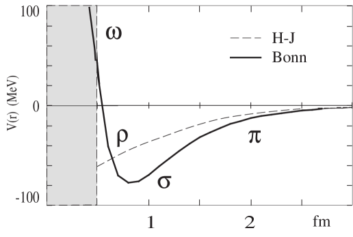
Fig. 1: Average $S$ wave $NN$ potentials.

The short-range repulsive terms have up to now been treated phenomenologically in all potential models. Since the middle 60’s, the hard core is replaced by a soft-core. These forms are demanded to fit the experimental nucleon-nucleon phase shifts. A theoretical derivation of form factor functions for the potential near the origin would require further information on the subnucleonic structure and even explicit modelling of the quark-gluon degrees of freedom, which is beyond our current understanding of quark physics. Quantitatively, the contribution of OPE is about 95% of the total potential contribution for many nuclear properties, as is the case for the deuteron; in a sense the terminology “realistic potential” infers the realistic treatment of OPE and TPE.

More specifically, in the Bonn potentials, all the coupling constants are determined by fitting $np$ scattering data and the deuteron properties. It was claimed recently that the potential models which fit better the $np$ data give poorer agreement for the $pp$ data [10]. From deuteron properties (i.e., the simplest $np$ system), we already know that generally the $np$ components (i.e., mainly T=0 states) of the nucleon-nucleon interaction are more attractive than the $pp$ or $nn$ (i.e., mainly T=0 states) components. Thus fitting only to $np$ scattering data will create a two-nucleon potential which could overestimate the attractive components of the $NN$ force with respect to a unified $np$, $pp$ and $nn$ many-body system. Recently, the Nijmegen group are attempting to provide a potential model by fitting both the $pp$ and $np$ scattering data. The work to derive an effective interaction with this interaction is still in progress.

3 Few-Body and Many-Body Methods

There are many available modern potentials which are based on the analysis of $N\pi$ scattering data within some given energy regimes (for example, up to 350 MeV, the threshold of $\pi$ production ) and the deuteron properties. These potentials are the starting points for a microscopic study of the nuclear dynamics. To this end, the few-body system is an ideal testing-ground of the physics considered. Nowadays the methods used to obtain the nuclear few-body solutions (i.e., in configuration-space or momentum-space) provide very consistent and nearly exact solutions for the bound-state problem. Therefore, the results of the few-body problems will more or less free one from approximations and concentrate on the study of the nucleon dynamics.

Solving the Faddeev-Noyes equations for bound states with a given nucleon-nucleon potential should provide us with the correct binding energy for such systems. Hence to study three-body bound systems, such as ³H and ³He, are particularly important since they are the smallest ones beyond the deuteron for one to quantitatively say something about their properties and the first set of nuclei for one to investigate the importance of hree body interactions. This seemingly simple goal has been pursued by many nuclear physicists for many years, and yet to date, there is still no definitive answer (for a recent review, see [15]). For example, in Table 1 we have presented the benchmark results, which explicitly do not include three-body forces, of the predicted ³H binding energies based upon various modern realistic potentials and as functions of the number of three-body channels. Except for the Bonn potential, the calculated binding energies based on the various $NN$ potential models are about 1 MeV underbound (the experimental binding energy is 8.536 MeV for ³H). The nuclear rms charge radii computed with realistic $NN$ potentials are consistently larger than the experimental values. This discrepancy between experiment and theory is unnerving.

One plausible explanation for the above problem is the presence of a three body force. Table 1 shows that a Hamiltonian of Reid soft-core two-body force plus the Tucson-Melbourne two-pion exchange three-nucleon force (TM3N) [16] can indeed provide additional binding for the trinucleon system. However, these results are highly sensitive to the $\pi$NN form factor and its cutoff mass $\mathchar 3\relax$ [17]. For instance, in a 34-channel calculation, the RSC+TM3N result for cutoff mass $\mathchar 3\relax$=5.8 m_π is 8.86 (MeV), while the binding energies are 7.46 (MeV) and 11.16 (MeV) for $\mathchar 3\relax$=4.1 and 7.1 respectively. Therefore, the current status is that while the correct binding energy can be reproduced with the adjustment of the three-nucleon force, it is done so in a phenomenological manner. On a more fundamental level, three-nucleon interactions have recently been studied by the chiral invariant effective lagrangians [18]. This may be an encouraging direction to fundamentally understand and determine the effective nuclear three-body force.

Table 1: ³H binding energy (in MeV).

potential		RSC	Paris	Nijmegen	Bonn-r
benchmark		7.02	7.31	7.49	8.23
channel		5	9	18	34
RSC		7.02	7.21	7.23	7.35
RSC+TM3N		7.55	8.33	8.93	8.86

It has also been argued that the aforementioned discrepancy between the experimental and calculated binding energy is due to the missing of underlying baryon-meson degree of freedoms. The $\mathchar 1\relax$-isobar and pion degrees of freedom should play some role in the trinucleon binding [19]. After all, the nuclear dynamics is just a low-energy limit of the baryon-meson dynamics. Sauer et al [20] estimates that the presence of a single $\mathchar 1\relax$-isobar provides about 0.3 (MeV) binding and that the three-nucleon force with an intermediate $\mathchar 1\relax$-isobar gives 0.9 (MeV) additional binding, whereas 0.6 (MeV) is lost due to the two-nucleon dispersive effect. Finally, a single $\mathchar 1\relax$ excitation produces about 0.6 (MeV) binding energy, which is not adequate to match the correct binding energy. While such effects can contribute to the binding energies of the respective three body systems, they are not adequate to fully resolve the discrepencies. Another factor which may muddy the water further is relativistic corrections, namely whether or not nuclear spectroscopy is insensitive to the off-shell part of the $NN$ interaction.

The transition from a nuclear few-body system to a nuclear many-body system requires new methodologies to obtain a solution since the traditional few-body techniques no longer apply due to obvious computational difficulties. In particular, the nucleon-nucleon interactions are normally not used directly in the nuclear many-body problem. Instead, effective interactions either “derived” from or motivated by the fundamental interactions are normally used in the many-body context [21]. Hence such interactions must necessarily be intimately linked to the Hilbert space of the calculation. Perhaps the most important ingredient of the many-body systems is to introduce the concept of the mean field. It is often sufficiently accurate to obtain a valid solution of the many-body problem. Based on the mean field assumption, the many body Schrödinger equation for the nucleus can be rewritten as

$$H\psi_{\lambda}(1,2,\cdots,A)=\left(\sum_{i=1}^{A}t_{i}+\frac{1}{2}\sum_{i\neq j=1}^{A}v_{ij}\right)\psi_{\lambda}(1,2,\cdots,A)$$ (1)

$$\hskip 85.35826pt=(H_{0}+H^{\prime})\psi_{\lambda}(1,2,\cdots,A)=E_{\lambda}\psi_{\lambda}(1,2,\cdots,A),$$ (2)

with

$$H_{0}\phi_{\mu}(1,2,\cdots,A)=\sum_{i=1}^{A}\left(t_{i}+u_{i}\right)\phi_{\mu}(1,2,\cdots,A)=E_{\mu}\phi_{\mu}(1,2,\cdots,A)$$ (3)

$$H^{\prime}=\left(\frac{1}{2}\sum_{i\neq j=1}^{A}v_{ij}-\sum_{i=1}^{A}u_{i}\right),$$ (4)

where $t_{i}$ is the kinetic energy, and $u_{i}$ is the mean field that the i-th nucleon feels in the many-body system, i.e., $u_{i}$ represents an average potential contributed by all nucleons in a many-nucleon system. $H^{\prime}$ is the residual interaction.

Basically, there are two ways to deal with the above many-body equations: One is to focus on determining an optimal single-particle mean field $H_{0}$, namely, Hartree-Fock method. The other is to concentrate on figuring out a realistic two-body residual interaction $H^{\prime}$ in order to reproduce the spectroscopy of the many-body system. In the latter case, the technique assumes the solution to be a configuration mixture of Slater determinants. The solution divides neatly into two parts: the calculation of few body terms (one- and two- for most interactions) in a harmonic oscillator basis, followed by the many-body solution in second quantized form of eq.(3). This is the conventional Shell-Model approach. Prior to performing the Shell-Model calculation, one needs to derive the microscopic two-body interactions for a given model space.

Both the Hartree-Fock and the Shell-Model approaches can also be used in conjunction with phenomenological interactions. In the first approach, the use of the Skyrme interaction leads to manageable calculations. It was shown that this interaction is related to the fundamental interaction [22]. On the other hand, for the Shell-Model, an approach based on a fit of the matrix elements in second quantized form [2] attemps to differentiate the quality (or lack thereof) of the fit to experimental data as coming from either the many body aspects of the calculations or from the quality of the two body interaction. These approaches are fundamental in many aspects.

4 Effective Nuclear Interaction for Shell-Model Calculations

In the 60’s, Kuo and Brown presented a classic example to pertubatively derive the microscopic effective interaction (i.e., Shell-Model reaction matrix elements) [23]. Later, a more exact and systematic way to derive the effective two-body interaction for a given model space was developed, namely the Folded-diagram method. This method is reviewed in [24]. There is also a brief review on the $NN$ effective interactions in [25].

For example, using the folded-diagram method, one can determine the 63 two-body matrix elements in the $s$-$d$ shell, which together with the three single-particle energies are the essential input in the $s$-$d$ shell microscopic calculation. Fig.2 gives a comparison of those 63 matrix elements from Hamada-Johnston, Paris and Bonn-A potentials. It shows quite vividly that the different $NN$ potentials can provide very consistent 2-body matrix elements. Only for some matrix elements, especially in the $T=0$ case, are there some discrapencies. However, these small discrapencies can produce substancial differences in the binding enengy calculations as we will see in the next section.

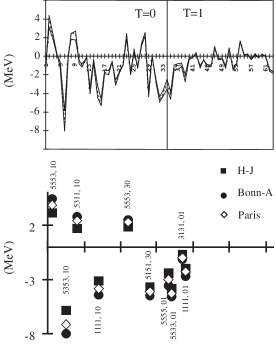
Fig. 2: Comparison of microscopic two-body matrix elements in the $s$-$d$ shell.

5 Conventional Shell-Model Calculations

Nuclei beyond the S-D shell require new techniques to handle the very large model spaces involved. Using massive amount of CPU on the fastest computers [26] while keeping the traditional algorithms is simply not sufficient to model large nuclei. For this reason, there is renewed interest in recent years to develop better, faster and more robust Shell-Model algorithms. It deserves to be mentioned in this direction are the pair Shell-Model algorithm [27] and the Monte-Carlo approaches [28]. The former implements an exact Shell-Model solution for even-even nuclei within a truncated Shell-Model space built from arbitrary pair structures. It generalizes the FDU0 code [29] code which was built from pairs envisioned in the Fermion Dynamical Symmetry Model [30]. These codes can not address directly the question of the worthiness of the fundamental interaction since they seek a solution in a severely truncated model space, which in itself would require an effective interaction with uncertainties. The Monte-Carlo Shell-Model code on the other hand seeks a solution of the many body problem via a Monte-Carlo variational approach. It appears to work will in reproducing the ground state properties of nuclei but suffers, at least up to now, from a lack of convergence for realistic interactions [28].

The Drexel University Shell-Model (DUSM) [31] is another recently completed code to perform Shell-Model calculations which embodies an entirely new algorithm based on permutation group concepts. This is the code we used to perform the calculations to be described in this report despites their simplicity. This code promisses great performance in cases where a full exact Shell-Model solutions are seeked for even-even, even-odd and odd-odd nuclei. It outperforms standard Shell-Model codes [32] by large ( 4 or  5) factors in CPU usage with much reduced disk space and I/O requirements for $J$-$T$ (spin-isospin) coupled spaces.

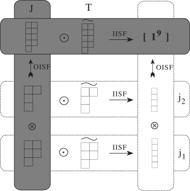
Fig. 3: Two coupling schemes for multishell calculations.

5.1 Drexel University Shell Model Code (DUSM)

The DUSM algorithm starts from the simple observation that Shell-Model calculations are often “multi-shell” in only a single subspace. For instance, a “$J-T$” calculation is multi-shell in the $J$ subspace but single shell in the $T$ subspace ($\tau$=${\textstyle{1\over 2}}$ for all nucleons). Or a Shell-Model calculation for an electronic system is multi-shell in $L$ and single-shell in $S$. The wavefunctions in each subspace have arbitrary permutational symmetry; these symmetry patterns are simply restricted to be conjugate, so as to eventually couple to total antisymmetric wavefunctions. The DUSM coupling scheme is shown in the grayed area of Fig. 3. The DUSM algorithm then proceeds to calculate wavefunctions, coupling coefficents and matrix elements of elementary operators in each shell for each subspace and then in the total space according to the following steps:

1. Compute Coefficients of Fractioal Parentage (CFP) for each shell in each subspace by diagonalysing the Casimir operator of $SU(2j+1)$ in product basis.

2. Compute the matrix elements in all single states of the elementary operators (all combinations of second quantized creation and annihilation operators)

3. Compute the coupling coefficients for the coupling among shells (Outer Product Isoscalar Factors - OISF)

4. Compute the coupling coefficients for the coupling between subspaces (Inner Product Isoscalar Factors - IISF)

5. Compute the matrix elements of the Hamiltonian via a “Sum over Path” in permutation diagrams concepts

6. Diagonalyze the hamiltonian matrix

7. Loop over all total quantum number ($J$ and $T$ for instance) to obtain the global solution

The algorithm presents many advantages over traditional schemes: in particular it avoids computing and storing total space CFPs. This implies much reduced I/O during execution and much less disk storage. Single shell calculations are known to be possible up to very large $J$ and number of particle; DUSM inherits this advantage. The DUSM algorithm uses group theory concepts at all levels to obtain the coupling coefficients, diagonalising the matrix represention of casimir operators of the appropriate groups at all steps, implying very stable numerical schemes. This is an advantage over using Racah formulas to derive the CFP [33] in that no explicit orthogonalization is ever needed. The algorithm can furthermore be implemented (with pointers) without any search since the approach specifies fully the range over all intermediate sums. The approach is fully coupled; it provides full spectra and transitions among the states if required.

This code has recently been completed; we use it in this report to compute some simple cases appropriate to understand the physics of the $NN$ interaction. This does not illustrate by any means the capabilities of DUSM.

5.2 s-d Shell-Model Calculations

We now describe calculations done in various model spaces via DUSM using different effective interactions.

An important factor in the comparison of the experimental binding energies with results from large scale Shell-Model calculations lies in the evaluation of the Coulomb energy; this energy is subtracted from the total experimental binding energy. The relation between total binding energy and the Coulomb term $E_{C}$ is as follow:

$$B_{total}=B_{core}+B_{SM}+E_{C}^{SM},$$ (5)

$$E_{C}^{SM}=E_{C}^{total}-E_{C}^{core},$$ (6)

where $B_{core}$ is the binding energy for the core. $B_{SM}$ is the Shell-Model binding energy related to the core; this term contains the binding energy of the cluster valence-particle plus the binding between the cluster and core. $B_{C}$ is the Coulomb energy.

The total binding energy and core binding energy are listed in the 1993 atomic mass evaluation [34]. Therefore, according to eq. (6), the binding energy calculated from Shell-Model can be directly compared with experimental values $B_{SM}$ when the Coulomb term $E_{c}^{SM}$ is extracted from the experimental values. In ref.[35], the Coulomb energy is estimated with two assumptions: first, for nuclei with a given proton number $Z$, the Coulomb energies are independent of mass,

$$E_{C}(Z,A)=E_{C}(Z,A^{\prime})~{}~{}.$$ (7)

Secondly, for nuclei with same mass $A$, the Shell-Model binding energies measured with respect to the analogue isospin states are the same due to the isospin symmetry for the interactions between identical nucleons (i.e., proton-proton force and neutron-neutron force); consequently, $B_{SM}$ for mirror nuclei are the same, while it differs from odd-odd nuclei due to the excitation energy measured with respect to the ground state,

$$E_{C}^{JT}(Z,A)=E_{C}^{JT}(A-Z,A)~{}~{}.$$ (8)

For instance, when ${}^{16}O$ is considered as an inert core, $B_{SM}(^{18}O)$=$B_{SM}(^{18}Ne)$ (the ground state is (JT)=01), while for ${}^{18}F$, the excitation energy of the (JT)=01 state with respect to its ground state is 1.042 (MeV), thus $B_{SM}(^{18}F)$ + 1.042 = $B_{SM}(^{18}O)$. Notice that this way to estimate the Coulomb energies is not unique. Ref.[35] claimed that the energy difference obtained via different routes is $\leq 150keV$ under the above two assumption.

In more realistic formulation, the Coulomb energy should be closely related to the proton distribution, which in turn should be affected by the neutron distribution. To be more specific, for example, with more neutron outside the core, the attractive interaction between proton and neutron tends to pull the protons towards the surface (i.e., disperse the charge distribution), thus reducing the Coulomb energy. Therefore for nuclei with the same $Z$ but different neutron number $N$, their $E_{C}$ should be different. In fact, such effect is expected to be crucial for neutron rich nuclei.

Alternatively, one can estimate the average Coulomb energy using an empirical formula [36]

$$E_{C}=0.717\frac{Z^{2}}{A^{1/3}}(1-\frac{1.69}{A^{2/3}})~{}~{}(MeV)$$ (9)

The second term in equation above is the Coulomb exchange term which takes into account the effect of dispersion of nucleon due to Pauli exclusive effect. We mention that the theoretical results from the Fermi gas model agree nicely with this empirical formula. Recently, the finite-range droplet model (FRDM) [36] was used to successfully evaluate nuclear ground-state masses and other nuclear structure properties[36], including nuclei between the proton neutron drip lines, showing that the error did not increase with distance from $\beta$ stability. Similar to the Strutinski’s method, FRDM describes nuclear binding energy with two components, one is the so-called macroscopic energy, which is,in some sense, taking care of nuclear bulk behavior, and the second component models the microscopic energy correction accounting for the nuclear shell structures and two-body residual interaction (mainly the pairing effect). The finite range effect of the nuclear force is accounted for by the macroscopic part. Thus the Coulomb energy is further modified [36]. In table 2, we give the empirical Shell-Model binding energies of ¹⁸O, ¹⁸F and ¹⁸Ne using different methods [35, 36]. Note that there are negative values of $E_{C}^{SM}$, which means that $E_{C}(^{18}O)<E_{C}(^{16}O)$ due to charge polarization.

Table 2: The empirical Shell-Model binding energies of ground states.

	(MeV)		${}^{18}O$	${}^{18}F$	${}^{18}Ne$
WB	$B_{SM}$		-12.188	-13.23	-12.188
	$E_{c}^{SM}$		0	3.48	7.666
FRDM	$B_{SM}$		-11.9855	-12.7966	-11.2471
	$E_{c}^{SM}$		-0.2025	3.0466	6.7251

In Table 3, we list the single particle energies for A=18 nuclei. With the s.p. energies and 2-body matrix elements given from sec.4, we now carry out the Shell-Model calculation for the binding energies of ground states. Table 4 presents the calculated binding energies from the microscopic two-body matrix elements of Hamada-Johnston (i.e., Kuo-Brown (KB) interactions which were derived perturbatively in [23]), Bonn-A and Paris potentials. Comparing with Table 2, one can see that KB reproduces correct binding energies, However, Bonn results overbind about 1.8 MeV for $T=1$ and 3.5 MeV for $T=0$. Paris results are between KB and Bonn. Notice that the 2-body matrix elements from Bonn and Paris potentials are derived through a more precise method, namely the folded-diagram approach. These results of Shell-Model calculations are consistent with the few-body calculations with three-body force, where Bonn potential also gives rise to an overbinding.

Table 3: The s.p. energies of A=18 nuclei.

	(MeV)		$d_{\frac{5}{2}}$	$s_{\frac{1}{2}}$	$d_{\frac{3}{2}}$
${}^{18}O$	$E_{C}$=0		-4.144	-3.273	0.941
	$E_{C}$=-0.103		-4.041	-3.170	1.044
${}^{18}F$	$E_{C}$=3.543		-4.144	-3.649	0.856
	$E_{C}$=3.179		-3.780	-3.285	1.220

Fig. 4: Spectra of ¹⁸O.

Fig. 5: Spectra of ¹⁸F.

Table 4: Comparison of binding energies

Nuclei		$E_{B_{exp}}$	KB (MeV)	Bonn (MeV)	Paris (MeV)
${}^{18}O$		kuo	-12.20	-13.96	-13.02
		$E_{C}$=0	-12.19	-13.95	-13.01
		$E_{C}$=-0.103	-11.98	-13.75	-13.02
${}^{18}F$		kuo	-13.36	-16.86	-15.44
		$E_{C}$=3.543	-13.58	-17.09	-15.68
		$E_{C}$=3.179	-12.85	-16.36	-14.95
${}^{18}Ne$			-12.20	-13.96	-13.02
		$E_{C}$=3.543	-12.28	-14.07	-13.12
		$E_{C}$=3.179	-11.55	-13.34	-12.40

The above Shell-Model results for the binding energies are at best confusing: when one starts from a $NN$ soft-core potential, based on effective meson theory with coupling constants being determined by analyzing about a few thousands of $NN$ scattering data values and the deuteron properties, the binding energy results of the microscopic Shell-Model calculations are overbinding. On the other hand, starting from a $NN$ hard-core potential, which is given perturbatively (i.e., the early KB effective interactions), the binding energy is reproduced very well. It is not only that the the binding energy is somewhat better, but the resulting spectra also demonstrate that KB’s presents the best agreement compared with results from other modern potentials. We illustrate this point in Fig.4 and Fig.5 where we show the theoretical and experimental spectra of ¹⁸O and ¹⁸F. It is worth mentioning that KB not only provides the best microscopic shell model results for nuclei in $s$-$d$ shell; recently, systematic Shell-Model calculations for $f$-$p$ nuclei have been carried out by using the Kuo-Brown interaction for the $f$-$p$ shell [26] showing a similar trend.

We may point out that a main difference between the early KB effective interactions and the more recent ones (for example, see [25]) is about the treatment of the folded diagrams. For the former the folded diagrams were ignored, with the effective interaction given merely by the bare-G and the second-order core polarization diagrams. These diagrams are usually referred to as $G$ and $G_{3p1h}$ in the literature [37]. For the later, certain types of folded diagrams are included to all orders using a $\hat{Q}$-box formulation [37]. What we have found in this work may indicate the need of a further investigation of the folded diagrams. There may be some other physical processes, which may counterbalance the effect of the folded diagrams and which have not been investigated. When this is done, it may be possible that the effective interaction will again be mainly given by $G$ and $G_{3p1h}$ alone, making life simpler.

6 Comments

In summary, we have given a brief review of the microscopic Shell-Model studies, and mentioned the recently developed Drexel University Shell Model (DUSM) code, which implements a new Shell-Model algorithm. We presented simple Shell-Model calculations to illustrate the progress made in this field and discussed some significant problems which remain in connection to the effective interactions used.

References

- [1] For instance, the description of shell nuclei in: J.P. Elliott, Proc. Roy. Soc. (London) A245 (1958)128,562,182,379.
- [2] A good example is the emperical Shell-Model study with Wildenthal Interaction for shell, see: B.A. Brown, W.A. Richter, R.E. Julies and B.H. Wildenthal, Ann. Phys. 182 (1988)191.
- [3] B.A. Brown and B.H. Wildenthal, Ann. Rev. Nucl. Part. Sci. 38 (1988) 29.
- [4] K. Allaart, E. Boeker, G. Bonsignori, M. Sovoia and Y.K. Gambhir, Physics Report 169 (1988) 209, J.Q. Chen, X.W. Pan and B.Q. Chen, An exact shell model calculation in the S-D subspace (preprint 1993).
- [5] N.I. Karchev and A.A. Slavnov, Theor. Math. Phys. 65 (1985) 192.
- [6] F.Q. Liu and X.W. Pan, From QCD to a QCD string Hadron Dynamics (to be submitted).
- [7] H. Yukawa, Proc. Math. Soc. Japan 17 (1935) 48.
- [8] W.N. Cottingham, M. Lacombe, B. Loiseau, J.M. Richard and R. Vinh Mau, Phys. Rev. D8 (1973) 8; M. Lacombe, B. Loiseau, J.M. Richard and R. Vinh Mau, J.Cote, P. Pires and R. de Tourreil, Phys. Rev. C21 (1980) 861.
- [9] R. Machleidt, K. Holinde and Ch. Elster, Phys. Rep. 149 (1987) 1; R. Machleidt, Adv. Nucl. Phys. 19 (1989) 189.
- [10] V. Stoks and J.J. de Swart, Phys. Rev. C47 (1993) 761.
- [11] T. Hamada and I.D. Johnston, Nucl. Phys. 34 (1962) 382.
- [12] R.V. Reid,Jr., Ann. Phys. (N.Y.) 50 (1968) 411.
- [13] R.B. Wiringga, R.A. Smith and T.L. Ainsworth, Phys. Rev. C29 (1984) 1207.
- [14] S. Weinberg, Nucl. Phys. B363 (1991) 3; Phys. Lett. B251 (1990) 288; Phys. Lett. B295 (1992) 114.
- [15] B.F. Gibson, Nucl. Phys.A543, 1C (1992); and the reference therein.
- [16] S.A. Coon, M.D. Scadron,P.C. McNamee , B.R. Barret, D.W. E. Blatt, B.H.J. McKellar, Nucl. Phys. A317 (1979) 242.
- [17] S. Ishikawa, T. Sasakawa, T. Sawata and T. Ueda, Phys. Rev. Lett. 53, 1877 (1984).
- [18] S. Weinberg, Phys. lett. B295 (1992)114; U.van Kolck, few-nucleon forces from Chiral Lagrangians, (DOE/ER/40427-30-N93).
- [19] A recent review on this issue is in: P. U. Sauer, Nucl. Phys. A543 (1992) 291c.
- [20] C. Hajduk, P.U. Sauer and W. Strueve, Nucl. Phys. A405 (1983) 581.
- [21] For example, see: M.K. Kirson, Nuclear Shell Models, ed. by M. Vallières and B.H. Wildenthal, (World Scientific 1985).
- [22] J.W. Negele, Phys. Rev. C1 (1970) 1260.
- [23] T.T.S Kuo and G.E. Brown, Nucl. Phys. 85 (1966)40.
- [24] A review paper is given in: T.T.S. Kuo and E. Osnes, Lecture Notes in Physics Vol.364 (Springer-Verlag 1990).
- [25] T.T.S. Kuo, Nucl. Phys. A570 (1994) 173c.
- [26] H. Nakada, T. Sebe and T. Otsuka, Nucl. Phys. A571 (1994) 467.
- [27] J.Q. Chen, B.Q. Chen and A. Klein, Nucl. Phys. A554 (1993) 61; J.Q. Chen, X.W. Pan and B.Q. Chen, Nuclear-Pair Shell Model: even system, (preprint 1994).
- [28] C.W. Johnson, S.E. Koonin, G.H. Lang and W.E. Ormand, Phys. Rev. Lett. 69 (1992) 3157.
-
[29]
M. Vallières and H. Wu, in
Computational Nuclear Physics 1,
ed. by K. Langanke, et al (Springer–Verlag 1991) p. 1. - [30] C.L. Wu, D.H. Feng and M. Guidry, in Advances in Nuclear Physics, edited by J.W. Negele and E. Vogt (Plenum, New York, 1994), Vol.21, p.1.
- [31] M. Vallières and A. Novoselsky, Drexel University Shell Model (DUSM code), (1994).
- [32] B.A. Brown, A. Etchegoyen and W.D.M. Rae, The computer code OXBASH, MSU-NSCL number 524 (nucl-th/9406020 for retrieving the code).
- [33] X. Ji and M. Vallières, Phys. Rev. C35 (1987) 1583.
- [34] G. Audi and A.H. Wapstra, Nucl. Phys. A565 (1993) 1.
- [35] E.K. Warburton and B.A. Brown, Phys. Rev. C46 (1992) 923.
- [36] W.D. Myers and W.J. Swialecki, Nucl. Phys. A81 (1966)1,4,39,83; P. Moller, J.R. Nix, W.D. Myers and W.J. Swialecki, Nuclear Ground-State Masses and Deformations (preprint 1993).
- [37] J. Shurpin, D. Strottman and T.T.S. Kuo, Nucl. Phys. A408 (1983) 310.