SNUTP 95-043

Chiral Lagrangian Approach to Exchange Vector Currents in Nuclei
Tae-Sun Park^(a), Dong-Pil Min^(a) and Mannque Rho^(b)
Institute for Nuclear Theory, University of Washington
Seattle, WA 98195, U.S.A.
ABSTRACT

Exchange vector currents are calculated up to one-loop order (corresponding to next-to-next-to-leading order) in chiral perturbation theory. As an illustration of the power of the approach, we apply the formalism to the classic nuclear process $n+p\rightarrow d+\gamma$ at thermal energy. The exchange current correction comes out to be $(4.5\pm 0.3)$ % in amplitude giving a predicted cross section $\sigma=(334\pm 3)\ {\mbox{m}b}$ in excellent agreement with the experimental value $(334.2\pm 0.5)\ {\mbox{m}b}$. Together with the axial charge transitions computed previously, this result provides a strong support for the power of chiral Lagrangians in nuclear physics. As a by-product of our results, we suggest an open problem in the application of chiral Lagrangian approach to nuclear processes that has to do with giving a physical meaning to the short-range correlations that play an important role in nuclei.

$(a)$ Permanent address : Department of Physics and Center for Theoretical Physics, Seoul National University, Seoul 151-742, Korea

$(b)$ Permanent address : Service de Physique Théorique, CEA Saclay, 91191 Gif-sur-Yvette, France

1 Introduction

Nuclear responses to electroweak probes are described by matrix elements of the corresponding currents. The major contribution comes from one-body currents, specifically, the sum of the currents of each nucleon. The principal corrections come from exchange currents (or meson-exchange currents) that consist of two-body and higher-body currents. By now there exist a large number of unambiguous experimental evidence [1] for the presence and structure of meson-exchange currents. While phenomenological in character, the approaches taken so far can describe the large bulk of experiments [2] rather successfully, providing us our progressive understanding of nuclear processes. To the extent that nucleon-nucleon interactions are now fairly accurately understood, one can have a great deal of confidence in the theoretical tool with which the effect of exchange currents is calculated. There remains however the fundamental question as to how our phenomenological understanding of nuclear forces and associated meson currents can be linked to the fundamental theory of strong interactions, QCD.

In the modern understanding of QCD, it is the spontaneous breaking of chiral symmetry associated with the light quarks that predominantly governs the structure of low-energy hadrons as well as the forces mediating between them. In fact, the full content of the gauge theory of strong interactions, QCD, can be expressed at low energy by a systematic chiral expansion starting with effective chiral Lagrangians [3]. Stated more strongly, such an approach, known as chiral perturbation theory (ChPT), while reproducing the current algebra, is now considered to be exactly equivalent to QCD in long wavelength regime [4]. The question that is immediately posed here is whether or not one can describe nuclear processes from the chiral perturbation theory point of view.

Two recent developments suggest that the answer to this question is affirmative. The first is the work of Weinberg [5] and Ordóñez, Ray and van Kolck [6] on understanding nuclear forces from chiral Lagrangians. The second is the explanation by the present authors [7] of the enhanced axial-charge transitions in heavy nuclei in terms of exchange axial currents in chiral perturbation theory treated to the same chiral order as for nuclear forces. Both of these two works provide a systematic and consistent field-theory-based understanding of the nuclear processes and validate at the same time the traditional approaches to the processes. In this paper, we present one more case where the chiral Lagrangian scores a stunning success, namely, the radiative neutron capture

$$n+p\rightarrow d+\gamma$$ (1)

at threshold. This result was briefly reported in a Letter [8]. Here we shall go into greater details of the calculation involved for the process (1).

Historically, the process (1) was first explained quantitatively two decades ago by Riska and Brown [9] who showed that the $\sim 10\%$ discrepancy between the experimental cross-section and the theoretical impulse approximation prediction is eliminated by exchange currents. Riska and Brown computed, using realistic hard-core wavefunctions, the two one-pion-exchange diagrams initially suggested in 1947 by Villars [10] plus the $\omega$ and $\Delta$ resonance diagrams. That the dominant contributions to electroweak exchange currents could be gotten from current-algebra low-energy theorems was suggested by Chemtob and Rho [11] who gave a systematic rule for organizing the leading exchange-current diagrams effective at low energy and momentum. Although suspected since the Yukawa force was introduced, the work of Riska and Brown was the first unequivocal evidence for the role of mesons, in particular that of pions, in nuclear interactions. In this paper, we show that the terms considered by Riska and Brown are a main part of the terms that figure in chiral perturbation theory to next-to-next-to-leading (N²L) order and that when completed by the rest of the N²L order terms, chiral perturbation theory works impressively, confirming on the one hand the work of Riska and Brown [9] and on the other hand the earlier (“chiral filter”) conjecture of Kubodera, Delorme and Rho [12].

In all cases studied so far, one is limited to long wavelength processes, with the typical energy/momentum scale $Q$ much less than the chiral symmetry scale $\Lambda_{\chi}\sim 4\pi f_{\pi}\sim 1$ GeV. This is because ChPT is an expansion in $Q/\Lambda_{\chi}$ and its practical value lies where $Q/\Lambda_{\chi}\ll 1$. For nuclear physics, where both baryons and mesons enter on the same footing, the heavy-fermion formalism as discussed in [5, 13] proves to be convenient for making a systematic expansion in derivative on pion fields as well as on baryons fields, $\partial/\Lambda_{\chi}$ and in $m_{\pi}/\Lambda_{\chi}$ where $m_{\pi}$ is the pseudo-Goldstone boson mass. In this formalism, the nucleon mass is regarded as heavy, $m_{{}_{\rm N}}\simeq\Lambda_{\chi}$.

As in [5], the expansion is organized by the power $\nu$ in $Q^{\nu}$. This expansion will be reviewed in the next section. Here we remark briefly how kinematical considerations affect the chiral counting rule, modifying it from the naive counting rule. The modification comes from the fact that the space part of the vector current and the time part of the axial-vector current $(V^{i},\,A^{0})$ are proportional to $(\gamma^{i},\,\gamma_{5}\gamma^{0})$ and hence are suppressed compared to the other part of the currents, $(V^{0},\,A^{i})$. The correct counting for one-body currents in two-body systems is $(V^{i},\,A^{0})_{\rm 1B}={\cal O}(Q^{-2})$. Compared to these one-body currents, the leading two-body current contributions are of order ${\cal O}(Q)$ and the one-loop corrections are of order ${\cal O}(Q^{3})$. Thus from the point of view of the chiral expansion, the two-body currents at one-loop order correspond to next-to-next-to-leading (N²L) order. This is the order that was computed in the case of the nuclear axial-charge transitions studied in [7] and that will be adopted for the vector current matrix element for the process (1). Three-body (and higher-body) currents are suppressed for exactly the same reason as for the suppression of 3-body forces discussed by Weinberg [5]: the resulting 3-body currents are of order ${\cal O}(Q^{4})$ compared to the 1-body currents.

Given these counting rules, the ChPT in nuclear systems can be made to correspond to computing Feynman diagrams involving external fields in the increasing power $\nu$ embedded inside the most general process describing the transition from the initial nuclear state to the final nuclear state with interactions taking place before and after the current insertion. This strategy is essentially the same as what was first suggested, with somewhat ad hoc assumptions, in [11]. What this means in practice is that we are to take the most realistic nuclear wave functions and calculate the transition matrix elements with the ChPT graphs computed to the maximum possible order of chiral expansion. This allows us to fix the “counter terms” in the chiral expansion from experiments. At the present stage of our understanding on the role of chiral symmetry in nuclear systems, this seems to be the only practical attitude to take in confronting nuclear dynamics. We might point out that this point of view is consistent with the approach advocated by Weinberg [5] in his treatment of nuclear forces, in particular many-body forces. An important consequence of this strategy is then that only the current operators obtainable by ChPT are to be kept. This implies mainly two things. Firstly, it implies that short-wavelength effects are to be “filtered out”. Secondly, it implies that $n$-body currents with $n>2$ are suppressed in nuclear systems with the mass number $A>2$ in the same sense that $n$-body forces are suppressed [5]. Of particular importance of the first implication is that when the currents are put in coordinate space, shorter-range interactions for $r_{12}\mathrel{\raise 1.29167pt\hbox{$<$\kern-7.5pt\lower 4.30554pt\hbox{$\sim$}}}r_{c}$ – where $r_{c}$ is the hard core radius – cannot contribute in ChPT. This is because the “short-range correlations” that play an important role in nuclear observables represent those degrees of freedom that cannot be accessed by chiral perturbation expansion. Clearly this strategy would make sense only if the result does not sensitively depend on the precise value of the “hard-core” size $r_{c}$, within the relevant range for application in nuclei to the order considered, say, $\Lambda_{\chi}^{-1}\mathrel{\raise 1.29167pt\hbox{$<$\kern-7.5pt\lower 4.30554pt\hbox{$\sim$}}}r_{c}\mathrel{\raise 1.29167pt\hbox{$<$\kern-7.5pt\lower 4.30554pt\hbox{$\sim$}}}(2m_{\pi})^{-1}$. Note that this is roughly the range that can be reasonably described in ChPT for the NN potential [6].

This paper is organized as follows. In section 2, chiral perturbation theory as appropriate for the problem at hand will be briefly summarized. The main purpose of this section is to define the notations and indicate the strategy specific to nuclear problems as outlined above and detailed in [7]. For a general and comprehensive review of chiral perturbation theory, we refer to recent review articles [16]. Section 3 deals with the derivation of the exchange electromagnetic currents in nuclei to N²L order for vanishingly small momentum transfers. The formulas derived in Section 3 are applied in Section 4 to the classic nuclear process (1). Some further remarks and conclusion are given in Section 5. The Appendices give detailed formulas used in the main text.

2 Chiral Perturbation Theory

Here we shall briefly review the specific aspect of chiral perturbation theory (ChPT) adopted for our calculation to one-loop order. This section is organized as follows. We start, in Section 2.1, with a rederivation of Weinberg’s counting rules with a slight generalization. The relevant chiral Lagrangians in heavy-fermion formalism (HFF) will be written down in Section 2.2 and the renormalization procedure within HFF in Section 2.3. The particular feature of ChPT in nuclear physics will be described in Section 2.4.

2.1 Counting rules

Here we rederive and generalize somewhat Weinberg’s counting rule [5] along the line described in [7]. Although we shall not consider explicitly the vector-meson degrees of freedom, we include them here in addition to pions and nucleons. Much of what we will obtain later without vector mesons turn out to be valid in their presence. In our work, we consider the vector-meson masses – which are comparable to the chiral scale $\Lambda_{\chi}$ – as heavy compared to the momentum probed $Q$ – say, scale of external three momenta or $m_{\pi}$. In dense medium, the situation is different as discussed in [15]. There the vector-meson masses can be considered small, in the sense of Georgi’s vector limit. In our discussions, we do not encounter the dense regime in which vector-meson masses drop as a function of density.

In establishing the counting rule, we make the following assumptions: Every intermediate meson (whether heavy or light) carries a four-momentum of order of $Q$. In addition we assume that for any loop, the effective cut-off in the loop integration is of order of $Q$. We will specify what this means physically when we discuss specific processes, for this clarifies the limitation of the chiral expansion scheme.

An arbitrary Feynman graph can be characterized by the number $E_{N}(E_{H},E_{E})$ of external – both incoming and outgoing – nucleon (vector-meson, external field) lines, the number $L$ of loops, the number $I_{N}(I_{\pi},\ I_{H})$ of internal nucleon (pion, vector-meson) lines and the number of $C$ disconnected pieces of the Feynman graphs. For an connected graph, for example, we should have $C=1$. Each vertex can in turn be characterized by the number $d_{i}$ of derivatives and/or of $m_{\pi}$ factors and the number $n_{i}$ $(h_{i},e_{i})$ of nucleon (vector-meson, external field) lines attached to the vertex. Now for a nucleon intermediate state of momentum $p^{\mu}=m_{{}_{\rm N}}v^{\mu}+k^{\mu}$ where $k^{\mu}={\cal O}(Q)$ and $v^{\mu}$ is a constant 4-vector with $v^{\mu}\simeq(1,\,{\mbox{\boldmath$0$\/}})$, we acquire a factor $Q^{-1}$ since

$$S_{F}(m_{{}_{\rm N}}v+k)=\frac{1}{v\cdot k}={\cal O}(Q^{-1}),$$ (2)

where we have used the propagator obtained by the HFF which will be explained in the next section. An internal pion line contributes a factor $Q^{-2}$ since

$$\Delta_{F}(q^{2};m_{\pi}^{2})=\frac{1}{q^{2}-m_{\pi}^{2}}={\cal O}(Q^{-2})$$

while a vector-meson intermediate state contributes $Q^{0}$ $(\sim O(1))$ as one can see from its propagator, noting that $D_{F}^{\mu\nu}(q^{2};m_{V}^{2})=\left(-g^{\mu\nu}+\frac{q^{\mu}q^{\nu}}{m_{V}^{2}}\right)\Delta_{F}(q^{2};m_{V}^{2})={\cal O}(Q^{0})\,\Delta_{F}(q^{2};m_{V}^{2})$,

$$\Delta_{F}(q^{2};m_{V}^{2})=\frac{1}{q^{2}-m_{V}^{2}}\simeq\frac{1}{-m_{V}^{2}}={\cal O}(Q^{0})$$ (3)

where $m_{V}$ represents a generic mass of vector mesons. And a loop contributes a factor $Q^{4}$ because its effective cut-off is assumed to be of order of $Q$. Finally, the $C$ separated pieces of the Feynman graph contributes a factor $Q^{4(1-C)}$ due to the $(C-1)$ times of the energy-momentum conservation factor, $(2\pi)^{4}\delta^{4}(\sum_{i}p_{i})$ where $(\sum_{i}p_{i})$ denote the sum of incoming and outgoing momenta of a separate piece of the Feynman graph.

We thus arrive at the counting rule that an arbitrary graph is characterized by the factor $Q^{\nu}$ with

$$\nu=-I_{N}-2I_{\pi}+4L+4-4C+\sum_{i}d_{i}$$ (4)

where the sum over $i$ runs over all vertices of the graph. Using the identities, $I_{\pi}+I_{H}+I_{N}=L+V-C$ where $V$ denotes the total number of vertices of the Feynman graph, $I_{H}=\frac{1}{2}(\sum_{i}h_{i}-E_{H})$, $I_{N}=\frac{1}{2}(\sum_{i}n_{i}-E_{N})$ and $\sum_{i}e_{i}=E_{E}$, we can rewrite the counting rule

$$\nu=4-2C-\left(\frac{E_{N}}{2}+E_{H}+E_{E}\right)+2L+\sum_{i}{\bar{\nu}}_{i},\ \ \ \ \ {\bar{\nu}}_{i}\equiv d_{i}+\frac{n_{i}}{2}+h_{i}+e_{i}-2.$$ (5)

We recover the counting rule derived by Weinberg [5] if we set $E_{H}=h_{i}=0$ and $E_{E}=e_{i}=0$. With non-zero external heavy meson lines, it is generally hard to satisfy our condition that all the internal lines should carry momenta of order of $Q$. But there is no limitation on the number of $h_{i},\,e_{i}$ and $E_{E}$.

The quantity ${\bar{\nu}}_{i}$ is defined so that

$${\bar{\nu}}_{i}=\left(d_{i}+\frac{n_{i}}{2}+h_{i}+e_{i}-2\right)\geq 0.$$ (6)

This is guaranteed by chiral symmetry [5] even in the presence of external fields. In the absence of external fields (as in nuclear forces),

$$d_{i}+\frac{n_{i}}{2}+h_{i}-2\geq 0.$$ (7)

This means that the leading order effect comes from graphs with vertices satisfying

$$d_{i}+\frac{n_{i}}{2}+h_{i}-2=0\,.$$ (8)

Examples of vertices of this kind are: $\pi^{k}NN$ with $k\geq 1\,(d_{i}=1,\ n_{i}=2,\ h_{i}=0)$, $hNN\,(d_{i}=0,\ n_{i}=2,\ h_{i}=1)$, four-Fermi contact interactions, $(d_{i}=0,\ n_{i}=4,\ h_{i}=0)$, $h\pi^{k}$ with $k\geq 1\,(d_{i}=1,\ n_{i}=0,\ h_{i}=1)$, etc where $h$ denotes vector-meson fields. In $NN$ scattering or in nuclear forces, $\frac{E_{N}}{2}=2$ and $E_{H}=0$, and so we have $\nu\geq 0$. The leading order contribution corresponds to $\nu=0$, coming from three classes of diagrams; one-pion-exchange, one-vector-meson-exchange and four-Fermi contact graphs. In $\pi N$ scattering, $\frac{E_{N}}{2}=1$ and $E_{H}=0$, we have $\nu\geq 1$ and the leading order comes from nucleon Born graphs, seagull graphs and one-vector-meson-exchange graphs.

In the presence of external fields denoted generically ${\cal E}$, the condition becomes [17]

$$\left(d_{i}+\frac{n_{i}}{2}+h_{i}-2\right)\geq-1\,.$$ (9)

The difference from the previous case comes from the fact that a derivative is replaced by a gauge field. The equality holds only for the vertices ${\cal E}\pi^{j}NN$ with $j\geq 0$ ($d_{i}=h_{i}=0,\,n_{i}=2$), ${\cal E}h\pi^{j}$ with $j\geq 0$ ($h_{i}=1,\,n_{i}=d_{i}=0$) and ${\cal E}\pi^{k}$ with $k\geq 1$ ($h_{i}=n_{i}=0$, $d_{i}=1$). We will later show that this is related to the “chiral filter” phenomenon. The condition (9) plays an important role in determining exchange currents. Apart from the usual nucleon Born terms which are in the class of “reducible” graphs and hence do not enter into our consideration, we have two graphs that contribute in the leading order to the exchange current: the “seagull” graphs and “pion-pole” graphs , both of which involve a vertex with ${\bar{\nu}}_{i}=0$. On the other hand, a vector-meson-exchange graph involves a ${\bar{\nu}}_{i}=2$ vertex. This is because $d_{i}=1,\ h_{i}=2$ at the ${\cal E}hh$ vertex and $d_{i}=1$, $n_{i}=2$, $h_{i}=1$ at the ${\cal E}hNN$ vertex, where ${\cal E}$ denotes external fields. Therefore vector-exchange graphs are suppressed by power of $Q^{2}$. This counting rule is the basis for establishing the chiral filtering even when vector mesons are present (see Appendix C). Thus the results we obtain without explicit vector mesons are valid more generally.

We now focus on the nuclear responses to electroweak probes. Denoting the vector ($V^{\mu}$) and axial-vector currents ($A^{\mu}$) collectively by $G^{\mu}$, we decompose the latter in terms of the number of nucleons involved:

$$G^{\mu}=G^{\mu}_{\rm 1B}+G^{\mu}_{\rm 2B}+\cdots.$$ (10)

In principle, there will be $n$-body currents for $N\geq n\geq 1$ in $N$-body systems. Compared to the leading 2-body currents, the leading $3$-body currents are suppressed by a factor ${\cal O}(Q^{2}/\Lambda_{\chi}^{2})$ from the counting rule eq.(5) and further suppressed by a factor ${\cal O}(Q/\Lambda_{\chi})$ for exactly the same reason as for the suppression of the 3-body forces [5]. Thus the net suppression factor is of order $(Q/\Lambda_{\chi})^{3}$ compared to the 2-body currents. We can therefore safely ignore three-body and higher-body currents. Limiting ourselves to the two-body subsystem, we have $E_{H}=0$, $\frac{E_{N}}{2}=2$ and $E_{E}=1$. The counting rule reads

$$\nu=1-2C+2L+\sum_{i}{\bar{\nu}}_{i},\ \ \ \ \ {\bar{\nu}}_{i}\equiv d_{i}+\frac{n_{i}}{2}+h_{i}+e_{i}-2$$ (11)

where $C=2$ for one-body currents and $C=1$ for two-body currents. This counting rule would naively imply $G^{\mu}_{\rm 1B}={\cal O}(Q^{-3})$ and $G^{\mu}_{\rm 2B}={\cal O}(Q^{-1})$. But as mentioned in Introduction, there is a further suppression factor of order $Q/\Lambda_{\chi}$ for $(V^{i},\,A^{0})_{\rm 1B}$ and $(V^{0},\,A^{i})_{\rm 2B}$, with $i=1,\,2,\,3$. The suppression of one-body currents can be understood simply by recalling that the leading-order vector and axial-vector one-body currents are proportional, respectively, to ${\bar{u}}\gamma^{\mu}u=({\cal O}(1),{\cal O}(Q/m_{{}_{\rm N}}))$ and ${\bar{u}}g_{A}\gamma^{\mu}\gamma_{5}u=({\cal O}(Q/m_{{}_{\rm N}}),{\cal O}(1))$ where $u$ denotes the spinor of the nucleon. As for the two-body currents, the same suppression factor appears with the interchange of the role of the vector and axial-vector currents. The effective chiral counting for the currents is summarized in Table 1.

	$V^{i}$ and $A^{0}$	$V^{0}$ and $A^{i}$	$G^{\mu}$ (naive)
1-body	${\cal O}(Q^{-2})$	${\cal O}(Q^{-3})$	${\cal O}(Q^{-3})$
2-body (leading)	${\cal O}(Q^{-1})$	${\cal O}(Q^{0})$	${\cal O}(Q^{-1})$
2-body (1-loop correction)	${\cal O}(Q^{1})$	${\cal O}(Q^{1})$	${\cal O}(Q^{1})$
$\langle M_{\rm 2B}\rangle/\langle M_{\rm 1B}\rangle$	${\cal O}(Q^{1})$	${\cal O}(Q^{3})$	${\cal O}(Q^{2})$

Table 1: The chiral counting for the vector and axial-vector currents for two-body subsystems. The last row gives the ratio of the amplitude of the two-body currents compared to that of the one-body currents. The last column shows the naive counting.

One can see immediately that the effect of the two-body currents can be sizable while the loop corrections are small for the space component of the vector current and the time component of the axial-vector current. This feature was noted sometime ago [12].

2.2 Effective chiral Lagrangian in heavy-baryon formalism

The effective chiral Lagrangian that consists of pions and nucleons involving lowest derivative terms takes the form [18],

$${\cal L} = {\overline{N}}\left[i\gamma^{\mu}D_{\mu}-m_{{}_{\rm N}}+ig_{A}\gamma^{\mu}\gamma_{5}\Delta_{\mu}\right]N-\frac{1}{2}\sum_{A}C_{A}\left({\overline{N}}\Gamma_{A}N\right)^{2}$$ (12)

$$+\,\frac{f_{\pi}^{2}}{4}{\rm Tr}\left(\nabla_{\mu}\Sigma^{\dagger}\nabla^{\mu}\Sigma\right)+\frac{f_{\pi}^{2}}{4}m_{\pi}^{2}{\rm Tr}(\Sigma+\Sigma^{\dagger})+\cdots,$$

where

$$\Delta_{\mu} = \frac{1}{2}\left\{\xi^{\dagger},{\partial_{\mu}}\xi\right\}-\frac{i}{2}\xi^{\dagger}({\cal V}_{\mu}+{\cal A}_{\mu})\xi+\frac{i}{2}\xi({\cal V}_{\mu}-{\cal A}_{\mu})\xi^{\dagger},$$

$$\nabla_{\mu}\Sigma = {\partial_{\mu}}\Sigma-i({\cal V}_{\mu}+{\cal A}_{\mu})\Sigma+i\Sigma({\cal V}_{\mu}-{\cal A}_{\mu})$$ (13)

with the external gauge fields ${\cal V}_{\mu}={\vec{\cal V}}_{\mu}\cdot\frac{{\vec{\tau}}}{2}$ and ${\cal A}_{\mu}={\vec{\cal A}}_{\mu}\cdot\frac{{\vec{\tau}}}{2}$. Here $m_{{}_{\rm N}}\simeq 939$ MeV is the nucleon mass, $g_{A}\simeq 1.25$ is the axial coupling constant, $f_{\pi}\simeq 93$ MeV is the pion decay constant and $m_{\pi}\simeq 139$ MeV is the pion mass. The ellipsis stands for higher derivative and/or symmetry-breaking terms that will be specified later as needed. Under chiral SU(2)$\times$SU(2) transformation, the chiral field $\Sigma={\rm exp}(i\frac{{\vec{\tau}}\cdot{\vec{\pi}}}{f_{\pi}})$ transforms as $\Sigma\rightarrow g_{\mbox{\tiny R}}\Sigma g_{\mbox{\tiny L}}^{\dagger}$ ($g_{\mbox{\tiny R}},g_{\mbox{\tiny L}}\in$ SU(2)) and the covariant derivative transforms the same as $\Sigma$ does,

$$\nabla_{\mu}\Sigma = {\partial_{\mu}}\Sigma-i({\cal V}_{\mu}+{\cal A}_{\mu})\Sigma+i\Sigma({\cal V}_{\mu}-{\cal A}_{\mu})$$ (14)

$$\rightarrow g_{\mbox{\tiny R}}\,\nabla_{\mu}\Sigma\,g_{\mbox{\tiny L}}^{\dagger}$$

with the external gauge fields transforming locally

$${\cal V}_{\mu}+{\cal A}_{\mu} \rightarrow {\cal V}_{\mu}^{\prime}+{\cal A}_{\mu}^{\prime}=g_{\mbox{\tiny R}}({\cal V}_{\mu}+{\cal A}_{\mu})g_{\mbox{\tiny R}}^{\dagger}-i{\partial_{\mu}}g_{\mbox{\tiny R}}\cdot g_{\mbox{\tiny R}}^{\dagger},$$

$${\cal V}_{\mu}-{\cal A}_{\mu} \rightarrow {\cal V}_{\mu}^{\prime}-{\cal A}_{\mu}^{\prime}=g_{\mbox{\tiny L}}({\cal V}_{\mu}-{\cal A}_{\mu})g_{\mbox{\tiny L}}^{\dagger}-i{\partial_{\mu}}g_{\mbox{\tiny L}}\cdot g_{\mbox{\tiny L}}^{\dagger}.$$

The non-linear realization of chiral symmetry is expressed in terms of $\xi=\sqrt{\Sigma}={\rm exp}(i\frac{{\vec{\tau}}\cdot{\vec{\pi}}}{2f_{\pi}})$ and $h=h(\xi,g_{\mbox{\tiny L}},g_{\mbox{\tiny R}})$ defined with $\xi$

$$\xi\rightarrow g_{\mbox{\tiny R}}\xi h^{\dagger}=h\xi g_{\mbox{\tiny L}}^{\dagger}.$$

The nucleon field $N$ transforms as a matter field, i.e, $N\rightarrow hN$, and its covariant derivative as $D_{\mu}N\rightarrow hD_{\mu}N$ while $\Delta_{\mu}\rightarrow h\Delta_{\mu}h^{\dagger}$ where

$$D_{\mu}N = ({\partial_{\mu}}+\Gamma_{\mu})N,$$

$$\Gamma_{\mu} = \frac{1}{2}\left[\xi^{\dagger},\,{\partial_{\mu}}\xi\right]-\frac{i}{2}\xi^{\dagger}({\cal V}_{\mu}+{\cal A}_{\mu})\xi-\frac{i}{2}\xi({\cal V}_{\mu}-{\cal A}_{\mu})\xi^{\dagger}.$$ (15)

Note that $h(\xi,g_{\mbox{\tiny L}},g_{\mbox{\tiny R}})$ is a complicated local function of $\xi$, $g_{\mbox{\tiny L}}$ and $g_{\mbox{\tiny R}}$, the explicit form of which is not needed.

We have included the four-Fermi non-derivative contact term studied by Weinberg [5]. We shall ignore possible four-Fermi contact terms involving quark mass terms and derivatives except for counter terms needed later. They are not relevant to the chiral order (in the sense defined precisely later) that we are working with. The explicit chiral symmetry breaking is included minimally in the form of the pion mass term. Higher order symmetry breaking terms do not play a role in our calculation.

For completeness – and to define our notations – we sketch here the basic element of the heavy-fermion formalism (HFF) [19] applied to nuclear systems as developed by Jenkins and Manohar [20] wherein the nucleon is treated as a heavy fermion. As stressed in Introduction, the relativistic formulation of ChPT works well when only mesons are involved but it does not work when baryons are involved since while space derivatives on baryons fields can be arranged to appear on the same footing as four-derivatives on pion fields, the time derivative on baryon fields picks up a term of order of the chiral symmetry breaking scale and hence cannot be used in the chiral counting. This problem is avoided in the HFF. To set up the HFF, the fermion momentum is written as

$$p^{\mu}=m_{{}_{\rm N}}v^{\mu}+k^{\mu}$$ (16)

where $v^{\mu}$ is the $4$-velocity with $v^{2}=1$, and $k^{\mu}$ is the small residual momentum. (In the practical calculation that follows, we will choose the heavy-fermion rest frame $v^{\mu}=(1,{\mbox{\boldmath$0$\/}})$.) From the conventional nucleon field $N(x)$, we define heavy fermion field $B_{v}(x)$ for a given four-velocity $v^{\mu}$, by

$$B_{v}(x)={\mbox{e}}^{im_{{}_{\rm N}}\,v\cdot x}N(x),$$ (17)

which we divide into two parts,

$$B_{v}=B_{v}^{(+)}+B_{v}^{(-)}\equiv\frac{1+{\not{\!v}}}{2}B_{v}+\frac{1-{\not{\!v}}}{2}B_{v}.$$ (18)

As defined, $B_{v}^{(+)}(B_{v}^{(-)})$ can be identified as positive (negative) energy solution. Since the free Lagrangian for the nucleon is

$${\overline{N}}(i{\not{\!\partial}}-m_{{}_{\rm N}})N={\overline{B}}_{v}^{(+)}\,i{\not{\!\partial}}\,B_{v}^{(+)}+{\overline{B}}_{v}^{(-)}(i{\not{\!\partial}}-2m_{{}_{\rm N}})B_{v}^{(-)},$$ (19)

$B_{v}^{(+)}$ can be viewed as the relevant low-energy degree of freedom (with a zero effective mass), while $B_{v}^{(-)}$ as the irrelevant degree of freedom (with an effective mass of $2m_{{}_{\rm N}}$). By integrating out the $B_{v}^{(-)}$, we get an effective Lagrangian involving only the $B_{v}^{(+)}$ and pion fields. Since

$${\not{\!v}}B_{v}^{(+)}=B_{v}^{(+)},$$ (20)

we can reduce all the $4\times 4$ gamma matrices to $2\times 2$ Pauli matrices. Define the spin operators $S_{v}^{\mu}$ and $S_{v}^{\mu\nu}$ by

$$S_{v}^{\mu} \equiv \frac{1}{4}\gamma_{5}\left[{\not{\!v}},\,\gamma^{\mu}\right].$$ (21)

$$S_{v}^{\mu\nu} \equiv \left[S_{v}^{\mu},\,S_{v}^{\nu}\right]=i\epsilon^{\mu\nu\alpha\beta}v_{\alpha}S_{v\beta}.$$ (22)

In the rest frame, $v^{\mu}=(1,\,{\mbox{\boldmath$0$\/}})$, so $S_{v}^{0}=S_{v}^{0i}=0$ and

$$S_{v}^{i} = \frac{1}{2}\sigma^{i},$$

$$S_{v}^{ij} = \frac{i}{2}\epsilon^{ijk}\sigma^{k},\ \ \ \ \epsilon^{123}=1.$$ (23)

Denoting $B_{v}^{(+)}$ by $B$ and omitting the subscript $v$, our chiral Lagrangian (12) expressed in terms of the heavy-fermion field to leading (i.e, zeroth) order in $\frac{1}{m_{{}_{\rm N}}}$ and in chiral order takes the form

$${\cal L}_{0} = {\overline{B}}\left[iv\cdot D+2ig_{A}S\cdot\Delta\right]B-\frac{1}{2}\sum_{A}C_{A}\left({\overline{B}}\Gamma_{A}B\right)^{2}$$ (24)

$$+\,\frac{f_{\pi}^{2}}{4}{\rm Tr}\left(\nabla_{\mu}\Sigma^{\dagger}\nabla^{\mu}\Sigma\right)+\frac{f_{\pi}^{2}}{4}m_{\pi}^{2}{\rm Tr}(\Sigma+\Sigma^{\dagger})$$

and the corresponding nucleon propagator $S_{F}(m_{{}_{\rm N}}v+k)$ is

$$S_{F}(m_{{}_{\rm N}}v+k)=\frac{1}{v\cdot k+i0^{+}}\,.$$ (25)

As mentioned, the HFF is based on simultaneous expansion in the chiral parameter and in “$1/m_{{}_{\rm N}}$”. We have so far considered only the leading-order terms in $1/m_{{}_{\rm N}}$, i.e., $O((1/m_{{}_{\rm N}})^{0})$. The $\frac{1}{m_{{}_{\rm N}}}$ corrections can be gotten directly from the Lagrangian (12)[21, 7]:

$${\cal L}_{\frac{1}{m_{{}_{\rm N}}}} = \frac{1}{2m_{{}_{\rm N}}}{\overline{B}}\left(-D^{2}+(v\cdot D)^{2}+S^{\mu\nu}\Gamma_{\mu\nu}+g_{A}^{2}(v\cdot\Delta)^{2}+2g_{A}\left\{v\cdot\Delta,S\cdot D\right\}\right)B$$ (26)

where $\Gamma_{\mu\nu}=\frac{\tau_{a}}{2}\Gamma_{\mu\nu}^{a}=\partial_{\mu}\Gamma_{\nu}-\partial_{\nu}\Gamma_{\mu}+[\Gamma_{\mu},\Gamma_{\nu}]$.

While eq.(26) is the first “$1/m_{{}_{\rm N}}$” correction, it is not the entire story to the order considered. One can see that it is also the next order in the chiral counting in derivatives and expected in any case independently of the inverse baryon mass expansion. Generally, the coefficient appearing in each term should be viewed as a parameter rather than as a constant to be fixed by chiral symmetry in HFF. The most general chiral Lagrangian of order ${\cal O}(Q)$ relative to the leading-order terms is

$${\cal L}_{1}=\frac{1}{2m_{{}_{\rm N}}}{\overline{B}}\,\Gamma_{1/m}\,B-\frac{b_{9}}{2m_{{}_{\rm N}}}\left({\overline{B}}B\right)\,\left({\overline{B}}iS\cdot\Delta B\right)-\frac{b_{10}}{2m_{{}_{\rm N}}}\left({\overline{B}}S^{\mu}B\right)\,\left({\overline{B}}i\Delta_{\mu}B\right)$$ (27)

with

$$\Gamma_{1/m} = -D^{2}+(v\cdot D)^{2}+(1+b_{1})S^{\mu\nu}\Gamma_{\mu\nu}+(g_{A}^{2}+b_{2})(v\cdot\Delta)^{2}$$ (28)

$$\ \ \ \ +\ 2(g_{A}+b_{3})\left\{v\cdot\Delta,S\cdot D\right\}+b_{4}\Delta\cdot\Delta+2b_{5}\left[v\cdot\Delta,S\cdot D\right]$$

$$\ \ \ \ +\ b_{6}m_{\pi}^{2}{\mbox{Tr}}(\Sigma+\Sigma^{\dagger})+b_{7}m_{\pi}^{2}(\Sigma+\Sigma^{\dagger})-\frac{i}{2}b_{8}S^{\mu\nu}(\partial_{\mu}{\cal V}_{\nu}^{S}-\partial_{\nu}{\cal V}_{\mu}^{S}),$$

where ${\cal V}_{\mu}^{S}$ denotes the external isoscalar vector field and $b_{i}$ $(i=1,2,\cdots,10)$ denotes dimensionless constants. We have written down this part of Lagrangian for completeness although it turns out that none of the terms in (27) contribute to the process we are interested in to the chiral order considered. We have checked that there is no $1/m_{{}_{\rm N}}$ correction in our calculation. One might think that there would be non-zero contributions to $V^{i}$ or $A^{0}$ coming from the contact terms that have $S\cdot D$ or $v\cdot\Delta$, but these terms are forbidden by parity.

2.3 Renormalization

As in [7], we shall adopt the dimensional regularization scheme to handle ultraviolet singularities in loop calculations. It has the advantage of avoiding power divergences like $\delta(0)\sim\Lambda^{4}_{cut}$ where $\Lambda_{cut}$ is the cut-off mass. In $d=4-2\epsilon$ dimensions, all the infinities appearing in one-loop calculations are absorbed in $\frac{1}{\epsilon}$. To define our conventions and to apply the procedure to the case of the exchange vector currents, we repeat some of the essentials of ref.[7].

Let us begin with the bare Lagrangian

$${\stackrel{{\scriptstyle\mbox{\tiny o}}}{{{\cal L}}}}={\stackrel{{\scriptstyle\mbox{\tiny o}}}{{{\cal L}}}}_{0}+{\stackrel{{\scriptstyle\mbox{\tiny o}}}{{{\cal L}}}}_{1}+{\stackrel{{\scriptstyle\mbox{\tiny o}}}{{{\cal L}}}}_{2}+\cdots$$ (29)

Here the subscript denotes the chiral power ${\bar{\nu}}_{i}$ as given by eq.(5). Note that the zeroth-order term ${\stackrel{{\scriptstyle\mbox{\tiny o}}}{{{\cal L}}}}_{0}$ is the same with the Lagrangian (24) with the replacement, $B\rightarrow{\stackrel{{\scriptstyle\mbox{\tiny o}}}{{B}}}=\sqrt{Z_{N}}B$, $\pi^{a}\rightarrow{\stackrel{{\scriptstyle\mbox{\tiny o}}}{{\pi^{a}}}}=\sqrt{Z_{\pi}}\pi^{a}$ and all the couplings and masses replaced by their bare quantities. The wavefunction renormalization constants are

$$Z_{N} = 1+\frac{3(d-1)g_{A}^{2}\Delta(m_{\pi}^{2})}{4f_{\pi}^{2}},$$ (30)

$$Z_{\pi} = 1-\frac{2\Delta(m_{\pi}^{2})}{3f_{\pi}^{2}}.$$ (31)

The renormalized quantities of interest are related to the bare ones by

$${\stackrel{{\scriptstyle\mbox{\tiny o}}}{{m}}}_{\pi}^{2} = m_{\pi}^{2}\left[1+\frac{\Delta(m_{\pi}^{2})}{2f_{\pi}^{2}}\right],$$

$${\stackrel{{\scriptstyle\mbox{\tiny o}}}{{f}}}_{\pi} = f_{\pi}\left[1-\frac{\Delta(m_{\pi}^{2})}{f_{\pi}^{2}}\right],$$

$${\stackrel{{\scriptstyle\mbox{\tiny o}}}{{g}}}_{A} = g_{A}\left[1-\left(1+\frac{dg_{A}^{2}}{2}\right)\frac{\Delta(m_{\pi}^{2})}{f_{\pi}^{2}}\right]$$ (32)

where $\Delta(m_{\pi}^{2})$ and $\eta$ are, respectively, the quadratic and logarithmic divergences,

$$\Delta(m_{\pi}^{2}) = -\frac{m_{\pi}^{2}}{16\pi^{2}}\Gamma(-1+\epsilon)\left(\frac{m_{\pi}^{2}}{4\pi\mu^{2}}\right)^{-\epsilon},$$ (33)

$$\eta = \frac{1}{16\pi^{2}}\Gamma(\epsilon)\left(\frac{m_{\pi}^{2}}{4\pi\mu^{2}}\right)^{-\epsilon}$$ (34)

with $\mu$ the renormalization scale.

For nuclear applications, we need to add four-Fermi interactions to (29). The relevant bare Lagrangian can be written as

$${\stackrel{{\scriptstyle\mbox{\tiny o}}}{{{\cal L}}}}_{\rm 4pt}=-\frac{\mu^{4-d}}{2}\left[{\stackrel{{\scriptstyle\mbox{\tiny o}}}{{C}}}_{S}^{S}\left({\stackrel{{\scriptstyle\mbox{\tiny o}}}{{{\overline{B}}}}}{\stackrel{{\scriptstyle\mbox{\tiny o}}}{{B}}}\right)^{2}+{\stackrel{{\scriptstyle\mbox{\tiny o}}}{{C}}}_{S}^{V}\left({\stackrel{{\scriptstyle\mbox{\tiny o}}}{{{\overline{B}}}}}{\vec{\tau}}{\stackrel{{\scriptstyle\mbox{\tiny o}}}{{B}}}\right)^{2}-\ 4\,{\stackrel{{\scriptstyle\mbox{\tiny o}}}{{C}}}_{T}^{S}\left({\stackrel{{\scriptstyle\mbox{\tiny o}}}{{{\overline{B}}}}}S_{\mu}{\stackrel{{\scriptstyle\mbox{\tiny o}}}{{B}}}\right)^{2}-4\,{\stackrel{{\scriptstyle\mbox{\tiny o}}}{{C}}}_{T}^{V}\left({\stackrel{{\scriptstyle\mbox{\tiny o}}}{{{\overline{B}}}}}S_{\mu}{\vec{\tau}}{\stackrel{{\scriptstyle\mbox{\tiny o}}}{{B}}}\right)^{2}\right]$$ (35)

with

$${\stackrel{{\scriptstyle\mbox{\tiny o}}}{{C}}}_{S}^{S} = -\frac{3(d^{2}-1)g_{A}^{4}}{32f_{\pi}^{4}}\Delta(m_{\pi}^{2})+C_{S}^{S},$$

$${\stackrel{{\scriptstyle\mbox{\tiny o}}}{{C}}}_{S}^{V} = -\left[-\frac{1}{8}+\frac{1-d}{4}g_{A}^{2}+\frac{d^{2}-1}{16}g_{A}^{4}\right]\frac{\Delta(m_{\pi}^{2})}{f_{\pi}^{4}}+C_{S}^{V},$$

$${\stackrel{{\scriptstyle\mbox{\tiny o}}}{{C}}}_{T}^{S} = \left[1-3(d-2)g_{A}^{2}\frac{\Delta(m_{\pi}^{2})}{f_{\pi}^{2}}\right]C_{T}^{S},$$

$${\stackrel{{\scriptstyle\mbox{\tiny o}}}{{C}}}_{T}^{V} = \left[1-3(d-2)g_{A}^{2}\frac{\Delta(m_{\pi}^{2})}{f_{\pi}^{2}}\right]C_{T}^{V}.$$ (36)

We can easily see that the “counter terms” $C_{T}^{S}$ and $C_{T}^{V}$ are not necessary for removing divergences from one-loop corrections to the four-Fermi Lagrangian: There are no divergences involving $S_{\mu}$. Such terms however could arise when one integrates out heavy-meson degrees of freedom. In the heavy-meson-exchange picture, the coefficients $C_{S}^{S}$ and $C_{T}^{S}$ would come from the exchange of isoscalar mesons while $C_{S}^{V}$ and $C_{T}^{V}$ from that of isovector mesons. The coefficients $C_{S}^{S}$ and $C_{S}^{V}$ would come from mesons of even intrinsic parity (such as scalars and vectors) while $C_{T}^{S}$ and $C_{T}^{V}$ would result from odd intrinsic parity mesons (such as pseudoscalars and axial-vectors). In coordinate space, the Lagrangian (35) gives zero-ranged interactions, so in two-nucleon systems, only two terms effectively contribute. Weinberg[5] chose $C_{S}^{S}$ and $C_{T}^{S}$ ($C_{S}$ and $C_{T}$ in his notation) while in our calculations, we take $C_{S}^{S}$ and $C_{S}^{V}$.

There are many counter-terms that can enter in ${\cal L}_{2}$ at order ${\cal O}(Q^{2})$ compared to the leading chiral order terms. Some of them were written down in [7] for the exchange axial currents. Here, we list only those terms that are needed for exchange vector currents:

$${\cal L}_{2} = ig_{A}\frac{c_{2}}{f_{\pi}^{2}}{\overline{B}}\,S^{\mu}v^{\nu}v^{\alpha}\left(\Delta_{\mu}D_{\nu}D_{\alpha}-\stackrel{{\scriptstyle\leftarrow}}{{D_{\nu}}}\Delta_{\mu}D_{\alpha}+\stackrel{{\scriptstyle\leftarrow}}{{D_{\nu}}}\stackrel{{\scriptstyle\leftarrow}}{{D_{\alpha}}}\Delta_{\mu}\right)B$$ (38)

$$+ \frac{g_{A}^{3}}{2f_{\pi}^{2}}c_{7}{\overline{B}}\epsilon^{\mu\nu\alpha\beta}v_{\mu}\left\{\Delta_{\nu},\Gamma_{\alpha\beta}\right\}B$$

$$+ i\frac{g_{A}}{f_{\pi}^{2}}c_{8}{\overline{B}}v^{\nu}v^{\alpha}S^{\beta}\left[\Delta_{\nu},\Gamma_{\alpha\beta}\right]B$$

$$+ \left(\frac{i\,g_{A}c_{9}}{4f_{\pi}^{2}}\,{\overline{B}}\,\Delta^{a}_{\mu}{\cal P}^{\mu\nu}\Gamma_{\nu\alpha}^{b}S^{\alpha}\Lambda_{ab}\,B+\mbox{h.c.}\right)$$

$$- {G}_{1}\,{\overline{B}}\Gamma_{\mu\nu}S^{\mu\nu}B\,{\overline{B}}B-{G}_{2}\,{\overline{B}}\Gamma_{\mu\nu}B\,{\overline{B}}S^{\mu\nu}B$$

$$- \frac{1}{2}\,E_{T}^{V}\,D_{\alpha}({\overline{B}}\tau^{a}S^{\mu\alpha}\,B)\,D^{\beta}({\overline{B}}\tau^{a}S_{\mu\beta}\,B)$$

where $D_{\mu}({\overline{B}}XB)\equiv\partial_{\mu}({\overline{B}}XB)+{\overline{B}}\,\left[X,\,\Gamma_{\mu}\right]B$ for any $X$, $\Gamma_{\mu\nu}=\frac{\tau_{a}}{2}\Gamma_{\mu\nu}^{a}=\partial_{\mu}\Gamma_{\nu}-\partial_{\nu}\Gamma_{\mu}+[\Gamma_{\mu},\Gamma_{\nu}]$ and

$$\Lambda_{ab} = \delta_{ab}-\frac{1}{3}\tau_{a}\tau_{b}=\frac{2}{3}\delta_{ab}-\frac{i}{3}\epsilon_{abc}\tau_{c},$$ (39)

$${\cal P}^{\alpha\beta} = v^{\alpha}v^{\beta}-g^{\alpha\beta}-\frac{4}{3}S^{\alpha}S^{\beta}.$$ (40)

All the divergences encountered in our calculation can be removed by

$$c_{2} = \frac{d-3}{3}g_{A}^{2}\eta+c_{2}^{R},$$

$$c_{7} = -\eta+c_{7}^{R},$$

$$c_{8} = 2\eta+c_{8}^{R},$$

$$\frac{G_{1}+G_{2}}{2} = -\frac{g_{A}^{2}}{4f_{\pi}^{4}}\eta\,\left[1-(d-1)g_{A}^{2}+4f_{\pi}^{2}\left(C_{S}^{S}-C_{S}^{V}+C_{T}^{S}-C_{T}^{V}\right)\right]+G_{S}^{R},$$

$$\frac{G_{1}-G_{2}}{2} = \frac{g_{A}^{2}}{4f_{\pi}^{4}}\eta\,\left[1-4f_{\pi}^{2}\left(C_{S}^{S}+C_{S}^{V}-C_{T}^{S}-C_{T}^{V}\right)\right]+G_{A}^{R},$$

$$E_{T}^{V} = \frac{g_{A}^{4}}{2f_{\pi}^{4}}\,\eta+E_{T}^{V,R}.$$ (41)

Note the $c_{2}$ term has been introduced in [7] while the $c_{7}$ and $c_{8}$ terms are new. They are consistent with Ecker’s counter terms obtained by heat-kernel method [22]. The counter term $c_{9}$ is not associated with any divergence but is needed if the $\Delta$-resonance degree of freedom is integrated out as we will do in our calculation. We also note that $c_{i}^{R}$, $G_{i}^{R}$, $E_{T}^{V,R}$ and $c_{9}$ are all finite, $\mu$-independent renormalized constants.

2.4 Chiral perturbation theory in nuclear processes

We wish to calculate operators effective in nuclei for transitions induced by the vector and axial-vector currents denoted respectively by $V_{\mu}$ and $A_{\mu}$ associated with the electroweak fields ${\cal V}_{\mu}$ and ${\cal A}_{\mu}$. As mentioned, there are subtleties in applying ChPT to nuclear processes. Firstly, we need realistic initial and/or final nuclear wavefunctions. This is not a trivial matter in quantum field theory in general and in ChPT in particular. Perturbation series to bound states fail to converge because they consist of infinite number of “reducible” ladder diagrams which are of same chiral order. As stressed by Weinberg, chiral perturbation theory is useful in nuclear physics only for “irreducible” diagrams that are free of infrared divergences. This means that both in nuclear forces and in exchange currents, reducible graphs are to be taken care of by a Schrödinger equation or its relativistic generalization with irreducible graphs entering as potentials. This also implies that in calculating exchange currents in ChPT, we are to use the wave functions so generated to calculate matrix elements to obtain physical amplitudes. This is of course the standard practice in the theory of meson-exchange currents but it is also in this sense that ChPT is predictive in nuclei. We should stress that this precludes what one might call “fully consistent chiral perturbation theory” where nuclear forces, nuclear currents and wave functions are all calculated to the same order of chiral perturbation expansion. Such a calculation even if feasible is likely to make no sense unless one learns to solve QCD for nuclei.

Let $M$ be the transition matrix of the operator ${\cal M}$

$$M=\langle\Psi_{f}|{\cal M}|\Psi_{i}\rangle$$ (42)

where $|\Psi_{i}\rangle$ and $|\Psi_{f}\rangle$ are the initial and final wavefunctions, respectively. The ${\cal M}$ in ChPT is consistently expanded as

$${\cal M}={\cal M}_{-2}+{\cal M}_{-1}+{\cal M}_{+1}+{\cal M}_{>}$$ (43)

where the subscript on ${\cal M}$ is $\nu$ for $Q^{\nu}$ and ${\cal M}_{>}$ contains $O(Q^{2})$ and higher in chiral expansion. Our claim that will be substantiated below is that ${\cal M}_{>}$ is small and hence can be ignored. This is guaranteed by the higher power in $Q$ and by the “naturality” argument. The power of ChPT is that we can actually calculate all first three terms accurately if we have accurate wave functions and accurate experimental information from other experiments, these to fix the counter terms appearing in the vertices. Since we ignore higher order terms, the terms retained fail to satisfy the exact continuity equation implied by the potential that gives rise to the accurate wave functions. But those “short-range” terms (and multi-body terms that figure in many-body systems) that must enter into ${\cal M}_{>}$ to satisfy the continuity equation is suppressed numerically by some order in the chiral counting and if the correction is small, then we are free to ignore them even though by so doing we will be violating certain Ward identities. If the chiral expansion reproduces QCD at some low energy and if the wave function is accurate enough, then the low-order expansion in the current must be arbitrarily accurate at that low energy. What we have accomplished in this paper is that with the wave function chosen, the chiral expansion converges for the thermal capture process, leaving errors of order 0.6 %! This means that the short-ranged term required by the continuity equation lies within that error bar.

Let us consider many-body systems as in the case of axial-charge transitions [7]. To the next-to-next-to-leading order as in (43), chiral symmetry again says that at $E\ll\Lambda_{\chi}$, three-body and four-body etc currents and forces are zero. If one were to build an arbitrary, though phenomenologically guided, model unconstrained by chiral symmetry, there would be no reason why one should not include three-body, four-body etc. currents and forces and/or what might correspond to higher chiral order terms although he/she might find them small a posteriori. But then to satisfy one’s continuity equation, one would have to keep adding a chain of what one might call “higher-order morass.” What chiral symmetry says is that this is not an efficient way of doing physics if it has anything to do with QCD.

In calculating loop graphs involving two-pion exchange, we encounter divergences that can be removed by four-Fermi counter terms and their second derivatives. When Fourier transformed into coordinate space, these terms appear as zero-ranged functions – $\delta^{3}({\mbox{\boldmath$r$\/}})$ – and their derivatives, all with renormalized coefficients. The prescription needed for handling these short-ranged terms does not follow from chiral symmetry alone and will have to be justified on a more general ground. As was explained in detail in [7], consistency with ChPT demands that those terms in exchange currents be (a) negligible in magnitude and (b) additionally suppressed by nuclear correlations when embedded in nuclear medium. To give an example, low-mass vector mesons $(\omega,\rho)$ cannot contribute to the time part of the exchange axial current and the exchange magnetic moment operator while they do to nuclear forces.

3 Exchange Currents

Let us focus on the vector currents $V^{\mu}(k;q)$ involving two nucleons with the kinematics defined by

$$N_{1}(p_{1})+N_{2}(p_{2})\rightarrow N_{1}(p_{1}^{\prime})+N_{2}(p_{2}^{\prime})+{\cal V}^{\mu}(k),$$

where $k^{\mu}$ is the momentum carried by outgoing external vector field ${\cal V}^{\mu}$ and $q^{\mu}$ is the transferred four-momentum between nucleons $q^{\mu}=\frac{1}{2}(p_{2}^{\prime}-p_{2}+p_{1}-p_{1}^{\prime})$. We are interested in the space component of the vector current with $k^{\mu}\rightarrow 0$. The process (1) that we will analyze in detail involves the magnetic moment operator (MMO)

$${\mbox{\boldmath$\mu$\/}}({\mbox{\boldmath$r$\/}})=e\,\int\!\!\frac{d^{3}{\mbox{\boldmath$q$\/}}}{(2\pi)^{3}}\,{\mbox{e}}^{i{\mbox{\boldmath$q$\/}}\cdot{\mbox{\boldmath$r$\/}}}\,\,\left[\frac{i}{2}{\mbox{\boldmath$\nabla$\/}}_{\mbox{\boldmath$k$\/}}\times{\mbox{\boldmath$J$\/}}({\mbox{\boldmath$k$\/}};{\mbox{\boldmath$q$\/}})\right]_{{\mbox{\boldmath$k$\/}}={\mbox{\boldmath$0$\/}}},$$ (44)

where $J^{\mu}=V^{3,\mu}+\frac{1}{2}B^{\mu}$, $B^{\mu}$ is the baryonic (iso-scalar Lorentz-vector) currents. Hereafter, we will denote $V^{3,\mu}$ simply by $V^{\mu}$. We see from this formula that only terms linear in $k^{\mu}$ can give nonvanishing contributions to the MMO.

3.1 One-body (impulse) contribution

In the long wavelength limit, the one-body vector current is dominated by the MMO which is entirely determined by experiments:

$${\mbox{\boldmath$\mu$\/}}_{\rm{1B}}=\frac{e}{2m_{p}}(\mu_{p}{\mbox{\boldmath$\sigma$\/}}_{p}+\mu_{n}{\mbox{\boldmath$\sigma$\/}}_{n})=\frac{e}{4m_{p}}\left(\mu_{S}\,\sum_{i}\,{\mbox{\boldmath$\sigma$\/}}_{i}+\mu_{V}\,\sum_{i}\,\tau^{z}_{i}\,{\mbox{\boldmath$\sigma$\/}}_{i}\right)$$ (45)

where $\mu_{S}\equiv\mu_{p}+\mu_{n}\simeq 0.87981$ and $\mu_{V}\equiv\mu_{p}-\mu_{n}\simeq 4.70589$. As indicated in Table 1, the corresponding space part of the one-body vector currents is of order ${\cal O}(Q^{-2})$ in the chiral counting. The meaning of this operator in the context of ChPT is as follows. To leading order in the chiral expansion, the dominant contribution is the sum of single-particle transitions with vertices modified by chiral loop corrections. The renormalized constants (calculated to the chiral order we shall consider) can then be fixed by experiments. This means that there is no prediction involved at the level of the impulse approximation. Given the single-particle operator, prediction is made in two-body and higher-body corrections that can be computed in ChPT.

3.2 Two-body contributions

The Feynman graphs for two-body exchange vector currents are given in Fig. 1. We shall now discuss their contributions in the ascending chiral order.

Figure 1: Generic graphs contributing to the exchange vector current. The large filled circles represent one-nucleon and one-pion irreducible graphs and the solid (dashed) lines renormalized nucleon (pion) propagators. The graph $(a)$ and $(b)$ are the usual “seagull” and “pion pole” graphs with one-loop correction, respectively, and the graph $(c)$ represents one-pion and one-nucleon irreducible graphs up to one-loop order.

3.2.1 Tree contributions

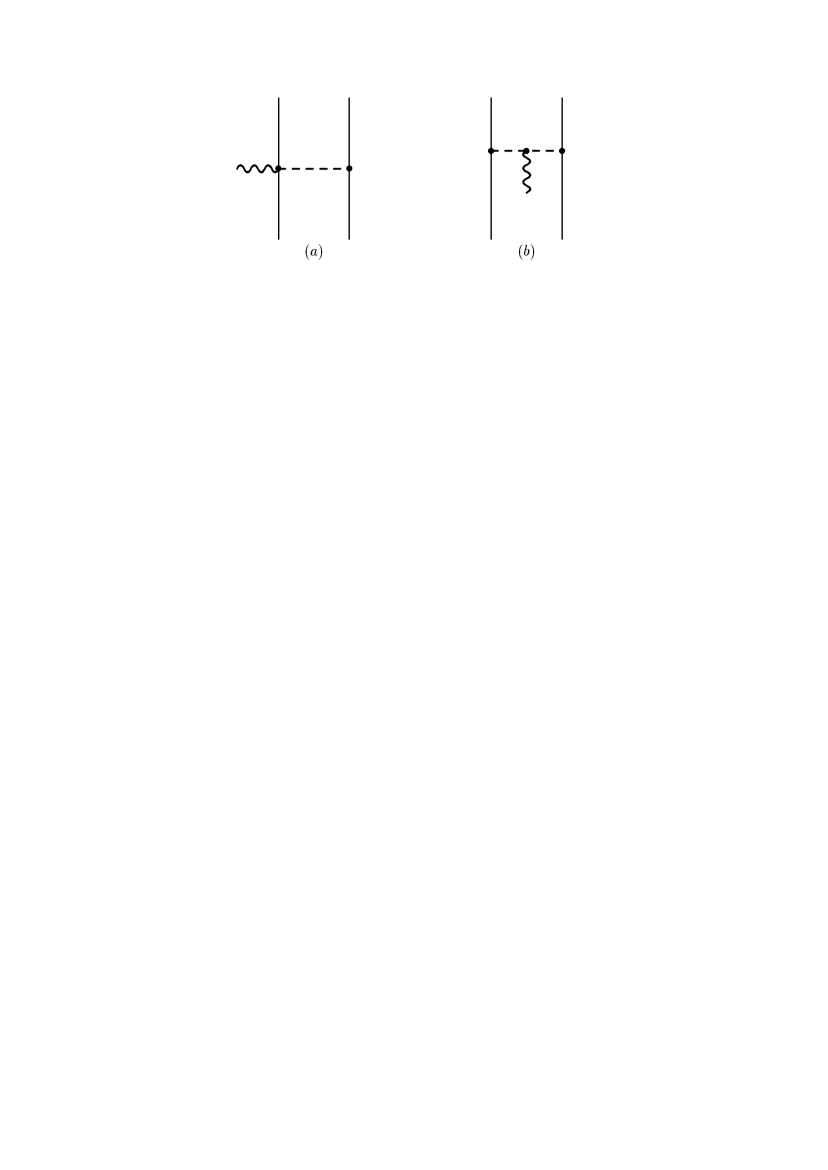
Figure 2: Tree graphs contributing to the exchange vector current, the “seagull” $(a)$ and the “pion pole” $(b)$ graph.

It follows from the counting rule eq.(5) that the leading ($O(Q^{-1}$) or $O(Q)$ relative to the impulse term) two-body currents come from the tree graphs, Fig. 2, with the vertices given by the bare ones (which will be renormalized at higher order and identified with the experimental values). Up to leading chiral order, the four-Fermi contact terms cannot contribute to the vector currents [17]. The leading two-body currents therefore are

$$V^{\mu}_{tree}(a) = i(\tau_{1}\times\tau_{2})^{z}\frac{g_{A}^{2}}{f_{\pi}^{2}}S_{1}^{\mu}\frac{S_{2}\cdot q_{2}}{m_{\pi}^{2}-q_{2}^{2}}+(1\leftrightarrow 2),$$

$$V^{\mu}_{tree}(b) = -2\,i(\tau_{1}\times\tau_{2})^{z}\frac{g_{A}^{2}}{f_{\pi}^{2}}\frac{S_{1}\cdot q_{1}}{m_{\pi}^{2}-q_{1}^{2}}\,\frac{S_{2}\cdot q_{2}}{m_{\pi}^{2}-q_{2}^{2}}\,q^{\mu}$$ (46)

where $q_{i}=p_{i}^{\prime}-p_{i}$ is the momentum transferred to the $i$th nucleon, $q_{1}^{\mu}=-q^{\mu}-\frac{1}{2}k^{\mu}$ and $q_{2}^{\mu}=q^{\mu}-\frac{1}{2}k^{\mu}$. The coupling constants and masses in the above equation are renormalized (measured) constants $g_{A}=1.257$ and $f_{\pi}=93$ MeV. The resulting MMO operator denoted ${\mbox{\boldmath$\mu$\/}}_{tree}$, is (from eqs.(46,44))

$${\mbox{\boldmath$\mu$\/}}_{tree}=e\,\frac{g_{A}^{2}m_{\pi}}{8f_{\pi}^{2}}\left\{{{\hat{T}}_{S}^{(\times)}}\left[\frac{2}{3}y_{1}(x_{\pi})-y_{0}(x_{\pi})\right]-{{\hat{T}}_{T}^{(\times)}}\,y_{1}(x_{\pi})\right\},$$ (47)

where

$$y_{0}(x) = \frac{{\mbox{e}}^{-x}}{4\pi x},$$

$$y_{1}(x) = \frac{{\mbox{e}}^{-x}}{4\pi x}(1+x)\ =\ -x\frac{d}{dx}y_{0}(x),$$

$$y_{2}(x) = \frac{{\mbox{e}}^{-x}}{4\pi x}\left(1+\frac{3}{x}+\frac{3}{x^{2}}\right)\ =\ x\frac{d}{dx}\frac{1}{x}\frac{d}{dx}y_{0}(x)$$ (48)

and

$${\hat{T}}_{S}^{(\odot)} = (\tau_{1}\odot\tau_{2})^{z}({\mbox{\boldmath$\sigma$\/}}_{1}\odot{\mbox{\boldmath$\sigma$\/}}_{2}),$$

$${\hat{T}}_{T}^{(\odot)} = (\tau_{1}\odot\tau_{2})^{z}\left[{\hat{r}}\,{\hat{r}}\cdot({\mbox{\boldmath$\sigma$\/}}_{1}\odot{\mbox{\boldmath$\sigma$\/}}_{2})-\frac{1}{3}({\mbox{\boldmath$\sigma$\/}}_{1}\odot{\mbox{\boldmath$\sigma$\/}}_{2})\right]$$ (49)

with $\odot=\pm,\,\times$. We should mention that this is the same as what one gets from the corresponding “pair” and “pionic” currents obtained in [11]. The only thing new here is its precise place in the chiral expansion.

3.2.2 Loop corrections to the one-pion-exchange currents

The first one-loop corrections corresponding to $O(Q^{2})$ relative to the leading-order tree discussed above are renormalizations of the vertices in one-pion exchange graphs. We shall first show that the corrections appear only at the ${\cal V}\pi NN$ vertex. The $\pi NN$ proper function up to one-loop accuracy is [7]

$$\Gamma_{\pi NN,i}^{a}(q)=-i\tau_{i}^{a}\frac{g_{A}}{f_{\pi}}\,q\cdot S_{i}$$ (50)

where terms proportional to $v\cdot q$ are higher-order and hence can be neglected. There are thus no one-loop corrections to the $\pi NN$ vertex. Now the Ward identity restricts the ${\cal V}\pi\pi$ proper function to the form

$$\Gamma_{{\cal V}\pi\pi}^{\mu,ab}(q_{1},q_{2}) = 2i\epsilon_{3ab}\left\{q^{\mu}+\left(q^{\mu}-\frac{k^{\mu}\,k\cdot q}{k^{2}}\right)\left[F_{\pi\pi}^{V}(k^{2})-1\right]\right\}$$ (51)

$$= 2i\epsilon_{3ab}\,q^{\mu}+{\cal O}(k^{2})$$

where $F_{\pi\pi V}^{V}(k^{2})$ is the electromagnetic form factor of the pion, $F_{\pi\pi}^{V}(k^{2})=1+{\cal O}(k^{2})$. This shows that there are no one-loop corrections from this vertex to the magnetic moment operator. Therefore we are left with the ${\cal V}\pi NN$ vertex appearing in Fig. 1$a$. Here the situation is quite analogous to the one-loop corrections in the exchange axial-charge currents [7]. The one-loop Feynman graphs contributing to the relevant vertex are given in Fig. 3.

Figure 3: One-nucleon, one-pion irreducible one-loop graphs contributing to the four-point ${\cal V}\pi NN$ vertex.

These one-loop graphs are computed in Appendix A. The result can be summarized simply as follows. The key point to underline is that for the magnetic moment operator, there are no corrections from the finite loop terms. The only contribution comes from the finite counter terms that describe the degrees of freedom that are integrated out from our low-energy effective Lagrangian. In fact there are two such terms:

$${\cal L}_{\mbox{\tiny CT}} = \frac{g_{A}^{3}\,c_{7}^{R}}{4f_{\pi}^{2}}\,{\overline{B}}\epsilon^{\mu\nu\alpha\beta}v_{\mu}\,\Delta_{\nu}^{a}\Gamma_{\alpha\beta}^{a}\,B$$ (52)

$$+ \left[\frac{i\,g_{A}\,c_{9}}{4f_{\pi}^{2}}\,{\overline{B}}\,\Delta^{a}_{\mu}{\cal P}^{\mu\nu}\Lambda_{ab}\Gamma_{\nu\alpha}^{b}S^{\alpha}\,B+\mbox{h.c.}\right]$$

where $\Gamma_{\mu\nu}=\frac{\tau_{a}}{2}\Gamma_{\mu\nu}^{a}$ and $\Delta_{\mu}=\frac{\tau_{a}}{2}\Delta_{\mu}^{a}$. Here we have defined the spin-$\frac{3}{2}$ and isospin-$\frac{3}{2}$ projection operators by

$${\cal P}^{\mu\nu}=\left(v^{\mu}v^{\nu}-g^{\mu\nu}-\frac{4}{3}S^{\mu}S^{\nu}\right),\ \ \ \ \Lambda_{ab}=\left(\delta_{ab}-\frac{\tau_{a}\tau_{b}}{3}\right).$$

The resulting one-pion exchange current, denoted $V_{1\pi}^{\mu}$, is of the form

$$V_{1\pi}^{\mu} = -i\tau_{2}^{z}\,\frac{g_{A}^{4}}{2f_{\pi}^{4}}\,c_{7}^{R}\,\frac{q_{2}\cdot S_{2}}{m_{\pi}^{2}-q_{2}^{2}}\,\epsilon^{\mu\nu\alpha\beta}v_{\nu}k_{\alpha}q_{\beta}$$ (53)

$$- \frac{g_{A}^{2}}{4f_{\pi}^{4}}\,c_{9}\,\frac{q_{2}\cdot S_{2}}{m_{\pi}^{2}-q_{2}^{2}}\,\left[\left(\frac{2}{3}\tau_{2}^{z}-\frac{i}{3}(\tau_{1}\times\tau_{2})^{z}\right)\,q_{2\beta}{\cal P}_{1}^{\beta\alpha}(k_{\alpha}\,S_{1}^{\mu}-g_{\alpha}^{\mu}\,k\cdot S_{1})\right.$$

$$\ \ \ \ \ \ \ -\ \left.\left(\frac{2}{3}\tau_{2}^{z}+\frac{i}{3}(\tau_{1}\times\tau_{2})^{z}\right)\,(S_{1}^{\mu}\,k_{\alpha}-g^{\mu}_{\alpha}\,k\cdot S_{1}){\cal P}_{1}^{\alpha\beta}q_{2\beta}\right]$$

$$+ (1\leftrightarrow 2).$$

The counter terms bring in two parameters, $c_{7}^{R}$ and $c_{9}$, to be fixed. These should be determined from experiments. Relevant experiments would be isovector pion photoproduction or radiative weak amplitudes at low energy. However, the presently available data are not accurate enough to fix the constants sufficiently reliably. The difficulty lies in the fact that those processes are dominated by the seagull term and nucleon pole term and the constants we need to fix represent small corrections that cannot be extracted from the data. We shall therefore estimate them by the resonance saturation in a way analogous to what is done for the $O(Q^{4})$ Lagrangian counter terms for $\pi\pi$ scattering [23]. The relevant resonances are the $\omega$ and $\Delta$ saturating, respectively, the constants $c_{7}^{R}$ and $c_{9}$. The results are

$${\bar{c}}_{\omega} \equiv \frac{g_{A}^{2}m_{\pi}^{2}}{f_{\pi}^{2}}\,c_{7}^{R}=\frac{g_{\omega}^{2}m_{\pi}^{2}}{8\pi^{2}g_{A}(m_{\omega}^{2}-m_{\pi}^{2})}\simeq 0.1021,$$

$${\bar{c}}_{\Delta} \equiv \frac{2m_{\pi}^{2}}{9f_{\pi}^{2}}\,c_{9}=\frac{2\,\mu_{T}\,{\cal C}\,m_{\pi}^{2}}{9g_{A}(m_{\Delta}-m_{N})m_{N}}\simeq 0.1667$$ (54)

where $g_{\omega}$ is determined from the $\omega\rightarrow\pi\gamma$ decay, $g_{\omega}=17.55$, and the $N\Delta$ transition magnetic moment $\mu_{T}$ and the $\pi N\Delta$ coupling ${\cal C}$ come from the fit to the $\Delta$ properties as explained in [24], ${\cal C}=-1.73$ and $\mu_{T}=-7.7\pm 0.5$. For details, see Appendix C. The resulting magnetic moment operator that we will use later is rather simple:

$${\mbox{\boldmath$\mu$\/}}_{1\pi}={\mbox{\boldmath$\mu$\/}}_{1\pi}^{\omega}+{\mbox{\boldmath$\mu$\/}}_{1\pi}^{\Delta}$$ (55)

with

$${\mbox{\boldmath$\mu$\/}}_{1\pi}^{\omega} = -e\,\frac{g_{A}^{2}m_{\pi}}{8f_{\pi}^{2}}{\bar{c}}_{\omega}\left\{\left({{\hat{T}}_{S}^{(+)}}+{{\hat{T}}_{S}^{(-)}}\right)\frac{{\bar{y}}_{0}(x_{\pi})}{3}+\left({{\hat{T}}_{T}^{(+)}}+{{\hat{T}}_{T}^{(-)}}\right)\,y_{2}(x_{\pi})\right\},$$

$${\mbox{\boldmath$\mu$\/}}_{1\pi}^{\Delta} = -e\,\frac{g_{A}^{2}m_{\pi}}{8f_{\pi}^{2}}{\bar{c}}_{\Delta}\left\{\left({{\hat{T}}_{S}^{(+)}}+{{\hat{T}}_{S}^{(-)}}-{{\hat{T}}_{S}^{(\times)}}\right)\frac{{\bar{y}}_{0}(x_{\pi})}{3}+\left({{\hat{T}}_{T}^{(+)}}+{{\hat{T}}_{T}^{(-)}}+\frac{1}{2}{{\hat{T}}_{T}^{(\times)}}\right)\,y_{2}(x_{\pi})\right\}.$$

This operator is equivalent to Fig. 4 calculated in the conventional meson-exchange current study. What is significant – and novel – in the context of chiral perturbation theory is that

Figure 4: Graphs that correspond to the full one-loop corrections to the one-pion-exchange graphs. These graphs plus the tree graphs are referred to as “generalized tree” graphs.

chiral symmetry constrains that there be no other contribution to the next-to-leading order one-pion exchange magnetic moment operator: There are no chiral loop corrections to the one-pion-exchange operator. This is in contrast to the case of axial-charge transitions [7] where chiral loop corrections to the one-pion exchange axial charge operator play a relatively important role. This suggests to lump all four terms of Fig. 2 and Fig. 4 together and call them “generalized tree operators”.

We should explain briefly why there are no genuine loop corrections (“chiral log terms”) here in contrast to the axial-charge operator of [7] and how the “counter terms” eq.(52) are saturated by the resonances. The genuine loop corrections arise from $q^{2}$-dependent terms where $q^{\mu}$ is the momentum transferred by the pion. Now the nucleon propagators in a loop cannot bring in a $q^{2}$-dependence because of the softness of the momentum and $v\cdot q=0$. This means that if there is any momentum-dependent term, it must arise only from the momentum dependence of the pion propagators in the loop. We see from Fig. 3 that the first seven graphs $(a-g)$ are momentum-independent and the next three graphs $(h,i,j)$ are $k^{2}$-dependent but $q^{2}$-independent. Therefore if any, chiral log terms can occur only at two-loop (or higher) order.

3.2.3 Two-pion-exchange currents

Figure 5: One-pion and one-nucleon irreducible one-loop graphs contributing to the two-body vector current. Note that one-loop graphs which contain purely nucleonic intermediate state are excluded. Only the first four graphs ($a$, $b$, $c$ and $d$) contribute to the magnetic moment operator.

There are numerous diagrams of genuine loop character that can contribute in general kinematics to the two-pion-exchange two-body current. However a drastic simplification is obtained for the magnetic moment operator in heavy-fermion formalism: only four graphs $(a)$, $(b)$, $(c)$ and $(d)$ of Fig. 5 give non-vanishing contributions to the MMO. The graph $(e)$ gives only zero-ranged operator and so will vanish in the matrix element, the graph $(f)$ is non-zero but cannot contribute to the MMO as it does not contain terms linear in $k^{\mu}$, the graph $(g)$ is identically zero because it is proportional to $v\cdot S=0$ and the remaining graphs ($(h)$, $(i)$, $(j)$, $(k)$ and $(l)$), being proportional to $v^{\mu}$, do not contribute to the space component of the vector current. The calculation of the graphs is described in Appendix B.

We pause briefly to explain why the zero-ranged graph $(e)$ does not contribute in our calculation. Such zero-ranged two-pion-exchange graphs could be divergent (that is, they could have the $\frac{1}{d-4}$ pole). This divergence can be removed by a counter term generated by ${\cal L}_{2}$, leaving us a zero-range term with a finite coefficient. As in the case of the counter terms $c_{7}^{R}$ and $c_{9}$, the (renormalized) coefficients should be fixed by experiments. However there are no experimental data, so we saturate them by resonances. As shown explicitly in Appendix C, the coefficients obtained by this procedure come out to be simply zero. This is because the only low-lying resonance that can contribute is the $\rho$-meson, but its exchange does not give rise to terms linear in $k^{\mu}$, and so gives vanishing contribution to the MMO. Even if the coefficients were non-zero, they would not contribute since short-correlations would “kill” them anyway unless the exchanged particle comes down below the chiral scale as in the case of the scalar meson in medium discussed in section 5.

The resulting two-pion exchange MMO takes the form

$${\mbox{\boldmath$\mu$\/}}_{2\pi} = -\frac{e\,m_{\pi}^{3}\,g_{A}^{2}}{256\pi^{2}f_{\pi}^{4}}\left[\frac{2}{3}\left({{\hat{T}}_{S}^{(+)}}-{{\hat{T}}_{S}^{(-)}}\right)-\left({{\hat{T}}_{T}^{(+)}}-{{\hat{T}}_{T}^{(-)}}\right)\right]\,x_{\pi}\frac{d}{dx_{\pi}}k_{0}(x_{\pi})$$ (57)

$$+ \frac{e\,m_{\pi}^{3}\,g_{A}^{4}}{256\pi^{2}f_{\pi}^{4}}\left\{\frac{2}{3}{{\hat{T}}_{S}^{(+)}}\left[-2k_{0}(x_{\pi})+4k_{1}(x_{\pi})+x_{\pi}\frac{d}{dx_{\pi}}k_{0}(x_{\pi})+2x_{\pi}\frac{d}{dx_{\pi}}k_{1}(x_{\pi})\right]\right.$$

$$\ \ \ \ \ \ \ +\ \frac{2}{3}{{\hat{T}}_{S}^{(\times)}}\left[\frac{1}{2}k_{0}(x_{\pi})-k_{1}(x_{\pi})+x_{\pi}\frac{d}{dx_{\pi}}k_{0}(x_{\pi})\right]$$

$$\ \ \ \ \ \ \ +\ {{\hat{T}}_{T}^{(+)}}\left[4k_{\rm T}(x_{\pi})-x_{\pi}\frac{d}{dx_{\pi}}k_{0}(x_{\pi})-2x_{\pi}\frac{d}{dx_{\pi}}k_{1}(x_{\pi})\right]$$

$$\left.\ \ \ \ \ \ \ +\ {{\hat{T}}_{T}^{(\times)}}\left[2k_{\rm T}(x_{\pi})-x_{\pi}\frac{d}{dx_{\pi}}k_{0}(x_{\pi})\right]\right\}$$

$$+ e\,\delta({\mbox{\boldmath$r$\/}})\left[-\frac{1}{2}G_{S}^{R}\,{{\hat{T}}_{S}^{(+)}}-\frac{1}{2}G_{A}^{R}\,{{\hat{T}}_{S}^{(-)}}-\frac{1}{8}E_{T}^{V,R}\,{{\hat{T}}_{S}^{(\times)}}\right].$$

The functions $k_{0}(x_{\pi})$, $k_{1}(x_{\pi})$ and $k_{\rm T}(x_{\pi})$ are defined by

$$k_{0}(x_{\pi}) \equiv \frac{1}{m_{\pi}^{3}}\int\frac{d^{3}{\mbox{\boldmath$q$\/}}}{(2\pi)^{3}}\,{\rm e}^{i\,{\mbox{\boldmath$q$\/}}\cdot{\mbox{\boldmath$r$\/}}}\,\int_{0}^{1}dz\,{\rm ln}\left[1+z(1-z)\frac{{\mbox{\boldmath$q$\/}}^{2}}{m_{\pi}^{2}}\right],$$

$$k_{1}(x_{\pi}) \equiv \frac{1}{m_{\pi}^{3}}\int\frac{d^{3}{\mbox{\boldmath$q$\/}}}{(2\pi)^{3}}\,{\rm e}^{i\,{\mbox{\boldmath$q$\/}}\cdot{\mbox{\boldmath$r$\/}}}\,\int_{0}^{1}dz\frac{z(1-z){\mbox{\boldmath$q$\/}}^{2}}{m_{\pi}^{2}+z(1-z){\mbox{\boldmath$q$\/}}^{2}},$$

$$k_{\rm T}(x_{\pi}) \equiv \frac{1}{m_{\pi}^{3}}x_{\pi}\frac{d}{dx_{\pi}}\frac{1}{x_{\pi}}\frac{d}{dx_{\pi}}\int\frac{d^{3}{\mbox{\boldmath$q$\/}}}{(2\pi)^{3}}\,{\rm e}^{i\,{\mbox{\boldmath$q$\/}}\cdot{\mbox{\boldmath$r$\/}}}\,\int_{0}^{1}\!\!dz\,\frac{z^{2}\,m_{\pi}^{2}}{m_{\pi}^{2}+z(1-z){\mbox{\boldmath$q$\/}}^{2}}.$$ (58)

Analytic solutions are available for nonzero $x_{\pi}$ for the functions $k_{0,1}(x_{\pi})$:

$$k_{0}(x) = -\frac{1}{\pi x^{2}}{\bf K}_{1}(2x),$$

$$\frac{d}{dx}k_{0}(x) = \frac{1}{\pi x^{2}}\left(x{\bf K}_{0}(2x)+2{\bf K}_{1}(2x)+x{\bf K}_{2}(2x)\right),$$

$$k_{1}(x) = -\frac{1}{\pi x}{\bf K}_{0}(2x),$$

$$\frac{d}{dx}k_{1}(x) = \frac{1}{\pi x}\left({\bf K}_{0}(2x)+2x{\bf K}_{1}(2x)\right)$$ (59)

where ${\bf K}_{n}(z)$ are the $n$th order modified Bessel functions.

As we explained in several places, what we have to deal with is the finite-ranged contribution. For the $n+p\rightarrow d+\gamma$ process, the contributions proportional to the ${{\hat{T}}_{S}^{(+)}}$ or ${{\hat{T}}_{T}^{(+)}}$ are zero. Dropping zero-ranged operators that vanish by short-range correlations, the MMO can be expressed in terms of the “fundamental” constants $g_{A}$ and $f_{\pi}$,

$${\mbox{\boldmath$\mu$\/}}_{2\pi} = \frac{e\,m_{\pi}^{3}\,g_{A}^{2}}{16\pi^{2}f_{\pi}^{4}}\left(\frac{2}{3}{\hat{T}}^{(-)}_{S}-{\hat{T}}^{(-)}_{T}\right)\,\int_{1}^{\infty}\!\!\!dt\,t\sqrt{t^{2}-1}\,y_{1}(2tx_{\pi})$$ (60)

$$+ \frac{e\,m_{\pi}^{3}\,g_{A}^{4}}{16\pi^{2}f_{\pi}^{4}}\int_{1}^{\infty}\!\!\!dt\,\left\{\frac{2}{3}{\hat{T}}^{(\times)}_{S}\frac{t^{3}}{\sqrt{t^{2}-1}}\left(y_{1}(2tx_{\pi})-\frac{1}{2}y_{0}(2tx_{\pi})\right)\right.$$

$$\left.\ \ \ \ \ \ \ -{\hat{T}}^{(\times)}_{T}\left(t\sqrt{t^{2}-1}\,y_{1}(2tx_{\pi})-\frac{2t^{3}-t}{\sqrt{t^{2}-1}}\,y_{2}(2tx_{\pi})\right)\right\}$$

where $x_{\pi}=m_{\pi}r$ and the functions $y$’s are defined in eq.(48).

In summary, the total magnetic moment operator up to one-loop accuracy then is

$${\mbox{\boldmath$\mu$\/}}={\mbox{\boldmath$\mu$\/}}_{\rm 1B}+{\mbox{\boldmath$\mu$\/}}_{tree}+{\mbox{\boldmath$\mu$\/}}_{1\pi}+{\mbox{\boldmath$\mu$\/}}_{2\pi}.$$ (61)

4 Application to $n+p\rightarrow d+\gamma$

4.1 A long-standing discrepancy

The radiative $np$ capture $n+p\rightarrow d+\gamma$ at threshold is the most unambiguous nuclear process where the effect of pionic currents can be clearly seen. We shall apply the magnetic moment operator derived in chiral perturbation expansion to this process.

The experimental cross-section measured accurately with the neutrons of thermal velocity, $v_{n}=2200\ \mbox{m/sec}$, is [25]

$$\sigma_{\rm{exp}}=(334.2\pm 0.5)\ \mbox{mb}.$$ (62)

We first describe the prediction made in impulse approximation. For this, we note that the process involves very low energy, the relative momentum in the center of mass system being

$$p=\frac{1}{2}m_{{}_{\rm N}}v_{n}\simeq 3.4451\times 10^{-3}\ \mbox{MeV}\simeq\left(5.7278\times 10^{4}\ \mbox{fm}\right)^{-1}$$ (63)

where the nucleon mass $m_{{}_{\rm N}}$ is defined by twice the reduced mass of the proton and neutron, $m_{{}_{\rm N}}=2m_{p}m_{n}/(m_{p}+m_{n})\simeq 938.92$ MeV. At this extremely low energy, the process is predominantly governed by the isovector M1 transition operator. We write the wavefunctions of the initial ${}^{1}S_{0}$ $np$ state and the final deuteron state, respectively, by

$$\Psi_{np}({\mbox{\boldmath$r$\/}}) = \frac{1}{\sqrt{4\pi}\,r}\,u_{0}(r)\,\chi_{00}\,\zeta_{10},$$

$$\Psi_{d}({\mbox{\boldmath$r$\/}};J_{z}) = \frac{1}{\sqrt{4\pi}\,r}\left[u(r)+\frac{w(r)}{\sqrt{8}}\,S_{12}({\hat{r}})\right]\,\chi_{1J_{z}}\,\zeta_{00}$$ (64)

where $\chi_{JJ_{z}}$ ($\zeta_{TT_{z}}$) is the spin (isospin) spinor and

$$S_{12}(\hat{r})\equiv 3\,{\mbox{\boldmath$\sigma$\/}}_{1}\cdot{\hat{r}}\ {\mbox{\boldmath$\sigma$\/}}_{2}\cdot{\hat{r}}-{\mbox{\boldmath$\sigma$\/}}_{1}\cdot{\mbox{\boldmath$\sigma$\/}}_{2}.$$ (65)

The radial functions $u_{0}(r)$ and $u(r)$ are normalized so that their large-$r$ asymptotic functions $\phi_{0}(r)$ and $\phi(r)$ have $\phi_{0}(0)=\phi(0)=1$. We have

$$\lim_{r\rightarrow\infty}u_{0}(r) = \phi_{0}(r)\equiv\frac{\sin(pr+\delta_{s})}{\sin(\delta_{s})}\simeq 1-\frac{r}{a_{s}},$$ (66)

$$\lim_{r\rightarrow\infty}u(r) = \phi(r)\equiv{\mbox{e}}^{-\gamma r},$$

$$\lim_{r\rightarrow\infty}w(r) = \eta\,{\mbox{e}}^{-\gamma r}\left(1+\frac{3}{\gamma r}+\frac{3}{(\gamma r)^{2}}\right)$$ (67)

where $\eta$ is the $D/S$ ratio, $\gamma=\sqrt{B_{d}m_{{}_{\rm N}}}\simeq 45.702\ \mbox{MeV}\simeq(4.3177\ \mbox{fm})^{-1}$, $B_{d}\simeq 2.2246$ MeV is the deuteron binding energy, $a_{s}\simeq-23.749\ \mbox{fm}$ is the singlet $np$ scattering length and $\delta_{s}$ is the ${}^{1}S_{0}$ $np$ phase shift. In terms of the M1 transition matrix $M$ defined by

$$\frac{e}{2m_{p}}M\equiv\int\!\!d^{3}{\mbox{\boldmath$r$\/}}\,\,\Psi_{np}^{\dagger}({\mbox{\boldmath$r$\/}})\left[{\mbox{\boldmath$\mu$\/}}({\mbox{\boldmath$r$\/}})\right]^{z}\Psi_{d}({\mbox{\boldmath$r$\/}};0),$$ (68)

the cross section can be written as

$$\sigma=G\,M^{2},\ \ \ \ \ G\equiv\frac{e^{2}\omega^{3}\,A_{s}^{2}\,a_{s}^{2}}{4\,v_{n}\,m_{p}^{2}}$$ (69)

where $v_{n}$ is the neutron velocity, $\omega\simeq B_{d}$ is the energy of the emitted photon, and $A_{s}\simeq 0.8846\ \mbox{fm}^{-1/2}$ is the normalization factor of the deuteron wavefunction,

$$\frac{1}{A_{s}^{2}}\equiv\int\!\!d^{3}{\mbox{\boldmath$r$\/}}\,\,\Psi_{d}^{\dagger}({\mbox{\boldmath$r$\/}})\Psi_{d}({\mbox{\boldmath$r$\/}};0)=\int_{0}^{\infty}\!\!dr\,\left[\,u^{2}(r)+w^{2}(r)\right].$$ (70)

Now the transition matrix $M_{\rm 1B}$ for the one-body magnetic moment operator (45) is

$$M_{\rm 1B}=\mu_{V}\,\int_{0}^{\infty}\!\!dr\,u_{0}(r)u(r).$$ (71)

Austern showed in 1953 [26] that $M_{\rm 1B}$ can be estimated accurately in an effective-range expansion in terms of low energy parameters. The leading contribution is

$$M_{0}\equiv\mu_{V}\,\int_{0}^{\infty}\!\!dr\,\phi_{0}(r)\phi(r)=\frac{\mu_{V}}{\gamma}\,\left(1-\frac{1}{\gamma\,a_{s}}\right).$$ (72)

The next order contribution in the effective range expansion can also be represented [26] by scattering lengths, effective ranges and the $D$-wave probability of deuteron. The impulse approximation obtained with this method comes out to be $\sigma_{imp}(\mbox{Austern})=(303\pm 4)\ \mbox{mb}$. As we will explain in the following subsection, one can obtain a considerably more accurate value with the Argonne $v_{18}$ potential [27],

$$\sigma_{imp}=305.6\ \mbox{mb}.$$ (73)

The discrepancy between the impulse (73) (or rather the Austern result) and the experiment (62) had been a long-standing puzzle in nuclear physics until Riska and Brown [9] supplied in 1972 the missing 10 % contribution in terms of meson-exchange currents. In the following subsection, we will do an accurate one-loop chiral perturbation calculation, using the Argonne $v_{18}$ potential.

4.2 Exchange current contribution

In calculating the matrix element of the two-body currents $M_{\rm 2B}$, it is convenient to perform the angular integration first and evaluate the spin-isospin matrix elements for various spin-isospin operators:

$$\langle{\hat{T}}_{S,T}^{(\odot)}\rangle_{\rm SS} = \int\!\frac{d\Omega}{4\pi}\,\left(\chi_{00}\,\zeta_{10}\right)^{\dagger}\left[{\hat{T}}_{S,T}^{(\odot)}\right]^{z}\chi_{10}\,\zeta_{00},$$

$$\langle{\hat{T}}_{S,T}^{(\odot)}\rangle_{\rm SD} = \int\!\frac{d\Omega}{4\pi}\,\left(\chi_{00}\,\zeta_{10}\right)^{\dagger}\left[{\hat{T}}_{S,T}^{(\odot)}\right]^{z}\,S_{12}(\hat{r})\chi_{10}\,\zeta_{00}.$$ (74)

It is straightforward to show that

$$\langle{{\hat{T}}_{S}^{(-)}}\rangle_{\rm SS}=\langle{{\hat{T}}_{S}^{(\times)}}\rangle_{\rm SS}=4,\ \ \ \ \ \ \langle{{\hat{T}}_{T}^{(-)}}\rangle_{\rm SD}=\langle{{\hat{T}}_{T}^{(\times)}}\rangle_{\rm SD}=-\frac{16}{3}$$ (75)

and that all others are equal to zero. The resulting two-body transition matrix elements are

$$M_{\rm 2B}=M_{\rm 2B}^{\rm SS}+M_{\rm 2B}^{\rm SD}$$ (76)

with

$$M_{\rm 2B}^{\rm SS} = \frac{g_{A}^{2}\,m_{p}\,m_{\pi}}{f_{\pi}^{2}}\,\int_{0}^{\infty}\!\!dr\,u_{0}(r)\,u(r)\,\left[f_{S}^{(-)}(x_{\pi})+f_{S}^{(\times)}(x_{\pi})\right],$$

$$M_{\rm 2B}^{\rm SD} = -\frac{\sqrt{2}g_{A}^{2}\,m_{p}\,m_{\pi}}{3f_{\pi}^{2}}\,\int_{0}^{\infty}\!\!dr\,u_{0}(r)\,w(r)\,\left[f_{T}^{(-)}(x_{\pi})+f_{T}^{(\times)}(x_{\pi})\right]$$ (77)

where the functions $f_{S,T}^{(-,\times)}(x_{\pi})$ are ($x_{\pi}\equiv m_{\pi}\,r$)

$$f_{S}^{(-)}(x_{\pi}) = -\frac{{\bar{c}}_{\omega}+{\bar{c}}_{\Delta}}{3}\,y_{0}(x_{\pi})+\frac{m_{\pi}^{2}}{48\pi^{2}f_{\pi}^{2}}\,x_{\pi}\frac{d}{dx_{\pi}}k_{0}(x_{\pi})+\frac{4f_{\pi}^{2}}{g_{A}^{2}m_{\pi}}G_{A}^{R}\delta({\mbox{\boldmath$r$\/}}),$$

$$f_{S}^{(\times)}(x_{\pi}) = \frac{{\bar{c}}_{\Delta}}{3}y_{0}(x_{\pi})+\left[\frac{2}{3}y_{1}(x_{\pi})-y_{0}(x_{\pi})\right]$$

$$+ \frac{g_{A}^{2}\,m_{\pi}^{2}}{48\pi^{2}f_{\pi}^{2}}\left[\frac{1}{2}k_{0}(x_{\pi})-k_{1}(x_{\pi})+x_{\pi}\frac{d}{dx_{\pi}}k_{0}(x_{\pi})\right]+\frac{4f_{\pi}^{2}}{g_{A}^{2}m_{\pi}}E_{T}^{V,R}\delta({\mbox{\boldmath$r$\/}}),$$

$$f_{T}^{(-)}(x_{\pi}) = -({\bar{c}}_{\omega}+{\bar{c}}_{\Delta})\,y_{2}(x_{\pi})-\frac{m_{\pi}^{2}}{32\pi^{2}f_{\pi}^{2}}\,x_{\pi}\frac{d}{dx_{\pi}}k_{0}(x_{\pi}),$$

$$f_{T}^{(\times)}(x_{\pi}) = -\frac{{\bar{c}}_{\Delta}}{2}\,y_{2}(x_{\pi})+\frac{g_{A}^{2}\,m_{\pi}^{2}}{32\pi^{2}f_{\pi}^{2}}\left[2k_{\rm T}(x_{\pi})-x_{\pi}\frac{d}{dx_{\pi}}k_{0}(x_{\pi})\right].$$ (78)

4.3 The $\Delta$ degree of freedom

So far, we have not considered the $\Delta$ degrees of freedom explicitly. It figured indirectly only as a resonance that saturates one of the counter terms. The role of the $\Delta$ is subtle because of the non-commutativity of the large-$N_{c}$ limit and the chiral limit. The matter is simple if the mass gap, $\delta m=m_{\Delta}-m_{{}_{\rm N}}$, is either small enough to be regarded as ${\cal O}(Q)$ or large enough to be regarded as ${\cal O}(\Lambda_{\chi})$. In the large-$N_{c}$ limit, $\delta m={\cal O}(N_{c}^{-1})$ is to be taken to be smaller than $m_{\pi}={\cal O}(N_{c}^{0})$. On the other hand, in the chiral limit, it is to be taken to be bigger than $m_{\pi}$ since it remains finite when $m_{\pi}$ goes to zero. In reality, neither is a good approximation. For the process we are considering, we believe that both approaches, one with the $\delta m$ treated as small (referred to as “type-I”) and the other with the $\delta m$ treated as heavy (referred to as “type-II”) could be employed equally well.

In the type-I approach, we should treat the nucleon and the $\Delta$ on the same footing. Then the counting rule should be modified to

$$\nu^{\rm I}=4-2C-\left(\frac{E_{N}+E_{\Delta}}{2}+E_{H}+E_{E}\right)+2L+\sum_{i}{\bar{\nu}}^{\rm I}_{i},\ \ \ \ \ {\bar{\nu}}^{\rm I}_{i}\equiv d_{i}+\frac{n_{i}+n_{i}^{*}}{2}+h_{i}+e_{i}-2$$ (79)

where $E_{\Delta}$ is the number of external $\Delta$ lines and $n_{i}^{*}$ the number of $\Delta$ lines attached to the $i$th vertex. In this approach, we cannot integrate out the $\Delta$ degree of freedom without introducing non-locality in the effective Lagrangian. This also means that the $\Delta$ must be included in the “reducible graphs” or in terms of Schrödinger picture, in the wavefunctions. This procedure has often been used in nuclear physics calculations for processes that involve the excitation of the $\Delta$ resonance. Processes involving large energy transfer are better treated in this manner.

In the type-II approach, we should be able to treat $\delta m$ as heavy, say, $\delta m={\cal O}(Q^{0})$. In this case, we cannot attach any $Q$-factor to the propagator, since $1/(\delta m-v\cdot k)\sim 1/\delta m={\cal O}(Q^{0})$. The counting rule in this case is

$$\nu^{\rm II}=4-2C-\left(\frac{E_{N}}{2}+E_{\Delta}+E_{H}+E_{E}\right)+2L+\sum_{i}{\bar{\nu}}^{\rm II}_{i},\ \ \ \ \ {\bar{\nu}}^{\rm II}_{i}\equiv d_{i}+\frac{n_{i}}{2}+n_{i}^{*}+h_{i}+e_{i}-2.$$ (80)

If this applies, we can freely integrate out the $\Delta$ degree of freedom as well as other massive degrees of freedom. This will be the case for the process we are considering. As shown recently by Mallik [28], this approach is equivalent to the type-I approach in certain kinematics (such as in our case). It appears that the type-I approach is more general in the sense that it can be applied to a wide range of kinematical conditions whereas the type II is restricted. For our case, the type-II approach is much simpler. This can be seen as follows. Since the energy carried by the exchanged pion (since the photon is thermal) is small compared with the $N\Delta$ mass difference, the $\Delta$ propagator in tree graphs may be safely expanded as

$$\frac{1}{\delta m-v\cdot k}=\frac{1}{\delta m}+\frac{v\cdot k}{(\delta m)^{2}}+\cdots,$$ (81)

where $v\cdot k$ corresponds to the energy of the pion or the photon. In our one-loop calculation, only the first term is retained. How good is this approximation? In general, the $\Delta$ propagator in the two-pion-exchange graphs may carry an arbitrary loop momentum. The only constraint we have is that the loop momentum be of order of the characteristic momentum, $Q$. In our process, however, the characteristic momentum involved is $\gamma=\sqrt{B_{d}\,m_{{}_{\rm N}}}\simeq 45$ MeV. Therefore the error involved in truncating the series (81) is at most of order $\gamma/(\delta m)\simeq 0.15$ in the two-pion-exchange contributions. Since the overall two-pion-exchange contribution to the thermal neutron process is very small, as we shall find below, this is a safe approximation.

4.4 Numerical results

To calculate the capture cross section, we need accurate two-nucleon wavefunctions. This is because we need to have an accurate prediction for ${}^{1}S_{0}$ $np$ scattering length, $a_{s}$, to which the cross section is directly proportional. (There is also an implicit $a_{s}$-dependence through the wavefunction.) A majority of nuclear potentials fail to reproduce the experimental value $a_{s}^{exp}=-23.749\pm 0.008$ fm, because they do not fully incorporate the charge-independence-breaking (CIB) effect of the potential. It is not enough to incorporate the Coulomb interactions and the mass difference between the charged and neutral pions. It is also necessary to incorporate the CIB effects in intermediate- and short-range potentials. Potentials which do not account for such CIB effects predict typically $\sim a_{s}\sim-17$ fm. For example, Reid’s hard core potential [29] predicts $a_{s}(\mbox{Reid})=-16.7$ fm, giving a poor impulse approximation result for the capture rate, $\sigma_{\rm imp}(\mbox{Reid})=173.7$ mb to be compared with what is needed, $\sim 306$ mb (see (82)). A similar result is obtained with the Reid soft core potential, the Paris potential etc. An important point to note is that the ratios $\delta$ of the matrix elements of the exchange currents to the impulse current are remarkably insensitive to the potentials, as we shall discuss later.

We take the Argonne $v_{18}$ potential recently constructed by Wiringa, Stoks and Schiavilla [27]. This potential is fit to 1787 $pp$ and 2514 $np$ scattering data in the range 0–350 MeV with an excellent $\chi^{2}$ of 1.09 and gives the deuteron properties – the asymptotic S-state normalization, $A_{S}$, the $D/S$ ratio, $\eta$, and the deuteron radius, $d_{d}$ – close to the experimental values. Electromagnetic properties also come out well, modulo exchange-current and relativistic corrections. It predicts $a_{s}^{th}=-23.732$ fm in excellent agreement with the experimental value $a_{s}^{{exp}}=-23.749\pm 0.008$ fm. The single-particle matrix element with this potential gives the impulse approximation cross section (given by ${\mbox{\boldmath$\mu$\/}}_{tree}$ of eq.(61))

$$\sigma_{imp}=305.6\ \mbox{mb},$$ (82)

$\sim$9.6% less than the experimental value $\sigma_{exp}=334.2\pm 0.5$ mb.

Figure 6: Total capture cross section $\sigma_{\rm cap}$ (top) and $\delta$’s (bottom) vs. the cut-off $r_{c}$. The solid line represents the total contributions and the experimental values are given by the shaded band indicating the error bar. The dotted line gives $\delta_{\rm tree}$, the dashed line $\delta_{\rm tree}+\delta_{1\pi}^{\Delta}$, the dot-dashed line $\delta_{\rm tree}+\delta_{1\pi}=\delta_{\rm tree}+\delta_{1\pi}^{\Delta}+\delta_{1\pi}^{\omega}$ and the solid line the total ratio, $\delta_{\rm 2B}$.

$r_{c}(\mbox{fm})$	0.1	0.2	0.3	0.4	0.5	0.6	0.7	Reid
$\sigma$(mb)	336.1	336.0	335.7	335.2	334.4	333.3	331.8	188.8
$\delta_{tree}$ (%)	2.608	2.608	2.609	2.609	2.605	2.592	2.563	2.577
$\delta_{1\pi}^{\omega}$ (%)	0.435	0.431	0.423	0.408	0.382	0.346	0.301	0.367
$\delta_{1\pi}^{\Delta}$ (%)	1.364	1.355	1.334	1.294	1.228	1.132	1.011	1.168
$\delta_{1\pi}$ (%)	1.799	1.786	1.757	1.702	1.610	1.477	1.311	1.535
$\delta_{2\pi}$ (%)	0.471	0.457	0.443	0.424	0.397	0.362	0.319	0.319
$\delta_{\rm 2B}$ (%)	4.878	4.851	4.809	4.745	4.612	4.431	4.193	4.431

Table 2: The total cross section $\sigma$ and the $\delta$’s calculated with the Argonne $v_{18}$ potential. The $\delta$’s are defined by $\delta_{x}=M_{x}/M_{\rm 1B}\times 100$ % for a given $x$, $\delta_{1\pi}=\delta_{1\pi}^{\omega}+\delta_{1\pi}^{\Delta}$, and $\delta_{\rm 2B}=\delta_{\rm tree}+\delta_{1\pi}+\delta_{2\pi}$. The last column shows the results with the Reid hard-core potential.

	$SS$	$SD$	Sum ($SS+SD$)
$\delta_{tree}$ (%)	1.534	1.071	2.605
$\delta_{1\pi}^{\omega}$ (%)	$-0.119$	0.501	0.382
$\delta_{1\pi}^{\Delta}$ (%)	0	1.228	1.228
$\delta_{1\pi}$ (%)	$-0.119$	1.729	1.610
$\delta_{2\pi}$ (%)	0.449	$-0.052$	0.397
$\delta_{\rm 2B}$ (%)	1.864	2.748	4.612

Table 3: The $\delta$’s with $r_{c}=0.5$ fm calculated with the Argonne $v_{18}$ potential.

In computing the matrix elements of the two-body operators, we need to take into account short-range correlations in the wavefunctions. Short-range correlations must involve nucleon interactions at a length scale less than the scale given by chiral symmetry breaking and cannot be accounted for by low-order chiral perturbation expansions. In calculating Feynman diagrams of ChPT, the cut-off of the theory is incorporated in the regularization. Therefore nuclear wavefunctions do not incorporate the effect of the degrees of freedom that are cut off from the theory and the short-range correlation that is represented by a hard-core radius is missing. We do not know how to implement this effect in a way consistent with the strategy of ChPT. In this paper as in [7], we account for the short-range effect simply by multiplying the integrand of the radial integral by $\theta(r-r_{c})$,

$$\int_{0}^{\infty}\!\!dr\rightarrow\int_{r_{c}}^{\infty}\!\!dr\,.$$

This procedure is justified by the insensitivity of the result to the hard-core size.

We use the physical values for masses and constants that appear in the theory. There are no unknown parameters other than the short-range cutoff parameter $r_{c}$. The resulting total cross section is plotted and compared with the experiment [25] in Fig. 6 (top) for a wide range of $r_{c}$, $0<r_{c}\mathrel{\raise 1.29167pt\hbox{$<$\kern-7.5pt\lower 4.30554pt\hbox{$\sim$}}}0.7$ fm. Figure 6 (bottom) shows the contribution of each term in terms of the ratios $\delta_{tree}\equiv M_{tree}/M_{\rm 1B}$, $\delta_{1\pi}\equiv M_{1\pi}/M_{\rm 1B}$, $\delta_{2\pi}\equiv M_{2\pi}/M_{\rm 1B}$ and $\delta_{2B}$ which is the sum. For $\delta_{1\pi}$, we divided it into two part, $\delta_{1\pi}^{\omega}$ and $\delta_{1\pi}^{\Delta}$. The ratio corresponding to the “generalized tree” contributions is $\delta_{\rm GTO}=\delta_{tree}+\delta_{1\pi}$. These ratios are plotted in Figure 6 (bottom). We also list the total cross section and the ratios in Table 2 and 3. In Table 2, the results are listed for varying $r_{c}$’s. The last column shows the results with Reid’s hard-core potential [29]. Notice that, although the cross section is very sensitive to the potential, the ratios are essentially the same. This confirms that the ratios are highly model-independent, a conclusion reached previously. We should also point out that the $r_{c}$ which gives approximately the same result with Reid’s potential is $r_{c}\simeq 0.6$ fm to be compared with the hard-core radius of the Reid potential, $0.55$ fm. In Table 3, we decompose the ratios into the $SS$ and $SD$ channels (where $SS$ ($SD$) denotes the contribution to the $S$-wave ($D$-wave) of the deuteron wavefunction) for a fixed $r_{c}$, $r_{c}=0.5$ fm. The intrinsic uncertainty associated with short-distance physics notwithstanding, the theoretical prediction

$$\sigma_{th}=334\pm 3\ \mbox{mb}$$ (83)

(where the theoretical error bar represents only the dependence on the hard-core cut-off) is in remarkable agreement with the experiment, say, within less than 1% ! We have checked that the isoscalar moment contribution to the process is totally negligible.

4.5 The chiral-filter phenomenon

One of the principal results in our calculation is that the “generalized tree” contributions dominate to the N²L order, with only a small correction (less than 0.6 % of the single-particle matrix element) coming from the genuine one-loop correction. This agrees with the “chiral filter” mechanism seen in the axial-charge transitions [7] and confirms the conjecture made in [12]. We should make a few additional remarks on this point.

It is interesting to compare the M1 transition (thermal neutron capture) with the axial-charge transitions [7]. In fact, the meaning of “chiral filter” is slightly different in the two : In axial-charge transitions, the chiral filter mechanism is reflected in the smallness of the loop contribution compared with the tree contribution whereas in M1 processes, it is in the suppression of the two-pion exchange (one-loop) term compared with the total one-pion exchange (generalized tree) contribution. If we denote the operator by ${\cal M}^{A}$ (${\cal M}^{V}$) and its matrix element by $M^{A}$ ($M^{V}$) for axial-charge (M1) transitions, then the statement is

$$M_{loop}^{A} = M_{1\pi}^{A}+M_{2\pi}^{A}\ll M_{tree}^{A},$$ (84)

$$M_{2\pi}^{V} \ll M_{GTO}^{V}=M_{tree}^{V}+M_{1\pi}^{V}.$$ (85)

These two observations can be unified if one accepts that what chiral filter conjecture really says is that the long-range operator (characterized by its tail ${\mbox{e}}^{-m_{\pi}r}$) dominates whenever it is not suppressed by kinematical or symmetry reasons. In the axial-charge transition case, as was discussed in [7], the ${\cal M}_{1\pi}^{A}$ can be decomposed into two parts, long-ranged and short-ranged as

$${\cal M}_{1\pi}^{A}=\delta_{soft}{\cal M}_{tree}^{A}+{\cal M}_{1\pi;short}^{A}$$ (86)

with

$$\delta_{soft}=c_{3}^{R}\frac{m_{\pi}^{2}}{f_{\pi}^{2}}+\frac{m_{\pi}^{2}}{16\pi^{2}f_{\pi}^{2}}\left[\frac{1+3g_{A}^{2}}{2}\left(2-\frac{\pi}{\sqrt{3}}\right)-(1+2g_{A}^{2})\left(\frac{17}{9}-\frac{\pi}{\sqrt{3}}\right)\right]\simeq 0.051$$ (87)

where ${\cal M}_{1\pi;short}^{A}$ represents the short-range contribution (shorter-ranged compared to one-pion-exchange) and the counter term $c_{3}^{R}$ is given by the charge radius of the proton. In [7], we showed that $\delta_{soft}$ (or $c_{3}^{R}$) could be understood in terms of the $\rho$-meson degree of freedom. Since two-pion-exchange contributions are short-ranged, we can clearly divide the exchange axial-vector current into a long-ranged component and a residual short-ranged part:

$${\cal M}_{long}^{A} = (1+\delta_{soft}){\cal M}_{tree}^{A},$$

$${\cal M}_{short}^{A} = {\cal M}_{1\pi;short}^{A}+{\cal M}_{2\pi}^{A}.$$ (88)

Put in this form, the chiral filter effect is even more transparent and striking

$$\left[\frac{M_{short}}{M_{long}}\right]^{A}\simeq(0.03-0.05)$$ (89)

with the matter density ranging $0<\rho<\rho_{0}$. In the M1 transition in question, the corresponding long- and short-ranged operators are

$${\cal M}_{long}^{V} = {\cal M}_{tree}^{V}+{\cal M}_{1\pi;\omega}^{V}+{\cal M}_{1\pi;\Delta}^{V}={\cal M}_{GTO},$$

$${\cal M}_{short}^{V} = {\cal M}_{2\pi}^{V}.$$ (90)

We see that in this extended form the chiral filter works equally well for both processes.

5 The BR Scaling

There is very little understanding of the meaning of the short-distance correlation cut-off $r_{c}$ in the context of ChPT. As discussed in [7], the loop terms contain zero-range operators in coordinate space. In addition, four-Fermi counter terms in the chiral Lagrangian with unknown constants are of contact interaction. At higher chiral order, increasingly shorter-ranged operators would enter together with the zero-ranged ones. Now if we were able to compute nuclear interactions to all orders in chiral perturbation theory, the delta functions in the current would be naturally regularized and would cause no problem. Such a calculation of course is an impossible feat. The practical application of chiral perturbation theory is limited to low orders in the chiral expansion, so a cut-off would be needed to screen the interactions shorter-ranged than accessible by the chiral expansion adopted. This means that all interactions of range shorter than the inverse chiral scale $\sim 1\ {\mbox{GeV}}^{-1}$ should not contribute as additional operators. Clearly such a calculation would be meaningful only if the dependence on the cut-off were weak. Our calculation here meets that criterion. In the present work, we find that the $r_{c}$-dependence is trivially small over wide range, $0<r_{c}\mathrel{\raise 1.29167pt\hbox{$<$\kern-7.5pt\lower 4.30554pt\hbox{$\sim$}}}0.5$ fm, and the theoretical prediction agrees exactly with the experiment at $r_{c}\simeq 0.5$ fm. The $r_{c}$-independence and the success can be traced to the fact that there is no relevant low-energy resonances which contribute to the counter terms associated with four-Fermi interactions and the fact that the short-range correlation effect is automatically included in the $np$ and deuteron wavefunctions.

There appear subtleties, however, when nuclear density goes up, as in the case of the axial-charge transitions in heavy nuclei studied elsewhere. As nuclear density increases, some of the massive degrees of freedom that have been integrated out could come down in energy as suggested by Brown and Rho[14, 15]. If the mass comes down below the relevant chiral scale, roughly equivalent to $r_{c}^{-1}$, then the short-range correlation can no longer suppress such a contribution. We shall now suggest that this is what happens with a scalar “dilaton” field.

Consider the scalar field $\chi$ associated with the trace anomaly of QCD exploited in [14, 15]. In matter-free space ($\rho\approx 0$), the scalar field, associated with scalar glueball, is massive with a mass $m_{\chi}\sim 2\ {\mbox{GeV}}>m_{\rho}$, so may be integrated out. A simple calculation shows that this leads to an $O(Q^{3})$ four-Fermi counter-term Lagrangian of the form

$$\Delta{\cal L}={\alpha}({\overline{B}}B)\left({\overline{B}}\Gamma_{1/m}B\right)$$ (91)

where $\alpha$ is a dimension–4 constant and $\Gamma_{1/m}$ is the operator which appears in $1/m_{{}_{\rm N}}$ expansion, eq.(28),

$$\Gamma_{1/m}=-D^{2}+(v\cdot D)^{2}+S^{\mu\nu}\Gamma_{\mu\nu}+g_{A}^{2}(v\cdot\Delta)^{2}+2g_{A}\left\{v\cdot\Delta,S\cdot D\right\}+\cdots.$$

One can see from dimensional counting that this Lagrangian is highly “irrelevant” and hence would be negligible. However the situation can be drastically different in medium. As discussed in [15], a low-lying excitation with the quantum number of scalar meson exists in dense medium. Such a “dilaton” is supposed to play an important role in nuclear physics as manifested in Walecka’s theory with a low-lying scalar meson and also required by a “mended symmetry” emerging at a higher energy-momentum scale [30]. What this means is that instead of the zero-range interaction coming from the four-Fermi interaction, we would have a finite-range interaction with the range determined by the scalar mass in medium, $m^{\star}_{\sigma}$ where $\sigma$ is the scalar corresponding to the dilaton. We can gain a simple idea by noting that the Lagrangian (91) can be obtained from the “$1/m_{{}_{\rm N}}$” Lagrangian (27) by replacing the nucleon mass by its effective operator,

$$m_{{}_{\rm N}}\rightarrow m_{{}_{\rm N}}^{*}=m_{{}_{\rm N}}\left(1+\kappa\frac{{\overline{B}}B}{\rho_{0}}\right)^{-1}$$ (92)

where $\rho_{0}$ is the normal nuclear matter density and $\kappa$ is a constant. If one assumes that $\kappa$ is saturated by the $\sigma$ meson effective in medium [15], then one finds

$$\kappa=\frac{g_{\sigma}^{2}\,\rho_{0}}{m_{{}_{\rm N}}\,m_{\sigma}^{2}}$$ (93)

where $g_{\sigma}$ is the $\sigma NN$ coupling and $m_{\sigma}$ the $\sigma$ mass. In mean-field approximation, (91) and (93) give, for $m_{\sigma}\approx 600{\mbox{MeV}}$ and $g_{\sigma}\approx 10$, a substantial enhancement to the one-body axial charge operator as well as to the one-body isovector magnetic moment operator:

$$\frac{\delta_{\sigma}A^{0}}{A^{0}}=\frac{\delta_{\sigma}{\mbox{\boldmath$\mu$\/}}}{{\mbox{\boldmath$\mu$\/}}}=\kappa\,\frac{\rho}{\rho_{0}}\simeq 0.4\ \frac{\rho}{\rho_{0}}.$$ (94)

This is basically the enhancement in the axial charge in heavy nuclei as found in phenomenological models with a low-lying scalar meson by Towner [31] and by Kirchbach et al  [32]. It is equivalent to the Brown-Rho scaling $f_{\pi}^{\star}/f_{\pi}\approx m_{N}^{\star}/m_{N}$ as discussed in [33].

6 Conclusion

This paper provides a chiral symmetry interpretation of the long-standing exchange-current result of Riska and Brown. It supports the chiral-filter argument verified in the axial-charge transitions and offers yet another evidence that chiral Lagrangians figure importantly in nuclear physics.

Here as well as in [7], ChPT is developed in the long wavelength regime where the expansion makes sense. The question remains as to at what point the expansion of ChPT breaks down. In particular, the meaning of short-range correlation remains to be clarified, an issue which cannot be ignored in any nuclear process. An intriguing question in this connection is posed by the observation that the generalized one-pion exchange process dominates even in $e+d\rightarrow n+p+e^{\prime}$ at a large momentum transfer[1]. The only way one can understand this phenomenon would be that the chiral filter takes place even to large momentum transfers. It would be interesting to verify this in a systematic chiral perturbation calculation.

Another intriguing problem is the role of many-body interactions from chiral symmetry point of view. We know that for processes involving small energy transfers, three-body and other higher-body currents are suppressed. But this will not be the case for non-negligible energy transfers. There multi-body currents will certainly become important. Furthermore as nuclear density increases (i.e., heavy nuclei or nuclear matter), particle masses can drop below the characteristic chiral mass scale and introduce density-dependent renormalization in the parameters of the chiral Lagrangian. We have illustrated this with BR scaling [14] but the basic issue can be more general in the sense that it involves relevant and irrelevant degrees of freedom as the length scale is varied. This problem needs further study.

Acknowledgments

We thank the Institute for Nuclear Theory at the University of Washington for its hospitality and the Department of Energy for partial support during the completion of this work. The work of TSP and DPM is supported in part by the Korea Science and Engineering Foundation through the Center for Theoretical Physics of Seoul National University and in part by the Korea Ministry of Education under the grant No.BSRI-94-2418.

Appendices

A Renormalization of the ${\cal V}\pi NN$ vertex

Consider the ${\cal V}\pi NN$ vertex ${\Gamma_{\pi V}^{\mu,ab}}(k,q)$ defined by the kinematics

$$N(m_{{}_{\rm N}}v)\rightarrow N(m_{{}_{\rm N}}v-k-q)+\pi_{b}(q)+{\cal V}_{a}(k).$$

Restricting ourselves to on-shell nucleons (i.e., $v\cdot(k+q)=0$) and including the $1/m_{{}_{\rm N}}$ corrections, the vertex has the form

$${\Gamma_{\pi V}^{\mu,ab}} = -\epsilon_{abc}\tau_{c}\frac{g_{A}}{f_{\pi}}\,S^{\mu}$$ (A.1)

$$+ \epsilon_{abc}\tau_{c}\left[-\frac{g_{A}}{f_{\pi}^{3}}S^{\mu}y\,h_{0}^{A}(y)+\frac{g_{A}^{3}}{f_{\pi}^{3}}v^{\mu}\frac{d-3}{4}q\cdot S\,h_{4}^{A}(y)-\frac{g_{A}}{f_{\pi}^{3}}y\,I_{A}^{\mu}(k)\right]$$

$$+ i\delta_{ab}\left[2\frac{g_{A}}{f_{\pi}^{3}}S^{\mu}y\,h_{0}^{S}(y)-\frac{3}{4}\frac{g_{A}^{3}}{f_{\pi}^{3}}v^{\mu}\,q\cdot S\,h_{4}^{S}(y)-2\frac{g_{A}}{f_{\pi}^{3}}y\,I_{S}^{\mu}(k)-2\frac{g_{A}^{3}}{f_{\pi}^{3}}q_{\nu}I^{\mu\nu}(k)\right]$$

$$+ \frac{v\cdot q}{2m_{{}_{\rm N}}f_{\pi}}\,S^{\mu}\,\left[i\delta_{ab}\,(g_{A}+b_{3})+\epsilon_{abc}\tau_{c}\,b_{5}\right]$$

$$+ {\Gamma_{\pi V,\mbox{\tiny CT}}^{\mu,ab}}$$

where ${\Gamma_{\pi V,\mbox{\tiny CT}}^{\mu,ab}}$ are the contributions from the counter-term Lagrangian, $y=v\cdot k$ and $h_{0,4}^{A,S}(y)=\frac{1}{2}\left[h_{0,4}(y)\mp h_{0,4}(-y)\right]$ which were given explicitly in [7]. The functions $I_{A,S}^{\mu}(k)=\frac{1}{2}\left[I^{\mu}(k)\mp I^{\mu}(-k)\right]$ and $I^{\mu\nu}(k)$ are defined by

$$I^{\mu}(k) = \int_{l}\frac{S\cdot l\,(2l+k)^{\mu}}{v\cdot l\,(l^{2}-M^{2})\,\left[(l+k)^{2}-M^{2}\right]},$$

$$I^{\mu\nu}(k) = \int_{l}\frac{S\cdot(l+k)\,S^{\nu}\,S\cdot l\,(2l+k)^{\mu}}{v\cdot(l+k)\,v\cdot l\,(l^{2}-M^{2})\,\left[(l+k)^{2}-M^{2}\right]}$$ (A.2)

where

$$\int_{l}\equiv\frac{\mu^{4-d}}{i}\int\!\!\frac{d^{d}l}{(2\pi)^{d}},$$

$d=4-2\epsilon$ is the spacetime dimension and $\mu$ is the renormalization scale. For small momentum, they can be simplified to

$$I^{\mu}(k) = -\frac{m_{\pi}}{8\pi}\,S^{\mu}-\left(S^{\mu}\,v\cdot k+v^{\mu}\,S\cdot k\right)\eta+{\cal O}(k^{2}),$$

$$I^{\mu\nu}(k) = -\frac{m_{\pi}}{32\pi}v^{\mu}\,S^{\nu}-\frac{i}{4}\epsilon^{\mu\nu\alpha\beta}v_{\alpha}k_{\beta}\eta+{\cal O}(k^{2})$$ (A.3)

where ${\cal O}(k^{2})$ denotes terms equal to, or higher than, second order in $k^{\mu}$ and $\epsilon_{0123}=1$. With $v\cdot k=0$, they become

$$I^{\mu}(k) = -v^{\mu}\,S\cdot k\,f_{0}(k^{2})$$

$$- \frac{1}{16\pi}\int_{0}^{1}dz\left(2S^{\mu}\sqrt{m_{\pi}^{2}-z(1-z)k^{2}}+q^{\mu}\,S\cdot q\,\frac{z(2z-1)}{\sqrt{m_{\pi}^{2}-z(1-z)k^{2}}}\right),$$

$$I^{\mu\nu}(k) = -\frac{i}{4}\epsilon^{\mu\nu\alpha\beta}v_{\alpha}k_{\beta}f_{0}(k^{2})$$ (A.4)

$$- \frac{v^{\mu}}{8\pi}\left(\frac{1}{4}S^{\nu}+2S\cdot k\,S^{\nu}\,S\cdot k\frac{\partial}{\partial k^{2}}\right)\int_{0}^{1}dz\sqrt{m_{\pi}^{2}-z(1-z)k^{2}}$$

where $f_{0}$ is [7]

$$f_{0}(q^{2}) = \eta-\frac{1}{16\pi^{2}}K_{0}(q^{2})$$ (A.5)

and the divergent quantity $\eta$ is defined in eq.(34).

All the divergences in eq.(A.1) can be removed by the counter-term Lagrangian (38), that is, the terms with $c$’s, whose contribution to the ${\cal V}\pi NN$ vertex is

$${\Gamma_{\pi V,\mbox{\tiny CT}}^{\mu,ab}} = \epsilon_{abc}\tau_{c}\left[-\frac{g_{A}}{2f_{\pi}^{3}}\,c_{2}\,q\cdot S\,v^{\mu}\,v\cdot k+\frac{g_{A}}{2f_{\pi}^{3}}c_{8}v\cdot q\left(v^{\mu}\,k\cdot S-S^{\mu}\,v\cdot k\right)\right]$$ (A.6)

$$+ i\delta_{ab}\left[i\frac{g_{A}^{3}}{2f_{\pi}^{3}}c_{7}\epsilon^{\mu\nu\alpha\beta}v_{\alpha}k_{\beta}q_{\nu}\right]$$

$$- \frac{i\,g_{A}}{4f_{\pi}^{3}}\,c_{9}\,\left[\Lambda_{ba}\,q_{\beta}{\cal P}^{\beta\alpha}(k_{\alpha}\,S^{\mu}-g_{\alpha}^{\mu}\,k\cdot S)-\Lambda_{ab}\,(S^{\mu}\,k_{\alpha}-g^{\mu}_{\alpha}\,k\cdot S){\cal P}^{\alpha\beta}q_{\beta}\right]$$

with

$$c_{2} = \frac{d-3}{3}g_{A}^{2}\eta+c_{2}^{R},$$

$$c_{7} = -\eta+c_{7}^{R},$$

$$c_{8} = 2\eta+c_{8}^{R}.$$ (A.7)

Here $c_{i}^{R}$ are finite, $\mu$-independent renormalized constants. When $v\cdot k=v\cdot q=0$ we have a simpler expression:

$${\Gamma_{\pi V}^{\mu,ab}}(k,q) = -\epsilon_{abc}\tau_{c}\frac{g_{A}}{f_{\pi}}S^{\mu}-\delta_{ab}\frac{g_{A}^{3}}{2f_{\pi}^{3}}\epsilon^{\mu\nu\alpha\beta}v_{\alpha}k_{\beta}q_{\nu}\left[f_{0}(k^{2})-f_{0}(0)+c_{7}^{R}\right]$$

$$- \frac{i\,g_{A}}{4f_{\pi}^{3}}\,c_{9}\,\left[\Lambda_{ba}\,q_{\beta}{\cal P}^{\beta\alpha}(k_{\alpha}\,S^{\mu}-g_{\alpha}^{\mu}\,k\cdot S)-\Lambda_{ab}\,(S^{\mu}\,k_{\alpha}-g^{\mu}_{\alpha}\,k\cdot S){\cal P}^{\alpha\beta}q_{\beta}\right].$$

Terms proportional to $v^{\mu}$ do not figure in our calculation and so are omitted. Note that the above equation is finite and $\mu$-independent and contains two parameters, $c_{7}^{R}$ and $c_{9}$ which were fixed in our calculation by resonance saturation.

B Renormalization of two-pion-exchange contributions

The two-body vector currents come from the two-pion exchange graphs and one-pion exchange graphs with a four-Fermi contact vertex (see Figure 5):

$$J_{\!\rm em}^{\mu}(a) = -(2\tau_{2}-i\tau_{1}\times\tau_{2})^{z}\frac{g_{A}^{2}}{4f_{\pi}^{4}}\,S_{1}^{\mu}\,S_{1}\cdot q_{2}\,f_{0}(q_{2}^{2})$$

$$+ (2\tau_{2}+i\tau_{1}\times\tau_{2})^{z}\,\frac{g_{A}^{2}}{4f_{\pi}^{4}}\,S_{1}\cdot q_{2}\,S_{1}^{\mu}\,f_{0}(q_{2}^{2})+(1\leftrightarrow 2),$$

$$J_{\!\rm em}^{\mu}(b) = -(2\tau_{2}-i\tau_{1}\times\tau_{2})^{z}\,\frac{g_{A}^{2}}{2f_{\pi}^{4}}\,\int_{l}\frac{S_{1}\,\cdot(l-q_{1})\,S_{1}\cdot l\,(2l+q_{2}-q_{1})^{\mu}}{(l^{2}-m_{\pi}^{2})\,\left[(l-q_{1})^{2}-m_{\pi}^{2}\right]\left[(l+q_{2})^{2}-m_{\pi}^{2}\right]}$$

$$- (2\tau_{2}+i\tau_{1}\times\tau_{2})^{z}\,\frac{g_{A}^{2}}{2f_{\pi}^{4}}\,\int_{l}\frac{S_{1}\cdot l\,S_{1}\,\cdot(l+q_{1})\,(2l+q_{1}-q_{2})^{\mu}}{(l^{2}-m_{\pi}^{2})\,\left[(l+q_{1})^{2}-m_{\pi}^{2}\right]\left[(l-q_{2})^{2}-m_{\pi}^{2}\right]}$$

$$\ +\ (1\leftrightarrow 2),$$

$$J_{\!\rm em}^{\mu}(c) = -(2\tau_{1}+2\tau_{2}-i\tau_{1}\times\tau_{2})^{z}\,\frac{g_{A}^{4}}{f_{\pi}^{4}}\,S_{1}^{\mu}S_{1}^{\alpha}S_{2}^{\beta}S_{2}^{\nu}\,F_{\alpha\beta\nu}(q_{2})$$

$$- (2\tau_{1}+2\tau_{2}-i\tau_{1}\times\tau_{2})^{z}\,\frac{g_{A}^{4}}{f_{\pi}^{4}}\,S_{1}^{\nu}S_{1}^{\alpha}S_{2}^{\beta}S_{2}^{\mu}\,F_{\alpha\beta\nu}(-q_{1})+(1\leftrightarrow 2),$$

$$J_{\!\rm em}^{\mu}(d) = (2\tau_{1}+2\tau_{2}-i\tau_{1}\times\tau_{2})^{z}\,\frac{g_{A}^{4}}{f_{\pi}^{4}}\,\otimes$$

$$\ \int_{l}\frac{S_{1}\cdot(l-q_{1})\,S_{1}\cdot l\,S_{2}\cdot l\,S_{2}\cdot(l+q_{2})\,(2l+q_{2}-q_{1})^{\mu}}{(v\cdot l)^{2}\,(l^{2}-m_{\pi}^{2})\,\left[(l-q_{1})^{2}-m_{\pi}^{2}\right]\,\left[(l+q_{2})^{2}-m_{\pi}^{2}\right]}+(1\leftrightarrow 2),$$

$$J_{\!\rm em}^{\mu}(e) = -2i\epsilon^{3bc}\,\frac{g_{A}^{2}}{f_{\pi}^{2}}\,\sum_{A}C_{A}\int_{l}\frac{S_{1}\cdot\left(l+\frac{k}{2}\right)\ \tau_{1}^{b}\Gamma_{1}^{A}\tau_{1}^{c}\ S_{1}\cdot\left(l-\frac{k}{2}\right)\ \Gamma_{2}^{A}\ l^{\mu}}{(v\cdot l)^{2}\left[\left(l-\frac{k}{2}\right)^{2}-m_{\pi}^{2}\right]\,\left[\left(l+\frac{k}{2}\right)^{2}-m_{\pi}^{2}\right]}$$

$$\ +\ (1\leftrightarrow 2),$$

$$J_{\!\rm em}^{\mu}(f) = -i(\tau_{1}\times\tau_{2})^{z}\,\frac{1}{4f_{\pi}^{4}}\,\int_{l}\frac{(v\cdot l)^{2}\,(2l+q_{2}-q_{1})^{\mu}}{(l^{2}-m_{\pi}^{2})\,\left[(l-q_{1})^{2}-m_{\pi}^{2}\right]\,\left[(l+q_{2})^{2}-m_{\pi}^{2}\right]},$$

$$J_{\!\rm em}^{\mu}(g) \propto v\cdot S\,S^{\mu}\,=\,0$$ (B.1)

where

$$F_{\alpha\beta\nu}(q) = \int_{l}\frac{l_{\alpha}\,l_{\beta}\,(l+q)_{\nu}}{(v\cdot l)^{2}\,(l^{2}-m_{\pi}^{2})\,\left[(l+q_{2})^{2}-m_{\pi}^{2}\right]}$$ (B.2)

$$= \frac{1}{2}\left(g_{\alpha\nu}q_{\beta}+g_{\beta\nu}q_{\alpha}-g_{\alpha\beta}q_{\nu}\right)f_{0}(q^{2})+\frac{1}{16\pi^{2}}K_{1}(q^{2})\frac{q_{\alpha}q_{\beta}q_{\nu}}{-q^{2}}+(\mbox{$v$'s}).$$

Here and in what follows, ($v$’s) generically stands for terms proportional to $v_{\alpha},\ v_{\beta}$ or $v_{\nu}$. The function $f_{0}(q^{2})$ was defined in eq.(A.5) and the $K_{1}(q^{2})$ was given in [7],

$$K_{0}(q^{2}) = \int_{0}^{1}\!\!dz\,\ln\left[1-z(1-z)\frac{q^{2}}{m_{\pi}^{2}}\right],$$

$$K_{1}(q^{2}) = \int_{0}^{1}\!\!dz\,\frac{-z(1-z)q^{2}}{m_{\pi}^{2}-z(1-z)q^{2}}.$$ (B.3)

Since for the M1 transitions, it is sufficient to retain only the terms linear in $k$, we define

$$J_{\!\rm em}^{\mu,\nu}\equiv\left.\frac{\partial J_{\!\rm em}^{\mu}}{\partial k_{\nu}}\right|_{k=0}\,.$$ (B.4)

A direct calculation leads to

$$J_{\!\rm em}^{\mu,\nu}(b) = -J_{\!\rm em}^{\nu,\mu}(a),$$

$$J_{\!\rm em}^{\mu,\nu}(d) = -J_{\!\rm em}^{\nu,\mu}(c)+\delta J_{\!\rm em}^{\mu,\nu}(d)$$ (B.5)

with

$$\delta J_{\!\rm em}^{\mu,\nu}(d)=-(2\tau_{1}+2\tau_{2}-i\tau_{1}\times\tau_{2})^{z}\,\frac{g_{A}^{4}}{2f_{\pi}^{4}}\left(S_{1}^{\mu}S_{1}^{\alpha}S_{2}^{\beta}S_{2}^{\nu}-S_{1}^{\nu}S_{1}^{\alpha}S_{2}^{\beta}S_{2}^{\mu}\right)F_{\alpha\beta}(q)+(1\leftrightarrow 2)$$ (B.6)

and

$$F_{\alpha\beta}(q) = \int_{l}\frac{l_{\alpha}\,l_{\beta}}{(v\cdot l)^{2}\,(l^{2}-m_{\pi}^{2})\,\left[(l+q)^{2}-m_{\pi}^{2}\right]}$$ (B.7)

$$= -g_{\alpha\beta}f_{0}(q^{2})+\frac{q_{\alpha}q_{\beta}}{8\pi^{2}}\int_{0}^{1}dz\,\frac{z^{2}}{m_{\pi}^{2}-z(1-z)q^{2}}+(\mbox{$v$'s})$$

where ($v$’s) denotes terms proportional to $v_{\alpha}$ or $v_{\beta}$.

The divergencies appearing in the one-loop graphs, eq.(B.1), are removed by the counter-term contribution coming from the terms with $G$’s and $E_{T}^{V}$ in the counter-term Lagrangian eq.(38). Summing up all the two-pion-exchange and counter-term contributions, we have

$$J_{\!\rm em}^{\mu,\nu}(2\pi) = \left\{\frac{g_{A}^{2}}{4f_{\pi}^{4}}\frac{\partial}{\partial q_{\nu}}\left(\tau_{2}^{z}\left[S_{1}^{\mu},\ S_{1}\cdot q\right]\,{\bar{f}}_{0}(q^{2})\right)\right.$$ (B.8)

$$+ \left.(2\tau_{1}+2\tau_{2}-i\tau_{1}\times\tau_{2})^{z}\frac{g_{A}^{4}}{2f_{\pi}^{4}}\left(\frac{\partial}{\partial q_{\nu}}{\bar{F}}_{1}^{\mu}(S_{1},S_{2};\,q)-S_{1}^{\mu}S_{1}^{\alpha}S_{2}^{\beta}S_{2}^{\nu}{\bar{F}}_{\alpha\beta}(q)\right)\right\}$$

$$- (\mu\leftrightarrow\nu)\ +(1\leftrightarrow 2)$$

$$+ J_{\rm finite}^{\mu,\nu}(2\pi)$$

where

$${\bar{F}}_{1}^{\mu}(S_{1},S_{2};\,q) = \left(S_{1}^{\mu}S_{1}^{\alpha}S_{2}^{\beta}S_{2}^{\nu}-S_{1}^{\nu}S_{1}^{\alpha}S_{2}^{\beta}S_{2}^{\mu}\right)\ {\bar{F}}_{\alpha\beta\nu}(q),$$

$${\bar{F}}_{\alpha\beta\nu}(q) = -\frac{1}{32\pi^{2}}\left(g_{\alpha\nu}q_{\beta}+g_{\beta\nu}q_{\alpha}-g_{\alpha\beta}q_{\nu}\right)K_{0}(q^{2})+\frac{1}{16\pi^{2}}K_{1}(q^{2})\frac{q_{\alpha}q_{\beta}q_{\nu}}{-q^{2}}+(\mbox{$v$'s}),$$

$${\bar{F}}_{\alpha\beta}(q) = \frac{g_{\alpha\beta}}{16\pi^{2}}K_{0}(q^{2})+\frac{q_{\alpha}q_{\beta}}{8\pi^{2}}\int_{0}^{1}dz\,\frac{z^{2}}{m_{\pi}^{2}-z(1-z)q^{2}}+(\mbox{$v$'s})$$ (B.9)

and $J_{\rm finite}^{\mu,\nu}(2\pi)$ is the sum of the divergent part of the loop graphs and the counter-term contribution,

$$J_{\rm finite}^{\mu,\nu}(2\pi) = G_{S}^{R}\,(\tau_{1}+\tau_{2})^{z}\left(S_{1}^{\mu\nu}+S_{2}^{\mu\nu}\right)-G_{A}^{R}\,(\tau_{1}-\tau_{2})^{z}\left(S_{1}^{\mu\nu}-S_{2}^{\mu\nu}\right)$$ (B.10)

$$- \frac{i}{2}\,E_{T}^{V,R}\,(\tau_{1}\times\tau_{2})^{z}\,\left(S_{1}^{\mu\alpha}S^{\nu}_{2\alpha}-S_{1}^{\nu\alpha}S^{\mu}_{2\alpha}\right).$$

C Resonance-exchange contributions

In this appendix, we write down an effective chiral Lagrangian that contains the $\Delta(1232)$ and vector mesons ($\rho^{\mu}$ and $\omega^{\mu}$) in addition to $\pi$ and $N$ and apply it to the exchange currents. Instead of writing a Lagrangian with all low-lying resonances in full generality, we shall write only those terms relevant to nuclear processes which can be compared with successful phenomenological model Lagrangians employed in nuclear physics. (The axial field $a_{1}$ can be incorporated readily but we will not consider here.)

In heavy fermion formalism, including the “$1/m_{{}_{\rm N}}$” terms, the relevant Lagrangian is

$${\cal L}^{\rm res} = {\overline{B}}\left(iv\cdot{\cal D}+2g_{A}\,S\cdot i\Delta\right)B+f_{\pi}^{2}{\mbox{Tr}}(i\Delta_{\mu}\,i\Delta^{\mu})+\frac{f_{\pi}^{2}}{4}m_{\pi}^{2}{\mbox{Tr}}(\Sigma+\Sigma^{\dagger})$$ (C.1)

$$+ \frac{1}{2m_{{}_{\rm N}}}{\overline{B}}\left(-{\cal D}^{2}+(v\cdot{\cal D})^{2}-g_{A}^{2}(v\cdot i\Delta)^{2}-2ig_{A}\left\{v\cdot i\Delta,S\cdot{\cal D}\right\}\right)B$$

$$- \frac{i}{2m_{{}_{\rm N}}}{\overline{B}}\left(g_{\rho}\mu_{\rm V}[S^{\mu},S^{\nu}]\rho_{\mu\nu}+\frac{g_{\omega}}{2}\mu_{\rm S}[S^{\mu},S^{\nu}]\omega_{\mu\nu}\right)B$$

$$+ m_{\rho}^{2}{\mbox{Tr}}\!\left(\rho_{\mu}-\frac{1}{g_{\rho}}i\Gamma_{\mu}\right)^{2}+\frac{1}{2}m_{\omega}^{2}\left(\omega_{\mu}-\frac{2}{g_{\omega}}{\cal B}_{\mu}\right)^{2}-\frac{1}{2}{\mbox{Tr}}\,(\rho_{\mu\nu}\rho^{\mu\nu})-\frac{1}{4}\omega_{\mu\nu}\omega^{\mu\nu}$$

$$+ {\cal L}_{\Delta}+{\cal L}_{an}$$

with ${\cal D}_{\mu}=\partial_{\mu}-ig_{\rho}\rho_{\mu}-\frac{i}{2}g_{\omega}\omega_{\mu}$, $\rho_{\mu\nu}=\partial_{\mu}\rho_{\nu}-\partial_{\nu}\rho_{\mu}-ig_{\rho}\left[\rho_{\mu},\rho_{\nu}\right]$,

$${\cal L}_{\Delta}={\bar{T}}_{\mu}\left(\delta m_{\!\Delta}-iv\cdot{\cal D}\right)T^{\mu}+\left[{\bar{T}}^{\mu}\left(-{\cal C}\,i\Delta_{\mu}-i\frac{g_{\rho}\mu_{\rm T}}{2m_{{}_{\rm N}}}\rho_{\mu\nu}S^{\nu}\right)B+\,\mbox{h.\,c.}\right]$$ (C.2)

and

$${\cal L}_{an}=g_{\omega\rho\pi}\epsilon^{\mu\nu\alpha\beta}{\vec{\pi}}\cdot\partial_{\mu}{\vec{\rho}}_{\nu}\partial_{\alpha}\omega_{\beta}+\cdots$$ (C.3)

In (C.2), $\delta m_{\!\Delta}=m_{\Delta}-m_{{}_{\rm N}}\simeq 293$ MeV, ${\bar{T}}XT\equiv{\bar{T}}_{jkl}X^{j}_{m}T^{mkl}$ and ${\bar{T}}XB\equiv{\bar{T}}_{jkl}X^{j}_{m}B^{k}\,\epsilon^{3lm}$. From the $\Delta$ decay width, we get ${\cal C}=-1.73$. The value of $\mu_{\rm T}$ has been determined [24] to be $\mu_{\rm T}=-7.7\pm 0.5$. The anomalous parity term (C.3) is the same as in [34] with

$$g_{\omega\rho\pi}=-\frac{g_{\rho}g_{\omega}}{8\pi^{2}f_{\pi}}.$$ (C.4)

The ellipsis stands for anomalous parity terms that are irrelevant in our calculation.

We determine $g_{\rho}$ by the KSRF relation, $m_{\rho}^{2}=2g_{\rho}^{2}f_{\pi}^{2}$ or $g_{\rho}\simeq 5.85$, and $g_{\omega}$ by assuming the ideal mixing, $g_{\omega}=3g_{\rho}\simeq 17.55$. To see how good the anomalous parity Lagrangian is, consider the decay widths of $\omega\rightarrow\pi\gamma$ and $\rho\rightarrow\pi\gamma$. Our Lagrangian predicts

$$\Gamma(\omega\rightarrow\pi\gamma) = \frac{\alpha}{24}\left|\frac{g_{\omega\rho\pi}}{g_{\rho}}\right|^{2}\,m_{\omega}^{3}\left(1-\frac{m_{\pi}^{2}}{m_{\omega}^{2}}\right)^{3}\simeq 0.758\ \mbox{MeV},$$ (C.5)

$$\Gamma(\rho\rightarrow\pi\gamma) = \frac{\alpha}{24}\left|\frac{g_{\omega\rho\pi}}{g_{\omega}}\right|^{2}\,m_{\rho}^{3}\left(1-\frac{m_{\pi}^{2}}{m_{\rho}^{2}}\right)^{3}\simeq 0.080\ \mbox{MeV},$$ (C.6)

which are in reasonable agreement the experimental values [35], $\Gamma^{\rm{exp}}(\omega\rightarrow\pi\gamma)=0.717\pm 0.050$ MeV, $\Gamma^{\rm{exp}}(\rho^{\pm}\rightarrow\pi^{\pm}\gamma)=0.068\pm 0.007$ MeV and $\Gamma^{\rm{exp}}(\rho^{0}\rightarrow\pi^{0}\gamma)=0.121\pm 0.031$ MeV.

The characteristics of this Lagrangian can be summarized as follows:

• It has chiral symmetry and other symmetries consistent with low-energy QCD.

• It respects the vector-meson dominance, universality etc. and satisfies the KSRF relation.

• The chiral Lagrangian containing pions and nucleons only are recovered if the $m_{\rho}$ and $m_{\omega}$ masses are taken to infinity.

From the Lagrangian (C.1), one sees that only six graphs given in Fig. 7 can make non-zero contributions to the vector current, other graphs being either of order ${\cal O}(m_{{}_{\rm N}}^{-2})$ or vanishing.

Figure 7: Graphs that contribute to the two-body vector currents.

They have simple physical interpretations. Figure 7$a$ is the seagull graph with no form factors since $a_{1}$-meson is absent. Figure 7$b$ is the “pionic graph” with a form factor associated with the $\rho$-meson dominance. Figures 7$c$ and 7$d$ stem from ${\cal L}_{an}$, with Figure 7$d$ contributing to the baryonic current. Figure 7$e$ is new: although it gives a non-vanishing short-ranged Sachs moment, it cannot contribute to the $\mu$ in two-body systems. Finally, Figure 7$f$ is a $\Delta$-resonance contribution. The explicit forms of the currents derived from these graphs are:

$$J_{\!\rm em}^{\mu}(a) = i(\tau_{1}\times\tau_{2})^{z}\frac{g_{A}^{2}}{f_{\pi}^{2}}S_{1}^{\mu}\frac{S_{2}\cdot q_{2}}{m_{\pi}^{2}-q_{2}^{2}}+(1\leftrightarrow 2),$$

$$J_{\!\rm em}^{\mu}(b) = -2\,i(\tau_{1}\times\tau_{2})^{z}\frac{g_{A}^{2}}{f_{\pi}^{2}}\frac{m_{\rho}^{2}}{m_{\rho}^{2}-k^{2}}\,\frac{S_{1}\cdot q_{1}}{m_{\pi}^{2}-q_{1}^{2}}\,\frac{S_{2}\cdot q_{2}}{m_{\pi}^{2}-q_{2}^{2}}\,\left(q^{\mu}-\frac{k^{\mu}\,k\cdot q}{m_{\rho}^{2}}\right),$$

$$J_{\!\rm em}^{\mu}(c) = -i\tau_{2}^{z}\,\frac{g_{A}}{16\pi^{2}f_{\pi}^{2}}\,\frac{m_{\rho}^{2}}{m_{\rho}^{2}-k^{2}}\,\frac{g_{\omega}^{2}}{m_{\omega}^{2}-q_{1}^{2}}\,\frac{q_{2}\cdot S_{2}}{m_{\pi}^{2}-q_{2}^{2}}\,\epsilon^{\mu\nu\alpha\beta}v_{\nu}k_{\alpha}q_{\beta}+(1\leftrightarrow 2),$$

$$J_{\!\rm em}^{\mu}(d) = -i\,\tau_{1}\cdot\tau_{2}\,\frac{g_{A}}{16\pi^{2}f_{\pi}^{2}}\,\frac{m_{\omega}^{2}}{m_{\omega}^{2}-k^{2}}\,\frac{g_{\rho}^{2}}{m_{\rho}^{2}-q_{1}^{2}}\,\frac{q_{2}\cdot S_{2}}{m_{\pi}^{2}-q_{2}^{2}}\,\epsilon^{\mu\nu\alpha\beta}v_{\nu}k_{\alpha}q_{\beta}+(1\leftrightarrow 2),$$

$$J_{\!\rm em}^{\mu}(e) = -i(\tau_{1}\times\tau_{2})^{z}\frac{g_{\rho}^{2}}{2}\,\frac{m_{\rho}^{2}}{m_{\rho}^{2}-k^{2}}\,\frac{1}{m_{\rho}^{2}-q_{1}^{2}}\,\frac{1}{m_{\rho}^{2}-q_{2}^{2}}\,\left(q^{\mu}-\frac{k^{\mu}\,k\cdot q}{m_{\rho}^{2}}\right),$$

$$J_{\!\rm em}^{\mu}(f) = -\frac{\mu_{\rm T}\,{\cal C}\,g_{A}}{4m_{{}_{\rm N}}\,\delta m_{\!\Delta}\,f_{\pi}^{2}}\,\frac{q_{2}\cdot S_{2}}{m_{\pi}^{2}-q_{2}^{2}}\,\left[\left(\frac{2}{3}\tau_{2}^{z}-\frac{i}{3}(\tau_{1}\times\tau_{2})^{z}\right)\,q_{2\beta}{\cal P}_{1}^{\beta\alpha}(k_{\alpha}\,S_{1}^{\mu}-g_{\alpha}^{\mu}\,k\cdot S_{1})\right.$$ (C.7)

$$\ \ \ \ -\ \left.\left(\frac{2}{3}\tau_{2}^{z}+\frac{i}{3}(\tau_{1}\times\tau_{2})^{z}\right)\,(S_{1}^{\mu}\,k_{\alpha}-g^{\mu}_{\alpha}\,k\cdot S_{1}){\cal P}_{1}^{\alpha\beta}q_{2\beta}\right]+(1\leftrightarrow 2),$$

where the projection operator ${\cal P}_{1}^{\alpha\beta}$ is defined by

$${\cal P}_{1}^{\alpha\beta}=v^{\alpha}v^{\beta}-g^{\alpha\beta}-\frac{4}{3}S_{1}^{\alpha}S_{1}^{\beta}.$$

We have dropped terms of order ${\cal O}(m_{{}_{\rm N}}^{-2})$ and order $v^{\mu}\cdot{\cal O}(m_{{}_{\rm N}}^{-1})$, while keeping terms up to ${\cal O}(m_{{}_{\rm N}}^{-1})$ for the space component and up to ${\cal O}(m_{{}_{\rm N}}^{0})$ for the time component. The corresponding magnetic operators then take the form

$${\mbox{\boldmath$\mu$\/}}(a) = e\,\frac{g_{A}^{2}m_{\pi}}{16f_{\pi}^{2}}\left(\frac{2}{3}{{\hat{T}}_{S}^{(\times)}}-{{\hat{T}}_{T}^{(\times)}}\right)\,y_{1}(x_{\pi}),$$

$${\mbox{\boldmath$\mu$\/}}(b) = e\,\frac{g_{A}^{2}m_{\pi}}{16f_{\pi}^{2}}\left(\frac{2}{3}{{\hat{T}}_{S}^{(\times)}}\left[y_{1}(x_{\pi})-3y_{0}(x_{\pi})\right]-{{\hat{T}}_{T}^{(\times)}}\,y_{1}(x_{\pi})\right),$$

$${\mbox{\boldmath$\mu$\/}(c)} = -\frac{e\,g_{A}}{64\pi^{2}f_{\pi}^{2}}\,\frac{g_{\omega}^{2}}{m_{\omega}^{2}-m_{\pi}^{2}}\left(\frac{1}{3}\left({{\hat{T}}_{S}^{(+)}}+{{\hat{T}}_{S}^{(-)}}\right)\left[m_{\pi}^{3}\,y_{0}(x_{\pi})-m_{\omega}^{3}\,y_{0}(m_{\omega}r)\right]\right.$$

$$\left.\ \ \ \ \ \ \ \ +\ \left({{\hat{T}}_{T}^{(+)}}+{{\hat{T}}_{T}^{(-)}}\right)\,\left[m_{\pi}^{3}\,y_{2}(x_{\pi})-m_{\omega}^{3}\,y_{2}(m_{\omega}r)\right]\right),$$

$${\mbox{\boldmath$\mu$\/}}(d) = -\frac{e\,g_{A}}{32\pi^{2}f_{\pi}^{2}}\,\frac{g_{\rho}^{2}}{m_{\rho}^{2}-m_{\pi}^{2}}\left(\frac{1}{3}B_{\rm S}^{(+)}\left[m_{\pi}^{3}\,y_{0}(x_{\pi})-m_{\rho}^{3}\,y_{0}(m_{\rho}r)\right]\right.$$

$$\left.\ \ \ \ \ \ \ \ +\ B_{\rm T}^{(+)}\,\left[m_{\pi}^{3}\,y_{2}(x_{\pi})-m_{\rho}^{3}\,y_{2}(m_{\omega}r)\right]\right),$$

$${\mbox{\boldmath$\mu$\/}}(e) = 0,$$

$${\mbox{\boldmath$\mu$\/}}(f) = -\frac{e\,\mu_{\rm T}\,{\cal C}\,g_{A}\,m_{\pi}^{3}}{36m_{{}_{\rm N}}\,\delta m_{\!\Delta}\,f_{\pi}^{2}}\left(\frac{1}{3}\left({{\hat{T}}_{S}^{(+)}}+{{\hat{T}}_{S}^{(-)}}-{{\hat{T}}_{S}^{(\times)}}\right){\bar{y}}_{0}(x_{\pi})\right.$$ (C.8)

$$\left.\ \ \ \ \ \ +\ \left({{\hat{T}}_{T}^{(+)}}+{{\hat{T}}_{T}^{(-)}}+\frac{1}{2}{{\hat{T}}_{T}^{(\times)}}\right)y_{2}(x_{\pi})\right)$$

where ${\bar{y}}_{0}(x)=y_{0}(x)-\delta({\mbox{\boldmath$x$\/}})$ and

$$B_{\rm S}^{(+)} \equiv \tau_{1}\cdot\tau_{2}\ ({\mbox{\boldmath$\sigma$\/}}_{1}+{\mbox{\boldmath$\sigma$\/}}_{2}),$$

$$B_{\rm T}^{(+)} \equiv \tau_{1}\cdot\tau_{2}\ \left[{\hat{r}}\ {\hat{r}}\cdot({\mbox{\boldmath$\sigma$\/}}_{1}+{\mbox{\boldmath$\sigma$\/}}_{2})-\frac{1}{3}({\mbox{\boldmath$\sigma$\/}}_{1}+{\mbox{\boldmath$\sigma$\/}}_{2})\right].$$ (C.9)

As emphasized in the main text, the short-ranged contribution ${\mbox{\boldmath$\mu$\/}}(e)$ (i.e., the four-Fermi contact term) is equal to zero.

References

• [1] B. Frois and J.-F. Mathiot, Comments Part. Nucl. Phys. 18 (1989) 291.
• [2] M. Rho and D.H. Wilkinson, Mesons in Nuclei Vol. I, North-Holland, 1979; D.O. Riska, Physica Scripta 31 (1985); Phys. Repts. 181 (1989) 208; J.-F. Mathiot, Phys. Repts. 173 (1989) 63; I.S. Towner, Phys. Reports 155 (1987) 263.
• [3] S. Weinberg, Physica (Amsterdam) 96A (1979) 327.
• [4] H. Leutwyler, Ann. Phys. (N.Y.) 235 (1994) 165.
• [5] S. Weinberg, Phys. Lett.Β B251 (1990) 288; Nucl. Phys.Β B363 (1991) 3; Phys. Lett.Β B295 (1992) 114.
• [6] C. OrdΓ³Γ±ez, L. Ray and U. van Kolck, Phys. Rev. Lett.Β 72 (1994) 1982.
• [7] T.-S. Park, D.-P. Min and M. Rho, Phys. Repts. 233 (1993) 341; T.-S. Park, I.S. Towner and K. Kubodera, Nucl. Phys.Β A579 (1994) 381.
• [8] T.-S. Park, D.-P. Min and M. Rho, β€œRadiative neutron-proton capture in effective chiral Lagrangians”, Phys. Rev. Lett., to be published.
• [9] D.O. Riska and G.E. Brown, Phys. Lett.Β B38 (1972) 193.
• [10] F. Villars, Helv. Phys. Acta 20 (1947) 476.
• [11] M. Chemtob and M. Rho, Nucl. Phys.Β A163 (1971) 1.
• [12] K. Kubodera, J. Delorme and M. Rho, Phys. Rev. Lett.Β 40 (1978) 755.
• [13] E. Jenkins and A.V. Manohar, in Proc. of the Workshop on Effective Field Theories of the Standard Model, DobogΓ³kΓ³, Hungary, Aug. 1991, ed. U.-G. Meissner (World Scientific, Singapore, 1992).
• [14] G.E. Brown and M. Rho, Phys. Rev. Lett.66 (1991) 2720.
• [15] G.E. Brown and M. Rho, β€œChiral restoration in hot and/or dense matter”, Physics Repts., to be published.
• [16] G. Ecker, hep-hp/9501357; A. Pich, hep-hp/9502366; J. Bijnens, hep-ph/9502393; V. Bernard, N. Kaiser and U.-G. Meissner, hep-ph/9501384.
• [17] M. Rho, Phys. Rev. Lett.Β 66 (1991) 1275.
• [18] J. Gasser, M.E. Sainio and S. Ε varc, Nucl. Phys.Β B307 (1988) 779.
• [19] H. Georgi, Phys. Lett.Β B240 (1990) 447; β€œHeavy-Quark Effective Field Theory,” in Proc. of the Theoretical Advanced Study Institute 1991, ed. R.K. Ellis, C.T. Hill and J.D. Lykken (World Scientific, Singapore, 1992) p. 689.
• [20] E. Jenkins and A. Manohar, Phys. Lett.Β B255 (1991) 558; Phys. Lett.Β B259 (1991) 353; E. Jenkins, Nucl. Phys.Β B368 (1991) 190.
• [21] B. Grinstein, β€œLight-quark, heavy-quark systems”, SSCL-Preprint-34.
• [22] G. Ecker, β€œChiral invariant renormalization of the pion–nucleon interaction”, hep-ph/9402337.
• [23] G. Ecker, J. Gasser, A. Pich and E. de Rafael, Nucl. Phys.Β B321 (1989) 311; G.Ecker, J. Gasser, H. Leutwyler, A. Pich and E. de Rafael, Phys. Lett.Β B223 (1989) 425.
• [24] E. Jenkins, M. Luke, A. V. Manohar and M. Savage, Phys. Lett.Β B302 (1993) 482.
• [25] A.E. Cox, S.A.R. Wynchank and C.H. Collie, Nucl. Phys.Β 74 (1965) 497.
• [26] N. Austern, Phys. Rev. 92 (1953) 670.
• [27] R.B. Wiringa, V.G.J. Stoks and R. Schiavilla, β€œAn accurate nucleon-nucleon potential with charge independence breaking,” nucl-th/9408016.
• [28] S. Mallik, β€œMassive states in chiral perturbation theory”, hep-ph/9410344.
• [29] R. V. Reid, Ann. of Phys, 50 (1968) 411.
• [30] S. Beane and U. van Kolck, Phys. Lett.Β B329 (1994) 137.
• [31] I.S. Towner, Nucl. Phys.Β A540 (1992) 478.
• [32] M. Kirchbach, D.O. Riska and K. Tsushima, Nucl. Phys.Β A542 (1992) 14.
• [33] K. Kubodera and M. Rho, Phys. Rev. Lett.Β 67 (1991) 3479.
• [34] T. Fujiwara, T. Kugo, H. Terao and S. Uehara, Prog. of Theo. Phys. 73 (1985) 926.
• [35] Particle Data Group, Phys. Rev.Β D45 (1992).