Gamow Teller strength in ⁵⁴Fe and ⁵⁶Fe

Abstract

Through a sequence of large scale shell model calculations, total Gamow-Teller strengths ($S_{+}$ and $S_{-}$) in ⁵⁴Fe and ⁵⁶Fe are obtained. They reproduce the experimental values once the $\sigma\tau$ operator is quenched by the standard factor of $0.77$. Comparisons are made with recent Shell Model Monte Carlo calculations. Results are shown to depend critically on the interaction. From an analysis of the GT+ and GT$-$ strength functions it is concluded that experimental evidence is consistent with the $3(N-Z)$ sum rule.

The charge exchange reactions $(p,n)$ and $(n,p)$ make it possible to observe, in principle, the total Gamow-Teller strength distribution in nuclei. The experimental information is particularly rich in ⁵⁴Fe and ⁵⁶Fe [1, 2, 3, 4, 5] and the availability of both GT+ and GT$-$ makes it possible to study in detail the problem of renormalization of $\sigma\tau$ operators. Moreover, these nuclei are of particular astrophysical interest [6], and they have been the object of numerous theoretical studies.

In this paper we present the results obtained with the largest shell model diagonalizations presently possible. First we concentrate on the study of the total strengths $S_{+}$ and $S_{-}$. After a brief review of existing calculations, we estimate the exact values in a full $0\hbar\omega$ space, stressing the need of ensuring the correct monopole behaviour for the interaction.

The second part of the paper deals with the GT+ and GT$-$ stength functions. The analysis will confirm that the “standard” quenching factor of 0.77 is associated to suppression of strength in the $0\hbar\omega$ model space, but that little strength is actually “missing” (i.e., unobserved).

I. Total Strengths $S_{+}$ and $S_{-}$

The experimental situation is the following:

• ⁵⁴Fe$(n,p)^{54}$Mn,
  $S_{+}$ = 3.1$\pm$0.6 from [1], strength below 10 MeV.
  $S_{+}$ = 3.5$\pm$0.3$\pm$0.4 from [2], strength below 9 MeV.

• ⁵⁴Fe$(p,n)^{54}$Co,
  $S_{-}$ = 7.5$\pm$1.2 from [1], strength below 15 MeV.
  $S_{-}$ = 7.8$\pm$1.9 from [3], strength below 13.5 MeV.
  $S_{-}$ = 7.5$\pm$0.7 from [4], strength below $\approx$ 24 MeV, (but see discussion in section II).

• ⁵⁶Fe$(n,p)^{56}$Mn,
  $S_{+}$ = 2.3$\pm$0.2$\pm$0.4 from [2], strength below 7 MeV.
  $S_{+}$ = 2.9$\pm$0.3 from [5], strength below 8.5 MeV.

• ⁵⁶Fe$(p,n)^{56}$Co,
  $S_{-}$ = 9.9$\pm$2.4 from [3], strength below 15 MeV.

The theoretical approaches include: shell model calculations in the $pf$ shell with different levels of truncation, RPA, quasiparticle RPA and Shell Model Monte Carlo (SMMC) extrapolations. Let us examine the results.

${\bf{}^{54}Fe}$. Previous shell model calculations. Throughout the paper $f$ stands for 1$f_{7/2}$ and $r$ for any of the remaining orbits. Truncation level $t$ means that a maximum of $t$ particles are promoted from the $1f_{7/2}$ orbit to the higher ones, i.e., that the calculation includes the following configurations:

$f^{n-n_{0}}r^{n_{0}}$, $f^{n-n_{0}-1}r^{n_{0}+1}$, $\cdots\cdots$ $f^{n-n_{0}-t}r^{n_{0}+t}$

with $n=A-40$. $n_{0}$ is different from zero when more than eight neutrons (or protons) are present and at $t=n-n_{0}$ we have the full space calculation.

Given a choice of $t=t_{p}$ for a parent state having $n_{0}=n_{0p}$, to ensure respect of the $S_{-}-S_{+}=3(N-Z)$ sum rule, the truncation level for daughter states having $n_{0}=n_{0d}$, must be taken to be $t_{d}=t_{p}+1+n_{0p}-n_{0d}$.

In the simplest case we have $t=0$ i.e., 0p-2h configurations with respect to the ⁵⁶Ni closed shell for the ⁵⁴Fe ground state, and 1p-3h configurations for the ⁵⁴Mn daughters. The result —$S_{+}$ =10.29 Gamow Teller units— is independent of the interaction. The calculation was extended to $t=1$ by Bloom and Fuller [7], using the interaction of ref. [8], obtaining $S_{+}=9.12$. A similar calculation by Aufderheide et al. [9] yields $S_{+}=9.31$ (interaction from [10, 11]). Muto [12], using the interaction [13], made a $t=$2-like calculation that did not respect the $3(N-Z)$ sum rule, but the author estimated the influence of this violation and proposed $S_{+}$ =7.4. Finally Auerbach et al. [14] have made a $t=$2 calculation using the interaction, MSOBEP, fitted in [15] (BR from now on), and obtain $S_{+}$ =7.05.

QRPA. The calculation of Engel et al. [16] yields $S_{+}=5.03$, to be compared with QRPA or RPA calculations of Auerbach [14] leading to $S_{+}=6.70$.

Shell Model Monte Carlo. The calculation of Alhassid et al. [17], in the full $pf$ shell, using the BR interaction extrapolates to $S_{+}=4.32\pm 0.24$. (here the error bar includes only the statistical uncertainties but not those associated to the extrapolation or to possible sistematic errors of the method).

Large t Shell Model calculations. All the previous results point to a reduction of GT+ strength as correlations are introduced and to a rather large dispersion of the calculated values depending on the interaction and the approach used. Therefore, to obtain a reliable $S_{+}$ value, the method and the interaction must demonstrate their ability to cope with a large number of other properties of the region under study. Calculations in the $pf$ shell [18] using the KB3 interaction —a minimally modified version of the Kuo Brown G-matrix [19]— fulfill this condition since they give an excellent description of most of the observables in the region up to A=50. The same interaction was used years ago in perturbation theory to describe nuclei up to ⁵⁶Ni [20], with fair success. It should be mentioned that the monopole modifications in KB3 involve only the centroids $V_{ff}$ and $V_{fr}$. The $V_{rr}$ values were left untouched and may need similar changes.

It is not yet possible to perform a full $pf$ shell calculation in ⁵⁴Fe. However, we can come fairly close by following the evolution of the total strength as the valence space is increased. The shell model matrices are built and diagonalized and the GT strengths calculated with the code ANTOINE [21]. Full Lanczos iterations in spaces that reach maximum m-scheme dimension of $1.4\cdot 10^{7}$ are necessary for the parent states. Acting on them with the $\sigma\tau$ operator to calculate the strength, leads to spaces of $m$-scheme dimension of $4.1\cdot 10^{7}$.

In addition to KB3, to compare with the results of the SMMC extrapolations of [17], we have used the BR interaction [15]. The results are collected in table I and we proceed to comment on them.

1. The $t=$5 calculation should approximate the exact ground state energy reasonably well, as can be gathered from the small gain of 270 KeV achieved when increasing the space from $t=$4 to $t=$5.

2. The SMMC result using the BR interaction, $-55.5\pm 0.5$ MeV, is some 1 MeV above the exact energy since our $t=$5 result gives an upper bound. Consequently the SMMC error bars in [17] are underestimated.

3. The result of our $t=$2 calculation using BR differs slightly from the one in [14] (7.22 vs. 7.05). This is due to the readjustment of the single particle energies made in [14] with respect to the values of [15].

4. Auerbach et al. proposed an extrapolation of their $t=2$ calculation to the full space, based on the behaviour of $S_{+}$ in ²⁶Mg as a function of B(E2; $2^{+}\rightarrow 0^{+}$). Although it is true that there is a qualitative correlation between these two observables (the bigger the quadrupole collectivity the smaller the $S_{+}$ value), it is difficult to go further and to obtain a quantitative prediction. In figure 1 we have plotted the $S_{+}$ values vs. B(E2) for the BR interaction and several truncations. It is clear that no simple correlation pattern comes out. Notice also that the extrapolation in [14] gives $S_{+}=6.4$ compared to $S_{+}=5.5$ in the $t=5$ calculation.

Before we discuss the differences between the results of the BR and KB3 interactions and between shell model diagonalizations and Monte Carlo extrapolations we examine the situation in ⁵⁶Fe.

${\bf{}^{56}Fe}$. Bloom and Fuller made a $t=0$ calculation [7] that yields $S_{+}=10.0$ (interaction from [8]). Anantaraman et al. [22] (interaction from [10, 11]) obtain $S_{+}=9.25$ for $t=0$ and $S_{+}=7.38$ for $t=1$. The SMMC result [23] is shown in table I together with the numbers coming out of several truncations for both KB3 and BR interactions.

The influence of the interaction. The interactions KB3 and BR lead to different single particle spectra for ⁵⁷Ni. The sequence of levels obtained in the calculations up to $t=4$ are compared with the experimental data in table II. It is apparent from the table that the BR interaction places the $1f_{5/2}$ orbit too low. As a consequence the dominant configuration in the ⁵⁶Fe ground state predicted by BR is $(1f_{7/2})^{14}(1f_{5/2})^{2}$ instead of $(1f_{7/2})^{14}(2p_{3/2})^{2}$ as given by KB3. This explains the very large difference in $S_{+}$ values observed in table I, already at the $t=$0 level: For a pure $(1f_{7/2})^{14}(2p_{3/2})^{2}$ configuration the total strength is 10.3, while for a pure $(1f_{7/2})^{14}(1f_{5/2})^{2}$ it amounts to only 5.7. In ⁵⁴Fe the situation is not so dramatic because the leading configuration, $(1f_{7/2})^{14}$, is the same in both cases. Still the BR value is 20$\%$ smaller than the KB3 one, due to an excess of $1f_{7/2}$ - $1f_{5/2}$ mixing in the ground state. From that we conclude that the BR interaction underestimates the $S_{+}$ values for nuclei with N or Z greater than 28.

Table II also shows the valus of the “gaps” defined by:

$\Delta=2BE(^{56}$Ni$)-BE(^{57}$Ni,$\frac{3}{2}^{-})-BE(^{55}$Ni).

The strong staggering between even and odd values of $t$ makes it difficult to obtain a reliable extrapolation. The overall trend for the gap is to decrease as $t$ increases. Nevertheless, it is probable that the exact value for KB3 will remain somewhat larger than the experimental one. In this case a slight revision of the monopole terms would be needed.

Shell Model extrapolations. In figure 1 we show the evolution of the total GT strength with the level of truncation in ⁵⁴Fe , ⁵⁶Fe and several cases (⁴⁸Ti, ⁵⁰Ti, ⁴⁸Cr, and ⁵⁰Cr) for which exact results are available. If we continue the ⁵⁴Fe calculated values with lines paralel to the A=50 ones, we get the following extrapolated values:

⁵⁴Fe ; $S_{+}$(KB3)= 6.0 ; $S_{+}$(BR)= 5.0

If we assume that the value of the difference between the $t=$4 to $t=$5 result and the exact one is the same in ⁵⁴Fe and ⁵⁶Fe, the corresponding extrapolation is

⁵⁶Fe ; $S_{+}$(KB3)= 4.5

these values are fully consistent with the experimental results if we use the standard 0.77 renormalization of the Gamow-Teller operator ([24, 25, 26] and section II). For ⁵⁴Fe we have

$S_{+}$(exp)= 3.1$\pm$0.6 ; 3.5$\pm$0.7 vs.

$S_{+}$(KB3)= 3.56 ; $S_{+}$(BR)= 2.96

the corresponding predictions for $S_{-}$ are compatible —again within the 0.77 renormalization— with the experimental results

$S_{-}$(exp)= 7.5$\pm$1.2 ; 7.8$\pm$1.9 ;7.5$\pm$0.7 vs.

$S_{-}$(KB3)= 7.11 ; $S_{-}$(BR)= 6.52.

If we turn to ⁵⁶Fe the corresponding numbers are:

$S_{+}$(exp)= 2.3$\pm$0.6 ; 2.9$\pm$0.3 vs. $S_{+}$(KB3)= 2.7, and

$S_{-}$(exp)= 9.9$\pm$2.4 vs. $S_{-}$(KB3)= 9.8.

We have prefered to omit error bars in the extrapolated values which are simply reasonable visual guesses. However, they fall so confortably in the middle of the experimental intervals, that an estimate of computational uncertainties would leave the conclusions unchanged.

Comparison of Monte Carlo and Shell Model extrapolations. The differences between our results and those of ref. [23] are mostly —but not only— due to the use of different forces. With the same force the shell model extrapolations yield values that are some 20$\%$ larger than the SMMC ones. The discrepancy is probably related to the lack of convergence of the SMMC energies detected in table I.

Note [27]. In the most recent SMMC calculations with finer $\Delta\beta$ steps of 1/32 (instead of 1/16) the binding energy goes down by 1 MeV thus eliminating the problem mentioned in point 2 above. Furthermore $S_{+}$ becomes 4.7$\pm$0.3 in full agreement with our extrapolated value . SMMC values have also become available for the KB3 interaction [28]. The values for ⁵⁴Fe and ⁵⁶Fe are 6.05$\pm$0.45 and 3.99$\pm$0.27, again in very good agreement with our values.

II. Strength functions: standard quenching and missing intensity

In fig. 3 we show the total $l=0$ cross sections obtained by Anderson et al. for ⁵⁴Fe$(p,n)^{54}$Co. The individual peaks in table I of [4] have been associated to gaussians of $\sigma$=87 keV (the instrumental width) for the lowest and $\sigma$=141 keV for the others. The “background” (the area under the dashed lines) is obtained by converting the 2 MeV bins in table III of [4] into gaussians of $\sigma$=1.41 MeV. Since there is no direct experimental evidence to decide how much of this background is genuine strength, two extreme choices are possible to extract $S_{-}$ : either keep the whole area in the figure (i.e., $S_{-}=10.3\pm 1.4$), or only the area over the dashed line (i.e., $S_{-}=6.0\pm 0.4$). An intermediate alternative consists in keeping what is left of the background after subtracting from it a calculated contribution to quasi free scattering (QFS). The resulting profile (with $S_{-}=7.5\pm 0.7$, the number adopted in I.ii) is shown in fig. 4 (tables I+II of [4]) and compared with the Lanczos strength function (see [26] for instance) obtained after 60 iterations in a $t=3$ calculation for the parent state and $t=4$ for the daughters (the peaks are broadened by gaussians of $\sigma$=87 keV for the lowest, and $\sigma$=212 keV for the others). The areas under the measured and calculated curves are taken to be the same (we know that upon extrapolation to the exact results they coincide). To within an overall shift of some 2 MeV, the two profiles agree quite nicely. The discrepancy is easily traced to the (too large) value of the gap in table II at this level of truncation.

Although a calculation closer to the exact one would be welcome, the elements we have point to a situation in all respects similar to that of the ⁴⁸Ca$(p,n)^{48}$Sc reaction, analyzed in [26]. What was shown in this reference can be summed up as follows:

• The effective $\sigma\tau$ operator to be used in a $0\hbar\omega$ calculation is quenched by a factor close to the standard one ($\approx 0.77$) through a model independent mechanism associated to nuclear correlations.

• The rest of the strength must be carried by “intruders” (i.e., non $0\hbar\omega$ excitations). Only a fraction of this strength is located under the resonance, but intruders are conspicuously present in this region and make their presence felt through mixing that “dilutes” the $0\hbar\omega$ peaks causing apparent “background”.

In all probability, the long tail in fig. 3 corresponds to intruder strength and should be counted as such. What is achieved by subtracting the QFS contribution amounts —accidentally but conveniently— to isolate the $0\hbar\omega$ quenched strength. It is to this contribution that the notion of standard quenching applies but it should be kept in mind that the remaining strength —necessary to satisfy the $3(N-Z)$ sum rule— is not missing, but most probably present in the satellite structure beyond the resonance region as hinted in the very careful analysis of ref. [4].

In fig. 5, to make a meaningful comparison with the ⁵⁴Fe$(n,p)^{54}$Mn data of [2] the spikes of a $t=3$ calculation have been replaced by gaussians with $\sigma=1.77$ MeV, chosen to locate some strength at $-$2 MeV, where the first experimental point is found. The resulting distribution is then transformed into a histogram with 1 MeV bins. The agreement is quite satisfactory. It should be pointed out that the measures of [1] are displaced to lower energies by some 700 keV with respect to those of[2]. Otherwise, the experiments are in good agreement, and both show satellite structure beyond the resonance (not included in fig. 5, but visible in figs. 10 and 7 in [1] and [2] respectively.

Finally, in figs. 6 and 7 we show the corresponding results for ⁵⁶Fe targets, for which a $t=2$ truncation level was chosen, going to $t=4$ for $(p,n)$, and $t=2$ for $(n,p)$. Though this numerical limitation is rather severe, the agreement with the data remains good enough to support the main conclusion of this paper:

The GT strength functions for ⁵⁴Fe and ⁵⁶Fe, in the resonance region and below, are well described by $0\hbar\omega$ calculations that account for $(0.77)^{2}$ of the total strength. The remainder, due to intruder states, is likely to be present in the observed satellite structures, so that the $3(N-Z)$ sum rule is satisfied.

We have also shown that spurious reductions of the GT+ strength can occur due to defects of the effective interaction as it is most probably the case for some of the results of ref. [23].

This work has been partly supported by the IN2P3 (France) – CICYT (Spain) agreements and by DGICYT(Spain) grant PB93-264.

54Fe	KB3	BR	E(BR)	56Fe	KB3	BR
$t=0$	10.29	10.29	$-50.23$		10.01	7.33
$t=1$	9.30	9.34	$-51.38$		7.73	5.70
$t=2$	7.68	7.22	$-54.67$		6.37	4.48
$t=3$	7.24	6.66	$-55.30$		5.61	3.75
$t=4$	6.70	5.84	$-56.21$		5.11
$t=5$	6.53	5.62	$-56.48$
SMMC		4.32$\pm$0.24	$-55.5\pm$0.5			2.73$\pm$0.04

TABLE I.: ⁵⁴Fe $\rightarrow^{54}$Mn and ⁵⁶Fe $\rightarrow^{56}$Mn Gamow Teller strength $S_{+}$ in units of the GT sum rule. In column 4 nuclear two body energy of the ground state of ⁵⁴Fe (in MeV).

KB3	3/2	5/2	1/2	$\Delta$	BR	3/2	5/2	1/2	$\Delta$
$t=0$	0.0	0.38	1.15	8.57		0.48	0.00	3.06	7.42
$t=1$	0.0	0.47	1.14	7.33		0.07	0.00	2.11	5.80
$t=2$	0.0	0.72	1.16	8.10		0.07	0.00	2.27	7.01
$t=3$	0.0	0.76	1.14	7.74		0.00	0.08	1.89	6.41
$t=4$	0.0	0.86	1.14	7.90		0.00	0.11	1.83	7.21
EXP	0.0	0.77	1.11	6.39

TABLE II.: Excitation energies of the low-lying states in ⁵⁷Ni and the gap $\Delta$ in MeV (see text). KB3 and BR results for several truncations, compared with the experimental results.

FIG. 1.: ⁵⁴Fe. $S_{+}$ (in units of the GT sum rule) vs. B(E2) ($2^{+}\rightarrow 0^{+}$) (in $e^{2}$$fm^{4}$). BR interaction. The last point to the right is extracted from the results of [17].

FIG. 2.: Total GT+ strength as a function of the truncation level t. Calculated values are linked by lines, the isolated ones are extrapolations. KB3 interaction, in all cases but one.

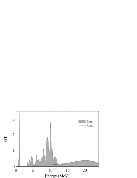
FIG. 3.: Experimental GT$-$ strength in ⁵⁴Fe [4]

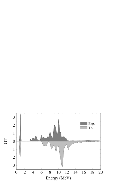
FIG. 4.: Experimental GT$-$ strength in ⁵⁴Fe after QFS subtraction [4], compared to $t=3\rightarrow t=4$ calculations.

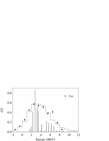
FIG. 5.: Experimental GT+ strength in ⁵⁴Fe [2],compared to $t=3\rightarrow t=3$ calculations.

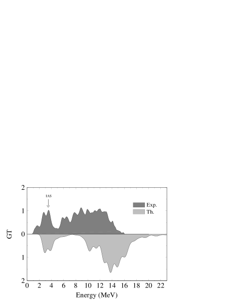
FIG. 6.: Experimental GT$-$ strength in ⁵⁶Fe [3],compared to $t=2\rightarrow t=4$ calculations. The IAS peak has not been removed from the data, but it is not included in the calculations.

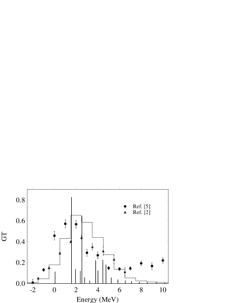
FIG. 7.: Experimental GT+ strength in ⁵⁶Fe [2, 5],compared to $t=2\rightarrow t=2$ calculations.

REFERENCES

- [1] M.C. Vetterly et al., Phys. Rev. C 40, 559 (1989).
- [2] T. Rönnqvist et al., Nucl. Phys. A563, 225 (1993).
- [3] J. Rapaport et al., Nucl. Phys. A410, 371 (1983).
- [4] B. D. Anderson, C. Lebo, A. R. Baldwin, T. Chittrakarn, R. Madey, and J. W. Watson, Phys. Rev. C 41, 1474 (1990).
- [5] S. El-Kateb et al., Phys. Rev. C 49, 3120 (1994).
- [6] G. M. Fuller, W. A. Fowler and M. J. Newman, Astophys. J. 252, 715 (1982)
- [7] S.D. Bloom and G.M. Fuller, Nucl. Phys. A440, 511 (1985).
- [8] F. Petrovich, H. Mc Manus, V. A. Madsen and J. Atkinson, Phys. Rev. Lett. 22, 895 (1969).
- [9] M. B. Aufderheide, S. D. Bloom, D. A. Resler, G. J. Mathews, Phys. Rev. C 48, 1677 (1993).
- [10] J. F. A. van Hienen, W. Chung and B. H. Wildenthal, Nucl. Phys. A269, 159 (1976).
- [11] J. E. Koops and P. W. M. Glaudemans, Z. Phys. A280, 181 (1977).
- [12] K. Muto, Nucl. Phys. A451, 481 (1986).
- [13] A. Yokoyama and H. Horie, Phys. Rev. C 31,1012 (1985).
- [14] N. Auerbach, G. F. Bertsch, B. A. Brown and L. Zhao, Nucl. Phys. A556, 190 (1993).
- [15] W. A. Richter, M. G. van der Merwe, R. E. Julies and B. A. Brown, Nucl. Phys. A523, 325 (1990).
- [16] J. Engel, P. Vogel and M. R. Zirnbauer, Phys. Rev. C 37, 731 (1988).
- [17] Y. Alhassid, D. J. Dean, S. E. Koonin, G. Lang and W. E. Ormand, Phys. Rev. Lett. 72, 613 (1994).
- [18] E. Caurier, A. P. Zuker, A. Poves and G. Martínez-Pinedo, Phys. Rev. C 50, 225 (1994).
- [19] T.T.S. Kuo and G.E. Brown, Nucl. Phys. A114, 241 (1968).
- [20] A. Poves and A. Zuker, Phys. Rep. 70, 235 (1981).
- [21] E. Caurier, code ANTOINE, Strasbourg 1989.
- [22] N. Anantaraman et al., Phys. Rev. C 44, 398 (1991).
- [23] D. J. Dean, P. B. Radha, K. Langanke, Y. Alhassid, S. E. Koonin and W. E. Ormand, Phys. Rev. Lett. 72, 4066 (1994).
- [24] B. A. Brown and B. H. Wildenthal, At. Data Nucl. Data Tables 33, 347 (1985).
- [25] F. Osterfeld, Rev. Mod. Phys. 64, 491 (1992).
- [26] E. Caurier, A. Poves and A. P. Zuker, Phys. Rev. Lett. 74 1517 (1995).
- [27] D. J. Dean, private communication.
- [28] K. Langanke et al., Caltech preprint, march 1995. NUC-TH/9504019