Instant Two-Body Equation in Breit Frame

Abstract

A quasipotential formalism for elastic scattering from relativistic bound states is based on applying an instant constraint to both initial and final states in the Breit frame. This formalism is advantageous for the analysis of electromagnetic interactions because current conservation and four momentum conservation are realized within a three-dimensional formalism.[1] Wave functions are required in a frame where the total momentum is nonzero, which means that the usual partial wave analysis is inapplicable. In this work, the three-dimensional equation is solved numerically, taking into account the relevant symmetries. A dynamical boost of the interaction also is needed for the instant formalism, which in general requires that the boosted interaction be defined as the solution of a four-dimensional equation. For the case of a scalar separable interaction, this equation is solved and the Lorentz invariance of the three-dimensional formulation using the boosted interaction is verified. For more realistic interactions, a simple approximation is used to characterize the boost of the interaction.

I INTRODUCTION

The theory of relativistic bound states in quantum field theory features four-dimensional equations and, in principle, an infinite number of degrees of freedom. Practical methods to solve the problem are not available and it is therefore common to reduce its complexity. In this paper, we discuss a covariant reduction to three dimensions and a finite number of degrees of freedom.[1] The interactions used are instantaneous. The formalism is tractable and it is applied to the deuteron bound state problem.

A general technique for reducing four-dimensional dynamics to three dimensions is to introduce a constraint which fixes one component of a four-vector in terms of the others.[2] This may be done covariantly, but the resulting formalism may possess unphysical asymmetries or singularities. An example is when one particle is constrained to its mass shell, and a second, identical particle is not.[3] Symmetry with respect to exchange of particle labels is lost. It is possible to respect the Pauli Principle by use of appropriately defined interactions, but they are cumbersome and they possess unphysical singularities which must be removed by hand. [4]

Symmetrical three-dimensional reductions have been used recently by Tjon and collaborators.[5, 6] Our work is similar but is based on the three-dimensional formalism developed by Mandelzweig and Wallace[7, 8], with an instant constraint at non-zero total momentum.[1] An instant constraint maintains symmetry with respect to exchange of particle labels and yields a constrained equation for relativistic bound states with no unphysical singularities. In this regard, it is an attractive alternative to reductions in which one particle is constrained to its mass shell. Although unphysical singularities are avoided, they are not entirely absent. They are expected to appear in corrections to the theory and in the four-dimensional equations for the boost of the interaction. Unphysical singularities are an unsolved problem for quasipotential approaches. In our approach to elastic electron scattering from a two-body bound state, they play no role.

A theory of bound states needs to be complemented by a corresponding theory of currents, e.g., the electromagnetic current. It is necessary to maintain a well-defined connection to quantum field theory and, for this reason, the Bethe-Salpeter formalism is the preferred starting point for the two-body problem. The associated currents have been formulated by Mandelstam in a celebrated paper.[9] In general, the currents depend on the interactions used to describe the bound state and a consistent relationship between the two is mandatory in order to conserve the electromagnetic current. An attractive feature of the instant formalism we discuss is that a Ward-Takahashi identity is realized at the level of the relativistic impulse approximation, thus guaranteeing current conservation for elastic matrix elements. There is a price associated with the current conservation. In the analysis of elastic electromagnetic scattering, a boost of the interaction is necessary in order to calculate the bound state wave functions in the Breit frame, where the total three-momentum is nonzero.

Dirac showed that the boost operator must depend on the interactions when the generators of the Poincare group are quantized at an instant of time.[10] This has its counterpart in the instant quasipotential formalism. A dynamical, four-dimensional equation must be solved to determine the instant quasipotential corresponding to different values of the total three-momentum. We distinguish between a kinematical boost and a dynamical one. The former is simpler because it is effected in the same fashion as for free particles and this is an advantage of a covariant formalism.[3, 4]. The latter is required in an instant formalism. In the work of Hummel and Tjon,[6] an instant quasipotential is used together with a kinematical boost. This leads to an inconsistency with respect to current conservation in matrix elements. In the present work, we develop methods to handle the dynamical boost that are consistent with current conservation for electromagnetic interactions.

For the special case of a scalar, separable interaction, the dynamical equation corresponding to a boost of the interaction is solved exactly and we verify that the mass of the deuteron is invariant when it is used. The boosted interaction varies rather slowly with the momentum for the deuteron and it may be approximated by a renormalization of the strength of the rest-frame interaction. This approximation is used in our analysis of electromagnetic form factors, which will be the subject of another paper.

This work contains the analysis and methods of solution for wave functions in the Breit frame. Because the total three-momentum is nonzero, the usual partial wave analysis is inapplicable. The wave functions are obtained by solving the three-dimensional integral equations using appropriately boosted interactions. Section II reviews the quasipotential equations in a frame where total three-momentum is nonzero. Section III discusses the equation which relates the quasipotential in different frames and presents the solution for a scalar, separable interaction. In Section IV, we discuss the symmetries of the relativistic bound state equations and use them to reduce the equations to a solvable form for the case of a boson-exchange interaction. Section V presents results for the deuteron wave functions and their variation with the total momentum of the bound state. Section VI presents some concluding remarks.

II Relativistic bound-state equation

The two-body equation with instant constraint has been derived in Ref. [7] in the rest frame of the two-body system. The derivation incorporates crossed graphs using a form of the eikonal approximation. The same derivation carried out in a frame where the total momentum is nonzero yields the three-dimensional quasipotential equation,

$$\psi({\bf p};P)=g_{0}({\bf p};P)\int\!\!\frac{d^{3}k}{(2\pi)^{3}}\hat{V}({\bf p},{\bf k};P)\psi({\bf k};P),$$ (1)

with relative and total momenta $p\equiv(p_{1}-p_{2})/2$ and $P\equiv p_{1}+p_{2}$ ($p^{0}=0,{\bf{P}}\equiv P^{z}\hat{\bf z}$). The three-dimensional propagator is expressed in terms of projection operators for positive- and negative-energy states as follows,

$$g_{0}({\bf p},P)=\sum_{\rho_{1},\rho_{2}}\frac{\Lambda_{1}^{\rho_{1}}({\bf p}_{1})\Lambda_{2}^{\rho_{2}}({\bf p}_{2})}{(\rho_{1}+\rho_{2})(E_{P}/2)-\epsilon_{1}-\epsilon_{2}},$$ (2)

where $\rho_{i}=\pm$, $\Lambda_{i}^{\rho_{i}}({\bf p}_{i})=\rho_{i}P_{i}^{\rho_{i}}\gamma^{0}_{i}$, where $P_{i}^{\rho_{i}}\equiv u^{\rho_{i}}_{i}(\rho_{i}{\bf p}_{i})[u^{\rho_{i}}_{i}(\rho_{i}{\bf p}_{i})]^{\dagger}$ are projection operators obeying $P_{i}^{\rho_{i}}P_{i}^{\rho^{\prime}_{i}}=\delta_{\rho_{i},\rho^{\prime}_{i}}.$ Dirac spinors used obey the hermitian normalization condition (A3). Moreover, $\epsilon_{i}\equiv\sqrt{m^{2}+{\bf p}^{2}_{i}}$ (${\bf p}_{1,2}={1\over 2}{\bf P}\pm{\bf p}$) and $P^{0}=E_{P}\equiv\sqrt{M^{2}+{\bf P}^{2}}$ are on-shell energies, and nucleon and deuteron masses are $m$ and $M$. This propagator differs from the Dirac two-body propagator of Refs. [7] only by use of the instant constraint in the frame where the two-body system moves with momentum ${\bf P}$, instead of in the rest frame.

As discussed in Ref. [8], it is possible to use the constraint $P\cdot p=0$ to develop a covariant formalism corresponding to instant interactions in the rest frame. If this is done, solutions of the equation can be boosted kinematically on a 3D surface embedded in the 4D space and defined by the constraint $p\cdot P=0$. However, this constraint is not compatible with the momentum transfer $q$ in interactions. If in the initial state the constraint $P\cdot p=0$ is satisfied, the corresponding constraint for the final state, namely $(P+q)\cdot(p\pm{1\over 2}q)=0$, depending on which particle absorbs the momentum transfer, cannot be satisfied. Absorption of the momentum transfer requires that the wave function be known off the 3D surface defined by the constraint. In contrast, a compatible formalism can be obtained by adopting the constraint $p^{0}=0$ in the Breit frame in place of the covariant one. The Breit frame corresponds to initial momentum $P_{i}=(E_{P},0,0,-{1\over 2}q)$ and final momentum $P_{f}=(E_{P},0,0,{1\over 2}q)$, where $E_{P}=\sqrt{M^{2}+q^{2}/4}$. It has the special property that $q^{0}=0$ for elastic interactions and thus is consistent with conservation of the four-momentum and three-dimensional wave functions.

The inverse propagator is easily obtained from the projection property and it is,

$$g^{-1}_{0}({\bf p};P)=\gamma^{0}_{1}\gamma^{0}_{2}\left[(E_{P}/2-\hat{\rho}_{1}\epsilon_{1})\hat{\rho}_{2}+(E_{P}/2-\hat{\rho}_{2}\epsilon_{2})\hat{\rho}_{1}\right],$$ (3)

with $\hat{\rho}_{i}=h({\bf p}_{i})/\epsilon_{i}$ (thus $\hat{\rho}_{i}u^{\pm}_{i}({\pm\bf p}_{i})=\pm u^{\pm}_{i}({\pm\bf p}_{i})$). The normalization condition for the two-body wave function is,

$$1 = {1\over{2E_{P}}}\int\!\!\frac{d^{3}pd^{3}k}{(2\pi)^{6}}\overline{\psi}({\bf p};P)\left[\gamma^{0}_{1}\gamma^{0}_{2}\frac{\hat{\rho}_{1}+\hat{\rho}_{2}}{2}(2\pi)^{3}\delta({\bf p}-{\bf k})\right.\left.-\left(\frac{\partial}{\partial P^{0}}\hat{V}({\bf p},{\bf k},P)\right)\right]\psi({\bf k};P).$$ (4)

III Boost of the Quasipotential

In quasipotential approaches, the quasipotential kernel is formally related to the Bethe-Salpeter kernel by,

$$K^{QP}(P)=K^{BS}(P)+iK^{BS}(P)\Delta(P)K^{QP}(P),$$ (5)

where a four-dimensional integration is implied over relative momentum, $p$, and

$$\Delta(P)\equiv G^{BS}_{0}(P)-G^{QP}_{0}(P),$$ (6)

$$G^{BS}(P) = \frac{\bigl{[}p_{1}\cdot\gamma_{1}+m\bigr{]}}{\bigl{[}p_{1}^{2}-m^{2}+i\eta\bigr{]}}\,\frac{\bigl{[}p_{2}\cdot\gamma_{2}+m\bigr{]}}{\bigl{[}p_{2}^{2}-m^{2}+i\eta\bigr{]}},$$ (7)

and

$$G^{QP}_{0}(P)=-ig_{0}({\bf p},P)2\pi\delta(p^{0})$$ (8)

in our approach. The quasipotential $\hat{V}$ used in Eq. (1) corresponds to $K^{QP}$ with initial and final momenta restricted to the constraint space, i.e., $p_{0}=0$. As emphasized in the notation, the quasipotential depends in general on the total four-momentum, $P$. The quasipotential propagator involving $p^{0}=0$ corresponds to different constraints for different values of $P$. Only when the constraint is expressed covariantly does it have the same physical meaning at all $P$ values.

In order to obtain the quasipotential corresponding to an instant constraint at different four-momenta, one must in general solve Eq. (5) at each value of $P$. Alternatively, it is possible to eliminate the Bethe-Salpeter kernel to arrive at a direct relation of the quasipotential corresponding to two different momenta $P$ and $P_{0}$. We do this for a somewhat simplified case where the Bethe-Salpeter kernel is assumed not to depend on the total momentum, $P$, and find

$$K^{Q}(P) = K^{QP}(P_{0})+iK^{QP}(P_{0})\>[\Delta(P)-\Delta(P_{0})]\>K^{QP}(P).$$ (9)

In the present work, we consider the boost of the quasipotential from the rest frame, where momentum is $P_{0}=(M,{\bf 0})$, to a frame where the four momentum is $P=(E_{P},{\bf P})$.

The chief complication in solving for the quasipotential lies in the implied 4D integration. However, the problem is soluble for the case of a separable Bethe-Salpeter kernel of the form,

$$K=|\chi\rangle k\langle\chi|,$$ (10)

where $|\chi\rangle$ carries the dependence on relative momentum, $p$, and $k$ is a $16\times 16$ matrix. For the discussion of the separable potential case, we omit parts of the quasipotential propagator which arise from the treatment of crossed Feynman graphs because these contributions are not meaningful for a separable potential. A simpler quasipotential propagator is used which is expressible as,

$$G^{QP}=2\pi\delta(p^{0})\int\frac{dp^{0}}{2\pi}G^{BS},$$ (11)

which agrees with Eqs. (8) and (2) in the $+\,+$ and $-\,-$ rhospin states, but is zero in the $+\,-$ and $-\,+$ rhospin states.

It follows that the quasipotential also takes a separable form

$$K^{QP}(P)=|\chi\rangle k^{QP}(P)\langle\chi|.$$ (12)

where $k^{QP}(P)$ is also a $16\times 16$ matrix in the two-particle Dirac space. It is related to the Bethe-Salpeter kernel by the matrix equation,

$$k^{QP}(P)=k+k\overline{\Delta}(P)k^{QP}(P),$$ (13)

where

$$\overline{\Delta}(P)=i\int\frac{d^{4}p}{(2\pi)^{4}}\chi(p)^{2}\Delta(P)$$ (14)

is a $16\times 16$ matrix. Alternatively, one may relate the quasipotential matrices at two different momenta by use of Eq. (9), which leads to the matrix equation,

$$k^{QP}(P)=k^{QP}(P_{0})+k^{QP}(P_{0})[\overline{\Delta}(P)-\overline{\Delta}(P_{0})]k^{QP}(P).$$ (15)

Either Eq. (13) or (15) is readily solved, e.g., Eq. (13) yields

$$k^{QP}(P)=\bigl{\{}\openone-k\overline{\Delta}(P)]\bigr{\}}^{-1}k.$$ (16)

A Analysis for a scalar, separable potential

In order to gain insight into the nature of the boost of the quasipotential, we have solved for $k^{QP}(P)$ for the case of a deuteron bound by a scalar, separable interaction. This means that $k$ is a coupling constant, $g$, times the direct product of unit matrices in each particle’s Dirac space. Taking symmetries into account, we find

$$\overline{\Delta}(P) = \bigl{(}{1\over 2}P\cdot\gamma_{1}+m\bigr{)}\bigl{(}{1\over 2}P\cdot\gamma_{2}+m\bigr{)}\Delta_{1}(P)-\frac{P\cdot\gamma_{1}}{M}\frac{P\cdot\gamma_{2}}{M}\Delta_{2}(P)-\frac{\widetilde{P}\cdot\gamma_{1}}{M}\frac{\widetilde{P}\cdot\gamma_{2}}{M}\Delta_{3}(P)$$ (18)

$$-\biggl{(}\frac{P\cdot\gamma_{1}}{M}\frac{\widetilde{P}\cdot\gamma_{2}}{M}+\frac{\widetilde{P}\cdot\gamma_{1}}{M}\frac{P\cdot\gamma_{2}}{M}\biggr{)}\Delta_{4}(P)+\gamma_{1\perp}\cdot\gamma_{2\perp}\Delta_{5}(P),$$

where $P=(E_{P},0,0,P)$, $\widetilde{P}=(P,0,0,E_{P})$ and thus $P\cdot\widetilde{P}=0$. Vectors with the $\perp$ subscript have only x- and y-components and they are orthogonal to $P$ and $\widetilde{P}$. The quantities $\Delta_{n}(P)$ for n = 1 to 5 in this expression are determined by the following equations,

$$\Delta_{n}(P)=A^{BS}_{n}(P)-A^{QP}_{n}(P),$$ (19)

where

$$A^{BS}_{n}(P) = i\int\frac{d^{4}p}{(2\pi)^{4}}\left[\chi(p)\right]^{2}\bigl{[}p_{1}^{2}-m^{2}+i\eta\bigr{]}^{-1}\bigl{[}p_{2}^{2}-m^{2}+i\eta\bigr{]}^{-1}O_{n},$$ (20)

$$A^{QP}_{n}(P) = i\int\frac{d^{3}p}{(2\pi)^{3}}\left[\chi({\bf p})\right]^{2}\int\frac{dp^{0}}{2\pi}\bigl{[}p_{1}^{2}-m^{2}+i\eta\bigr{]}^{-1}\bigl{[}p_{2}^{2}-m^{2}+i\eta\bigr{]}^{-1}O_{n},$$ (21)

and

$$O_{1} = 1,$$ (22)

$$O_{2} = \biggl{(}\frac{p\cdot P}{M}\biggr{)}^{2},$$ (23)

$$O_{3} = \biggl{(}\frac{p\cdot\widetilde{P}}{M}\biggr{)}^{2},$$ (24)

$$O_{4} = \biggl{(}\frac{p\cdot P}{M}\frac{p\cdot\widetilde{P}}{M}\biggr{)},$$ (25)

$$O_{5} = p_{x}^{2}.$$ (26)

Symmetries in the Bethe-Salpeter case cause $A_{3}^{BS}=A_{5}^{BS}$, and $A_{4}^{BS}=0$.

It is convenient to take matrix elements of $\overline{\Delta}(P)$ between plane-wave Dirac spinors depending on the total momentum and defined as follows,

$$u^{+}({\bf{P}})=N_{P}\pmatrix{1\cr\frac{\textstyle{{\mathchoice{{\hbox{\boldmath$\displaystyle\sigma$}}}{{\hbox{\boldmath$\textstyle\sigma$}}}{{\hbox{\boldmath$\scriptstyle\sigma$}}}{{\hbox{\boldmath$\scriptscriptstyle\sigma$}}}}\cdot{\bf{P}}}}{\textstyle{E_{P}+M}}\cr},$$ (27)

$$u^{-}({\bf{P}})=N_{P}\pmatrix{\frac{{\textstyle{\mathchoice{{\hbox{\boldmath$\displaystyle\sigma$}}}{{\hbox{\boldmath$\textstyle\sigma$}}}{{\hbox{\boldmath$\scriptstyle\sigma$}}}{{\hbox{\boldmath$\scriptscriptstyle\sigma$}}}}\cdot{\bf{P}}}}{\textstyle{E_{P}+M}}\cr 1\cr}.$$ (28)

These states are eigenfunctions of $\gamma\cdot P/M=\pm 1$ and the normalization factor is

$$N_{P}\equiv\sqrt{\frac{E_{P}+M}{2M}},$$ (29)

where $E_{P}=\sqrt{P^{2}+M^{2}}$. Negative energy states have negative norm: $\bar{u}^{-}(P)u^{-}(P)=-1$. The matrix form of $\overline{\Delta}(P)$ is,

$$[\overline{\Delta}(P)]=\pmatrix{\overline{\Delta}^{\,++,++}(P)&\overline{\Delta}_{\sigma}(P)&\sigma_{2z}\Delta_{4}(P)&\sigma_{1z}\Delta_{4}(P)\cr\overline{\Delta}_{\sigma}(P)&\overline{\Delta}^{\,--,--}(P)&\sigma_{1z}\Delta_{4}(P)&\sigma_{2z}\Delta_{4}(P)\cr\sigma_{2z}\Delta_{4}(P)&\sigma_{1z}\Delta_{4}(P)&\overline{\Delta}^{\,+-,+-}(P)&\overline{\Delta}_{\sigma}(P)\cr\sigma_{1z}\Delta_{4}(P)&\sigma_{2z}\Delta_{4}(P)&\overline{\Delta}_{\sigma}(P)&\overline{\Delta}^{\,-+,-+}(P)\cr},$$ (30)

where

$$\overline{\Delta}^{\,++,++}(P) = \overline{u^{+}_{1}}({\bf P})\overline{u^{+}_{2}}({\bf P})\overline{\Delta}(P)u^{+}_{1}({\bf P})u^{+}_{2}({\bf P})=({1\over 2}M+m)^{2}\Delta_{1}(P)-\Delta_{2}(P),$$ (31)

$$\overline{\Delta}^{\,--,--}(P) = \overline{u^{-}_{1}}({\bf P})\overline{u^{-}_{2}}({\bf P})\overline{\Delta}(P)u^{-}_{1}({\bf P})u^{-}_{2}({\bf P})=({1\over 2}M-m)^{2}\Delta_{1}(P)-\Delta_{2}(P),$$ (32)

$$\overline{\Delta}^{\,+-,+-}(P) = \overline{u^{+}_{1}}({\bf P})\overline{u^{-}_{2}}({\bf P})\overline{\Delta}(P)u^{+}_{1}({\bf P})u^{-}_{2}({\bf P})=({1\over 4}M^{2}-m^{2})\Delta_{1}(P)-\Delta_{2}(P),$$ (33)

$$\overline{\Delta}^{\,-+,-+}(P) = \overline{u^{-}_{1}}({\bf P})\overline{u^{+}_{2}}({\bf P})\overline{\Delta}(P)u^{-}_{1}({\bf P})u^{+}_{2}({\bf P})=({1\over 4}M^{2}-m^{2})\Delta_{1}(P)-\Delta_{2}(P),$$ (34)

and

$$\overline{\Delta}_{\sigma}=-\sigma_{1z}\sigma_{2z}\Delta_{3}(P)+\mathchoice{{\hbox{\boldmath$\displaystyle\sigma$}}}{{\hbox{\boldmath$\textstyle\sigma$}}}{{\hbox{\boldmath$\scriptstyle\sigma$}}}{{\hbox{\boldmath$\scriptscriptstyle\sigma$}}}_{1\perp}\cdot\mathchoice{{\hbox{\boldmath$\displaystyle\sigma$}}}{{\hbox{\boldmath$\textstyle\sigma$}}}{{\hbox{\boldmath$\scriptstyle\sigma$}}}{{\hbox{\boldmath$\scriptscriptstyle\sigma$}}}_{2\perp}\Delta_{5}(P).$$ (35)

It follows that the solution of Eq. (16) may be found and thus the full structure of the quasipotential displayed: $k^{QP}=\{\openone-g\overline{\Delta}\}^{-1}g\openone$ leads to the matrix equation $[\openone-g\overline{\Delta}]\,[\openone]\,[k^{QP}]=g[\openone]$, thus,

$$[k^{QP}]=\bigl{(}\,g^{-1}\,[\openone]-[\openone]\,[\overline{\Delta}]\,[\openone]\,\bigr{)}^{-1}.$$ (36)

A subtlety here is that the matrix for the unit operator is $[\openone]=diag\{1,1,-1,-1\}$. It is straightforward to realize $k^{QP}$ numerically by calculating the inverse implied in Eq. (36).

In the case of a separable potential, one may readily solve the Bethe-Salpeter wave equation or the quasipotential wave equation, using kernels appropriate to each. For the Bethe-Salpeter equation, we find

$$\phi^{BS}(P)=i\langle\chi|G^{BS}(P)|\chi\rangle\cdot k\cdot\phi^{BS},$$ (37)

and for the quasipotential equation,

$$\phi^{QP}(P)=i\langle\chi|G^{QP}(P)|\chi\rangle\cdot k^{QP}(P)\cdot\phi^{QP}.$$ (38)

These are equivalent if $k^{QP}$ is obtained from Eq. (13). The quantity $i\langle\chi|G^{BS}(P)|\chi\rangle$ has the same form as $\overline{\Delta}(P)$ using the $A^{BS}_{n}$ in place of $\Delta_{n}(P)$. Similarly, $i\langle\chi|G^{QP}(P)|\chi\rangle$ has the same form using $A^{QP}_{n}$ in place of $\Delta_{n}(P)$.

Numerical calculations for the scalar separable potential have been performed based on using $\chi(p)=(1+p^{2}/\mu^{2})^{-2}$ with $\mu=$ 200 MeV for the separable potential. The coupling constant $g$ is determined by the condition that a bound state exists for $M$ equal to the deuteron mass in the Bethe-Salpeter equation. Solutions corresponding to differing values of ${\bf P}$ are obtained from both equations and they demonstrate that the deuteron mass is invariant when the boosted quasipotential is used in Eq. (38).

Owing to dominance of the $+\,+$ states in the case of weak binding, an approximate characterization of the boost of the quasipotential is possible. A significant part of the effect is to renormalize the positive-energy matrix element in comparison to its value in the rest frame. The ratio of matrix elements defined as in Eq. (31) and calculated in the rest and moving frames is,

$$\lambda({\bf P})=\frac{{1\over 4}Tr\left[k^{QP}(P_{0})\right]^{++,++}}{{1\over 4}Tr\left[k^{QP}(P)\right]^{++,++}},$$ (39)

where the trace is over spins. This ratio may be used to approximate the boost as a similar renormalization of all matrix elements,

$$k^{QP}(P)\approx k^{QP}(P_{0})/\lambda({\bf P}).$$ (40)

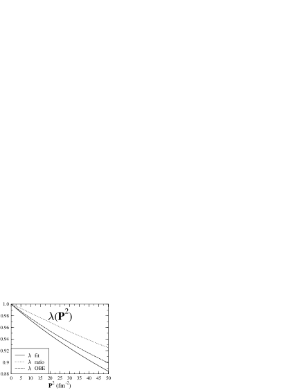
FIG. 1.: Renormalization factor of scalar quasipotential. Solid line shows $\lambda$ for invariant deuteron mass and dotted line shows prediction of Eq. (39). Dashed line shows result for a scalar, meson-exchange interaction.

A “fit” renormalization parameter can be determined as a function of ${\bf P}$ by using Eq. (40) and solving Eq. (38) for the value of $\lambda({\bf P})$ such that the mass is invariant. Figure 1 shows the variation of $\lambda({\bf P})$ with momentum for this fit case. For comparison, we show the “ratio” prediction based on Eq. (39), which is in reasonable agreement with the “fit” value. Also shown in Figure 1 is $\lambda({\bf P})$ fit to yield an invariant deuteron mass with the propagator of the next section, but using only the (scalar) $\sigma$ meson. The fit renormalization parameter $\lambda({\bf P})$ decreases for increasing ${\bf P}^{2}$ in a qualitatively similar fashion for scalar potentials of either the separable or one-boson-exchange type. Equation (36) would remain diagonal and proportional to $diag\{1,1,-1,-1\}$ if the Dirac structure remained scalar in the boost. As $|{\bf P}|$ increases, the matrix can be seen to change its structure. Owing to the dominance of the $++,++$ matrix elements, a significant part of the effect is a renormalization of the interaction.

If one has knowledge of the rest frame interaction $k^{QP}(P_{0})$, Eq. (15) may be used to determine $k^{QP}(P)$. This case is interesting because the NN interaction is usually regarded as known in the rest frame and the problem is to boost it to other frames. A more accurate approximation than a simple renormalization of all matrix elements is to expand perturbatively as follows,

$$k^{Q}(P)\approx k^{QP}(P_{0})+k^{QP}(P_{0})\left[\overline{\Delta}(P)-\overline{\Delta}(P_{0})\right]k^{QP}(P_{0}).$$ (41)

Keeping the second order term in Eq. (41) produces a form for $k^{QP}(P)$ that eliminates most of the momentum dependence of the mass. If a renormalization factor $\lambda({\bf P})$ is used with the approximation of Eq. (41), then a value $\lambda$ = 0.984 at ${\bf P}^{2}$ = 50 fm^-2 is required to keep the mass invariant, as compared with a value $\lambda$ = 0.882 when $k^{QP}(P)\approx k^{QP}(P_{0})/\lambda$ is used and $\lambda\equiv 1$ when the exact $k^{QP}(P)$ is used.

B Effective boost approximation

For the one-boson-exchange potential (in the rest frame) we use the Bonn potential (Bonn B, energy-independent, Thompson propagator)[11, 12]. This potential includes scalar, pseudo-vector, and vector meson exchanges ($\sigma,\delta,\eta,\pi,\omega,\rho$) and is detailed in Appendix B. When projected onto positive-energy plane-waves ($\rho_{1}\rho_{2}=++$) in the center-of-mass frame, the Dirac two-body $g_{0}$ of Eq. (2) reduces to the Thompson propagator and $V$ reduces to the Bonn potential. When negative-energies are included, there arise couplings in the quasipotential for which initial state rho spins of both particles are opposite to the final state rho spins. For example, $V^{++,--}$. An analysis of Feynman diagrams where such couplings arise shows that they generally are suppressed strongly in comparison with other couplings owing to the necessity of large time-like momentum transfer of order $2m$. For all other couplings, the instant constraint provides a reasonable starting approximation. To accommodate this fact, we eliminate the suppressed couplings by setting them to zero, i.e., $[\gamma^{0}_{1}\gamma^{0}_{2}V]^{\rho^{\prime}_{1},\rho^{\prime}_{2},\rho_{1},\rho_{2}}\to 0$ when $\rho^{\prime}_{1}=-\rho_{1}$ and $\rho^{\prime}_{2}=-\rho_{2}$.

To obtain the correct deuteron binding energy when negative energy sectors are included, we modify the Bonn B potential by increasing the scalar attraction about $6\%$, from $g^{2}_{\sigma}/4\pi=8.0769$ to $8.5503$. (See Table II.)

For the meson-exchange interaction, the simple approximation discussed above has been used to boost the quasipotential: $\hat{V}({\bf p}^{\prime}-{\bf p},{\bf P})=\hat{V}({\bf p}^{\prime}-{\bf p})/\lambda({\bf P})$, where $\lambda({\bf P})$ is fit to produce the correct deuteron total energy, $E_{P}=(M^{2}+{\bf P}^{2})^{1/2}$, using the two-body equation and propagator of Eqs. (1) and (2). This approximation can be shown to be consistent with current conservation when used in the analysis of elastic form factors. Note that the Dirac spinors appropriate to a moving deuteron are treated exactly and that the factor $\lambda({\bf P})$ approximates only the additional change of the potential required in an instant formalism. Figure 2 shows that the required change of the potential is modest, with $\lambda$ varying linearly vs. ${\bf P}^{2}$ over a wide range of values. For the full meson-exchange interaction, the renormalization factor $\lambda({\bf P}^{2})$ increases with ${\bf P}^{2}$, in contrast with the result of Figure 1 for a scalar interaction. This is caused by the differing boost factors required for different types of interaction. When $\lambda({\bf P})=1$ is used, the potential is too attractive and the binding energy of the deuteron increases from $2m-M\approx 2.2MeV$ at ${\bf P}^{2}=0$ to $2m-M\approx 4.2MeV$ at ${\bf P}^{2}=50fm^{-2}$. We have calculated the deuteron form factors based on $\lambda({\bf P})=1$ for comparison with those based on $\lambda({\bf P})$ determined so that $M$ is invariant. The differences are small.

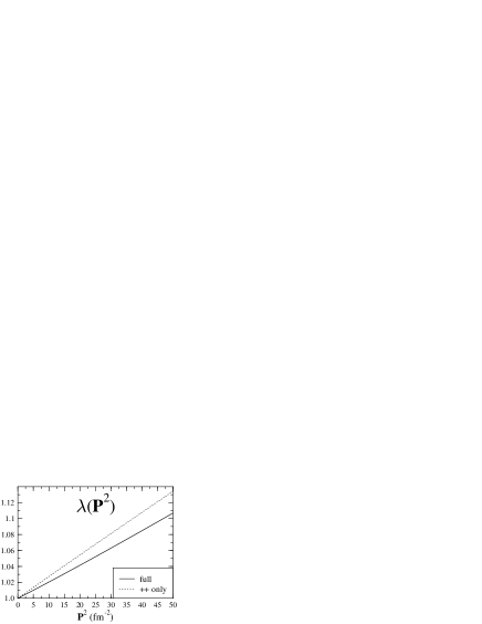
FIG. 2.: The scaling of the potential, $\hat{V}(p^{\prime}-p,{\bf P})=\hat{V}(p^{\prime}-p)/\lambda({\bf P}^{2})$, that produces constant deuteron mass, $M=(E_{P}^{2}-{\bf P}^{2})^{1/2}=2m-2.22464MeV$: full propagator (solid), $++$ states only (dotted).

IV Symmetries and reduction of the equation

The homogeneous equation is symmetric with respect to the operations of spatial reflection (${\cal P}$), particle exchange (${\cal P}_{\!\!12}$), and time-reversal (${\cal T}$), i.e., $g_{0}={\cal P}g_{0}{\cal P}^{-1}={\cal P}_{\!\!12}g_{0}{\cal P}_{\!\!12}^{-1}={\cal T}g_{0}{\cal T}^{-1}$, and $V$ is assumed to behave similarly. Thus it is possible to have solutions of the homogeneous equation with good corresponding parities:

$$\psi^{M}_{J}({\bf p},{\bf P}) = \eta{\cal P}\psi^{M}_{J}({\bf p},{\bf P}),$$ (42)

$$\psi^{M}_{J}({\bf p},{\bf P}) = \eta_{12}{\cal P}_{\!\!12}\psi^{M}_{J}({\bf p},{\bf P}),$$ (43)

$$\psi^{M}_{J}({\bf p},{\bf P}) = \eta_{T}(-1)^{M}{\cal T}\psi^{-M}_{J}({\bf p},{\bf P}),$$ (44)

where the parity, exchange parity, and anti-linear time-reversal operators are,

$${\cal P} = \gamma_{1}^{0}\gamma_{2}^{0}{\cal P}_{\!\!s},$$ (45)

$${\cal P}_{\!\!12} = {\cal P}_{\!\!ex}\Pi,$$ (46)

$${\cal T} = \sigma^{2}_{1}\sigma^{2}_{2}{\cal K},$$ (47)

where ${\cal K}$ is the operator of complex conjugation and ${\cal K}$ and ${\cal P}_{\!\!s}$ reverse three-momenta (${\cal P}_{\!\!s}{\bf p}=-{\bf p}$, ${\cal P}_{\!\!s}{\bf P}=-{\bf P}$); $\Pi$ reverses relative four-momentum ($\Pi p=-p$); and ${\cal P}_{\!\!ex}$ exchanges Dirac indices (${\cal P}_{\!\!ex}\gamma_{2}^{\mu}=\gamma_{1}^{\mu}{\cal P}_{\!\!ex}$, ${\cal P}_{\!\!ex}u^{\rho_{1}}_{1}(\rho_{1}{\bf p}_{1})=u^{\rho_{1}}_{2}(\rho_{1}{\bf p}_{1}){\cal P}_{\!\!ex}$, etc). For the deuteron $\eta=\eta_{12}=\eta_{T}=+1$. Note that ${\cal P}{\cal P}_{\!\!12}$ is equivalent to the H-parity operator of Kubis[13].

To find wave functions with good exchange parity, we rewrite the homogeneous equation using $\psi(-{\bf p},{\bf P})=\eta_{12}{\cal P}_{\!\!ex}\psi({\bf p},{\bf P})$ and find that,

$$\psi({\bf p}^{\prime};P) = g_{0}({\bf p}^{\prime};P)\gamma^{0}_{1}\gamma^{0}_{2}\int_{p_{z}>0}\!\frac{d^{3}p}{(2\pi)^{3}}\gamma^{0}_{1}\gamma^{0}_{2}\left[\hat{V}({\bf p}^{\prime},{\bf p};P)\right.+\left.\hat{V}({\bf p}^{\prime},-{\bf p};P)\eta_{12}{\cal P}_{\!\!ex}\right]\psi({\bf p};P).$$ (48)

Note that the necessary range of integration of $p_{z}$ is halved. To find wave functions with ${M}_{J}=0$ and good combined ${\cal P}{\cal T}$ parity, we will form eight basis functions with $+{\cal P}{\cal T}$ parity, and eight with $-{\cal P}{\cal T}$ parity.

The Breit frame total angular momentum operator is, ${\bf J}={\bf J}_{1}+{\bf J}_{2}=\vec{{\cal L}}+{\bf S}$, where $\vec{{\cal L}}={\bf l}+{\bf L}$, ${\bf l}={\bf r}\times{\bf p}$, ${\bf L}={\bf R}\times{\bf P}$, and ${\bf S}=\frac{1}{2}(\mathchoice{{\hbox{\boldmath$\displaystyle\sigma$}}}{{\hbox{\boldmath$\textstyle\sigma$}}}{{\hbox{\boldmath$\scriptstyle\sigma$}}}{{\hbox{\boldmath$\scriptscriptstyle\sigma$}}}_{1}+\mathchoice{{\hbox{\boldmath$\displaystyle\sigma$}}}{{\hbox{\boldmath$\textstyle\sigma$}}}{{\hbox{\boldmath$\scriptstyle\sigma$}}}{{\hbox{\boldmath$\scriptscriptstyle\sigma$}}}_{2})$. Because ${\bf J}^{2}$ and $J^{z}$ commute with $g^{-1}_{0}$ and $V$, solutions of the homogeneous equation are eigenfunctions of ${\bf J}^{2}$ and $J^{z}$. Also, wave functions with polarization states $M_{J}=\pm 1$ can be obtained from the $M_{J}=0$ state using raising and lowering operators, $\psi^{M_{J}\pm 1}=\sqrt{(J+M_{J})(J-M_{J}+1)}J^{\pm}\psi^{M_{J}}$. However, ${\bf l}$, ${\bf L}$, and ${\bf S}$ do not separately commute with $g^{-1}_{0}$, and the usual $LSJ$ partial-wave analysis is inapplicable. To proceed, we define cylindrical eigenfunctions of $J^{z}$ which form a basis for the $\phi$ dependence of the wave function:

$${\cal Y}^{M_{J}}_{s_{1},s_{2}}(\phi)=e^{i(M_{J}-s_{1}-s_{2})\phi}|s_{1}\rangle|s_{2}\rangle,$$ (49)

where ${\bf p}=(p^{xy}\cos(\phi),p^{xy}\cos(\phi),p^{z})$ is the relative three-momentum, $J^{z}{\cal Y}^{M_{J}}=M_{J}{\cal Y}^{M_{J}}$, and $s_{i}=\pm\frac{1}{2}$ are the $+\hat{z}$ components of spin (parallel to ${\bf P}=P^{z}\hat{z}$). A related set of eigenfunctions which we call the $PT$ basis is given by,

$${\cal Y}^{M_{J}}_{e1} \equiv \frac{1}{\sqrt{2}}({\cal Y}^{M_{J}}_{++}+{\cal Y}^{M_{J}}_{--}),$$ (50)

$${\cal Y}^{M_{J}}_{o1} \equiv \frac{1}{\sqrt{2}}({\cal Y}^{M_{J}}_{++}-{\cal Y}^{M_{J}}_{--}),$$ (51)

$${\cal Y}^{M_{J}}_{e0} \equiv \frac{1}{\sqrt{2}}({\cal Y}^{M_{J}}_{+-}+{\cal Y}^{M_{J}}_{-+}),$$ (52)

$${\cal Y}^{M_{J}}_{o0} \equiv \frac{1}{\sqrt{2}}({\cal Y}^{M_{J}}_{+-}-{\cal Y}^{M_{J}}_{-+}),$$ (53)

where the $\pm$ subscripts are shorthand for $\pm\frac{1}{2},\pm\frac{1}{2}$. It will be shown in Appendix A that these eigenfunctions have good ${\cal P}{\cal T}$ parity if $M_{J}=0$. Each set of eigenfunctions is orthonormal,

$$\int\frac{d\phi}{2\pi}\left[{\cal Y}_{a^{\prime}}(\phi)\right]^{\dagger}{\cal Y}_{a}(\phi)=\delta_{a^{\prime},a},$$ (54)

where $a\equiv(s_{1},s_{2},M_{J})$ (or $a\equiv(\alpha,M_{J})$ with $\alpha\in\{e1,o1,e0,o0\}$) and $a^{\prime}$ is similarly defined.

To form a complete set of two-particle basis functions, the angular eigenfunctions are combined with Dirac spinors obeying the hermitian normalization, $u^{\rho{\dagger}}(\rho{\bf p})u^{\rho^{\prime}}(\rho^{\prime}{\bf p})=\delta_{\rho\rho^{\prime}}$ (A3),

$$\chi^{\rho_{1},\rho_{2}}_{a}({\bf p},{\bf P})\equiv u^{\rho_{1}}_{1}(\rho_{1}{\bf p}_{1})u^{\rho_{2}}_{2}(\rho_{2}{\bf p}_{2}){\cal Y}_{a}(\phi).$$ (55)

Either set of sixteen basis functions is an orthonormal set,

$$\int\frac{d\phi}{2\pi}\left[\chi^{\rho^{\prime}_{1},\rho^{\prime}_{2}}_{a^{\prime}}({\bf p},{\bf P})\right]^{\dagger}\chi^{\rho_{1},\rho_{2}}_{a}({\bf p},{\bf P})=\delta_{\rho^{\prime}_{1},\rho_{1}}\delta_{\rho^{\prime}_{2},\rho_{2}}\delta_{a^{\prime},a},$$ (56)

and the wave functions are expanded in either set as follows,

$$\psi^{M}_{J}({\bf p};{\bf P})=\sum_{\rho_{1},\rho_{2},a}\chi^{\rho_{1},\rho_{2}}_{a}({\bf p},{\bf P})\psi^{\rho_{1},\rho_{2}}_{a}(p^{z},p^{xy};{\bf P}).$$ (57)

Using these plane-wave basis functions, the homogeneous equation (1 or 48) can be written in component form as

$$\psi^{\rho^{\prime}_{1},\rho^{\prime}_{2}}_{a^{\prime}}(p^{z},p^{xy};{\bf P})=\int\!\frac{k^{xy}dk^{xy}k^{z}}{(2\pi)^{2}}G^{\rho^{\prime}_{1},\rho^{\prime}_{2}}_{a^{\prime}}(p^{z},p^{xy};{\bf P})V^{\rho^{\prime}_{1},\rho^{\prime}_{2};\rho_{1},\rho_{2}}_{a^{\prime};a}(p^{z},p^{xy};k^{z},k^{xy})\psi^{\rho_{1},\rho_{2}}_{a}(k^{z},k^{xy};{\bf P})$$ (58)

or

$$\psi^{\rho^{\prime}_{1},\rho^{\prime}_{2}}_{a^{\prime}}(p^{z},p^{xy};{\bf P}) = \int_{k_{z}>0}\!\frac{k^{xy}dk^{xy}k^{z}}{(2\pi)^{2}}G^{\rho^{\prime}_{1},\rho^{\prime}_{2}}_{a^{\prime}}(p^{z},p^{xy};{\bf P})$$ (61)

$$\hskip 18.06749pt\times V^{\rho^{\prime}_{1},\rho^{\prime}_{2};\rho_{1},\rho_{2}}_{(k_{z}>0)\;a^{\prime};a}(p^{z},p^{xy};k^{z},k^{xy})\psi^{\rho_{1},\rho_{2}}_{a}(k^{z},k^{xy};{\bf P}),$$

where the diagonal hermitian propagator is

$$\int\frac{d\phi}{2\pi}\left[\chi^{\rho^{\prime}_{1},\rho^{\prime}_{2}}_{a^{\prime}}({\bf p},{\bf P})\right]^{\dagger}g_{0}({\bf p};{\bf P})\gamma^{0}_{1}\gamma^{0}_{2}\left[\chi^{\rho_{1},\rho_{2}}_{a}({\bf p},{\bf P})\right]=G^{\rho^{\prime}_{1},\rho^{\prime}_{2}}(p^{z},p^{xy};{\bf P})\delta_{\rho^{\prime}_{1},\rho_{1}}\delta_{\rho^{\prime}_{2},\rho_{2}}\delta_{a^{\prime},a},$$ (62)

with

$$G^{\rho^{\prime}_{1},\rho^{\prime}_{2}}(p^{z},p^{xy};{\bf P}) \equiv \left[(\rho^{\prime}_{1}+\rho^{\prime}_{2})\frac{E_{P}}{2}-\rho^{\prime}_{1}\rho^{\prime}_{2}(\epsilon_{1}+\epsilon_{2})\right]^{-1},$$ (63)

and the hermitian potential operator is given by,

$$V^{\rho^{\prime}_{1},\rho^{\prime}_{2};\rho_{1},\rho_{2}}_{a^{\prime};a}(p^{z},p^{xy};k^{z},k^{xy})\equiv\int\frac{d\phi_{p}d\phi_{k}}{(2\pi)^{2}}\left[\chi^{\rho^{\prime}_{1},\rho^{\prime}_{2}}_{a^{\prime}}({\bf p},{\bf P})\right]^{\dagger}\!\!\gamma^{0}_{1}\gamma^{0}_{2}\hat{V}({\bf p},{\bf k};P)\chi^{\rho_{1},\rho_{2}}_{a}({\bf k},{\bf P})$$ (64)

or

$$V^{\rho^{\prime}_{1},\rho^{\prime}_{2};\rho_{1},\rho_{2}}_{(k_{z}>0)\;a^{\prime};a}(p^{z},p^{xy};k^{z},k^{xy}) \equiv \int\frac{d\phi_{p}d\phi_{k}}{(2\pi)^{2}}\left[\chi^{\rho^{\prime}_{1},\rho^{\prime}_{2}}_{a^{\prime}}({\bf p},{\bf P})\right]^{\dagger}$$ (66)

$$\hskip 7.22743pt\times\gamma^{0}_{1}\gamma^{0}_{2}\left[\hat{V}({\bf p},{\bf k};P)+\hat{V}({\bf p},-{\bf k};P)\eta_{12}{\cal P}_{\!\!ex}\right]\chi^{\rho_{1},\rho_{2}}_{a}({\bf k},{\bf P}).$$

A detailed partial-wave analysis of the potential is contained in appendix B. Equation (58) or (61) is solved for $M_{J}=0$ at fixed values of total momentum using the Malfliet-Tjon iteration procedure[14] and numerical integration over $p^{xy}$ and $p^{z}$ (or radial and polar angle components). Wave functions with polarization states $M_{J}=\pm 1$ are obtained from the $M_{J}=0$ state by using the raising and lowering operator, $\psi^{M_{J}\pm 1}=\sqrt{(J+M_{J})(J-M_{J}+1)}J^{\pm}\psi^{M_{J}}$.

V Results for wave functions

Our wave functions vary as a function of both the magnitude and polar angle of relative momentum. To show how the wave functions change with total momentum, we project them onto standard LSJ basis functions and integrate out dependence on the polar angles,

$$\psi^{\rho_{1}\rho_{2}}_{lSJM_{J}}(|{\bf p}|,{\bf P})\equiv\int d\Omega_{p}\left[{\cal Y}_{lSJM_{J}}(\hat{p})\right]^{\dagger}\psi^{M_{J}}({\bf p},{\bf P}),$$ (67)

where the LSJ basis functions are given by,

$${\cal Y}^{M_{J}}_{lSJ}(\hat{\bf p})=\sum^{+1}_{m_{S}=-1} \langle l,S,m_{l},m_{S}|l,S,J,M_{J}\rangle Y_{l,m_{l}}(\theta,\phi)\>|S,m_{S}\rangle,$$ (68)

where $l$ and $S$ are the relative-orbital and spin angular momenta, ${\bf j}={\bf l}+{\bf S}$ and ${\bf l}={\bf r}\times{\bf p}$. These wave function components are shown in Fig. 3 for total momentum corresponding to ${\bf P}^{2}=$.0025, 12.5, 25 and 50$fm^{-2}$. A ‘probability’ for the wave function projections as defined by

$$P^{\rho_{1}\rho_{2}}_{lS}\equiv\frac{M}{E_{P}}\int p^{2}dp\left|\psi^{\rho_{1}\rho_{2}}_{lS}(|{\bf p}|,{\bf P})\right|^{2}$$ (69)

is shown in Table I based on the wave function normalization of Eq. (4).

	${\bf P}^{2}$
$\rho_{1}\rho_{2}lS$	0.0025$fm^{-2}$	12.5$fm^{-2}$	25$fm^{-2}$	50$fm^{-2}$
$++$01	0.9499	0.9433	0.9363	0.9226
$++$21	4.97$\times 10^{-2}$	5.59$\times 10^{-2}$	6.18$\times 10^{-2}$	7.22$\times 10^{-2}$
$+-$10	3.86$\times 10^{-5}$	4.00$\times 10^{-5}$	4.09$\times 10^{-5}$	4.18$\times 10^{-5}$
$+-$11	1.46$\times 10^{-4}$	1.19$\times 10^{-4}$	9.80$\times 10^{-5}$	6.86$\times 10^{-5}$
$--$01	2.70$\times 10^{-7}$	3.07$\times 10^{-7}$	3.20$\times 10^{-7}$	2.82$\times 10^{-7}$
$--$21	2.49$\times 10^{-6}$	1.72$\times 10^{-6}$	1.27$\times 10^{-6}$	8.01$\times 10^{-7}$
$P$(++)	0.99962	0.99921	0.99815	0.99475

TABLE I.: Wave function projection probabilities ($J=1$ and $M_{J}=0$). See text. $P(++)\equiv P($++$01)+P($++$21)$.

FIG. 3.: Dependence of Breit-frame wave functions on total momentum. In this figure $J=1$ and $M_{J}=0$, $P\approx 0MeV$(solid), $P=698MeV$(dotted), $P=987MeV$(dashed), and $P=1395MeV$(long dots).

VI Concluding remarks

The theory of relativistic bound states is formulated in three dimensions by use of an instant reduction of the Bethe-Salpeter formalism. This formalism is applicable to the analysis of elastic form factors and it is consistent with current conservation and four-momentum conservation. Elastic form factors involve matrix elements which are calculated in the Breit frame, thus requiring wave functions for the initial and final states that have been boosted to momentum ${\bf P}=\pm{1\over 2}{\bf q}$. These wave functions are calculated in this paper for the case of the deuteron. The form factors for the deuteron will be the subject of another paper.

The main issues addressed in this work are the boost of the interaction that is required and the solution of the quasipotential wave equation in frames where the total momentum is nonzero. We have shown that in general the boosted interaction is defined as the solution of a four-dimensional equation and that equation has been solved for the special case of a scalar, separable interaction. The main effect of the boost is to renormalize the dominant matrix elements of the interaction as three-momentum varies, although there is also in general a change in the Dirac structure of the interaction. An approximation which captures the renormalization effect is used for the more complicated one-boson exchange interaction. For momenta up to ${\bf P}^{2}$ = 50 fm^-2, the renormalization of the interaction is modest in the case of the deuteron, varying linearly with ${\bf P}^{2}$ and amounting to about a 10% reduction of the one-boson exchange potential at ${\bf P}^{2}$ = 50 fm^-2. A complete solution of the boost of the meson-exchange interaction is left as an unsolved problem. However, the separable potential analysis suggests that a perturbative expansion of Eq. (15) may provide accurate results for the boost.

The solutions for the quasipotential wave functions have been developed and the results show that there are modest variations as the deuteron is boosted to momenta up to ${\bf P}^{2}=$50 fm^-2, corresponding to ${\bf q}^{2}$ = 200 fm^-2. In a future article, they will be applied to the calculation of elastic form factors for the deuteron.

Support for this work by the U.S. Department of Energy under grants DE-FG02-93ER-40762 and DE-AC05-84ER40150 is gratefully acknowledged.

A Basis functions and operators

The hermitian plane-wave spinors for particle $i$ and denoted by $u_{i}^{\rho_{i}}(\rho_{i}{\bf k})$ are

$$u^{+}_{i}(+{\bf k}_{i})=N\left(\begin{array}[]{c}\mbox{1}\\ \frac{\textstyle\mathchoice{{\hbox{\boldmath$\displaystyle\sigma$}}}{{\hbox{\boldmath$\textstyle\sigma$}}}{{\hbox{\boldmath$\scriptstyle\sigma$}}}{{\hbox{\boldmath$\scriptscriptstyle\sigma$}}}_{i}\cdot{\bf k}_{i}}{\textstyle\epsilon_{i}+m}\end{array}\right),$$ (A3)

$$u^{-}_{i}(-{\bf k}_{i})=N\left(\begin{array}[]{c}\frac{\textstyle-\mathchoice{{\hbox{\boldmath$\displaystyle\sigma$}}}{{\hbox{\boldmath$\textstyle\sigma$}}}{{\hbox{\boldmath$\scriptstyle\sigma$}}}{{\hbox{\boldmath$\scriptscriptstyle\sigma$}}}_{i}\cdot{\bf k}_{i}}{\textstyle\epsilon_{i}+m}\\ \frac{\textstyle}{\textstyle}\mbox{1}\end{array}\right),$$ (A6)

with $N=\left(\frac{\epsilon_{i}+m}{2\epsilon_{i}}\right)^{1/2}$ and $\epsilon_{i}=\left(m^{2}+{\bf k}_{i}^{2}\right)^{1/2}$. It will be convenient later to use spinors with zero momentum which are related to the plane-wave spinors by,

$$u^{\rho_{i}}_{i}(\rho_{i}{\bf k}_{i})=N(1+\rho_{i}\frac{\mathchoice{{\hbox{\boldmath$\displaystyle\alpha_{i}$}}}{{\hbox{\boldmath$\textstyle\alpha_{i}$}}}{{\hbox{\boldmath$\scriptstyle\alpha_{i}$}}}{{\hbox{\boldmath$\scriptscriptstyle\alpha_{i}$}}}\cdot{\bf k}_{i}}{\epsilon_{i}+m})u^{\rho_{i}}_{i}({\bf 0}).$$ (A7)

Symmetry and Dirac operators acting on the basis functions will produce linear combinations (independent of $\phi$) of the basis functions. Some useful examples of this follow. The action of the operators on the Dirac and spin parts of the basis functions will be considered separately. Consider first the symmetry operators of Eqs. (45) – (47),

$${\cal P}u^{\rho_{i}}_{i}(\rho_{i}{\bf k}_{i}) = \rho_{i}u^{\rho_{i}}_{i}(\rho_{i}{\bf k}_{i}){\cal P}_{s},$$ (A8)

$${\cal P}_{12}u^{\rho_{i}}_{i}(\rho_{i}{\bf k}_{i}) = u^{\rho_{i}}_{j}(\rho_{i}{\bf k}_{j}){\cal P}_{12}\;(j\neq i),$$ (A9)

$${\cal T}u^{\rho_{i}}_{i}(\rho_{i}{\bf k}_{i}) = u^{\rho_{i}}_{i}(\rho_{i}{\bf k}_{i}){\cal T},$$ (A10)

and

$${\cal P}_{s}{\cal Y}^{M_{J}}_{s_{1},s_{2}}(\phi) = (-1)^{M_{J}-s_{1}-s_{2}}{\cal Y}^{M_{J}}_{s_{1},s_{2}}(\phi),$$ (A11)

$${\cal P}_{12}{\cal Y}^{M_{J}}_{s_{1},s_{2}}(\phi) = (-1)^{M_{J}-s_{1}-s_{2}}{\cal Y}^{M_{J}}_{s_{2},s_{1}}(\phi),$$ (A12)

$${\cal T}{\cal Y}^{M_{J}}_{s_{1},s_{2}}(\phi) = (-1)^{M_{J}}{\cal Y}^{-M_{J}}_{-s_{1},-s_{2}}(\phi).$$ (A13)

Similar relations for the ${\cal Y}^{M_{J}}_{\alpha}(\phi)$ of Eq. (50) $(\alpha\in\{e1,o1,e0,o0\})$ are easily derived from the above equations. In particular, for the basis $\chi^{\rho_{1},\rho_{2}}_{M_{J},\alpha}({\bf k},{\bf P})=u^{\rho_{1}}_{1}(\rho_{1}{\bf k}_{1})u^{\rho_{2}}_{2}(\rho_{2}{\bf k}_{2}){\cal Y}^{M_{J}}_{\alpha}(\phi)$,

$${\cal P}{\cal T}\chi^{\rho_{1},\rho_{2}}_{\alpha,M_{J}}({\bf k},{\bf P}) = \left\{\begin{array}[]{cc}+\rho_{1}\rho_{2}\chi^{\rho_{1},\rho_{2}}_{\alpha,-M_{J}}({\bf k},{\bf P})&\alpha=o1,e0\\ -\rho_{1}\rho_{2}\chi^{\rho_{1},\rho_{2}}_{\alpha,-M_{J}}({\bf k},{\bf P})&\alpha=e1,o0\\ \end{array}\right..$$ (A16)

Thus these basis functions have ${\cal P}{\cal T}=\pm 1$ if $M_{J}=0$. The condition ${\cal P}{\cal T}=\pm 1$ is equivalent to $Parity={\cal P}=\pm(-1)^{J+1}$ for the standard LSJ basis functions in the center-of-mass frame.

Consider next Dirac operators such as $\gamma^{0}_{i}$, $\gamma_{i}\cdot k_{i}$, $\gamma_{1}\cdot\gamma_{2}$, etc., acting on the simple basis functions given by $\chi^{\rho_{1},\rho_{2}}_{s_{1},s_{2}}({\bf k},{\bf P})=u^{\rho_{1}}_{1}({\bf 0})u^{\rho_{2}}_{2}({\bf 0}){\cal Y}^{M_{J}}_{s_{1},s_{2}}(\phi)$. Their effect on the zero-momentum spinors is particularly simple,

$$\gamma^{0}_{i}u^{\rho_{i}}_{i}({\bf 0}) = \rho_{i}u^{\rho_{i}}_{i}({\bf 0}),$$ (A18)

$$\gamma^{5}_{i}u^{\rho_{i}}_{i}({\bf 0}) = u^{-\rho_{i}}_{i}({\bf 0}).$$ (A19)

Moreover, spin operators acting on the basis functions produce linear combinations as follows,

$$\mathchoice{{\hbox{\boldmath$\displaystyle\sigma$}}}{{\hbox{\boldmath$\textstyle\sigma$}}}{{\hbox{\boldmath$\scriptstyle\sigma$}}}{{\hbox{\boldmath$\scriptscriptstyle\sigma$}}}_{1}\cdot\mathchoice{{\hbox{\boldmath$\displaystyle\sigma$}}}{{\hbox{\boldmath$\textstyle\sigma$}}}{{\hbox{\boldmath$\scriptstyle\sigma$}}}{{\hbox{\boldmath$\scriptscriptstyle\sigma$}}}_{2}{\cal Y}^{M}_{s_{1},s_{2}} = 4s_{1}s_{2}{\cal Y}^{M}_{s_{1},s_{2}}+2\delta_{s_{1},-s_{2}}{\cal Y}^{M}_{-s_{1},-s_{2}},$$ (A20)

$$\mathchoice{{\hbox{\boldmath$\displaystyle\sigma$}}}{{\hbox{\boldmath$\textstyle\sigma$}}}{{\hbox{\boldmath$\scriptstyle\sigma$}}}{{\hbox{\boldmath$\scriptscriptstyle\sigma$}}}_{1}\cdot{\bf k}_{1}{\cal Y}^{M}_{s_{1},s_{2}} = 2s_{1}k^{z}_{1}{\cal Y}^{M}_{s_{1},s_{2}}+k^{xy}_{1}{\cal Y}^{M}_{-s_{1},s_{2}},$$ (A21)

$$\mathchoice{{\hbox{\boldmath$\displaystyle\sigma$}}}{{\hbox{\boldmath$\textstyle\sigma$}}}{{\hbox{\boldmath$\scriptstyle\sigma$}}}{{\hbox{\boldmath$\scriptscriptstyle\sigma$}}}_{2}\cdot{\bf k}_{2}{\cal Y}^{M}_{s_{1},s_{2}} = 2s_{2}k^{z}_{2}{\cal Y}^{M}_{s_{1},s_{2}}+k^{xy}_{2}{\cal Y}^{M}_{s_{1},-s_{2}},$$ (A22)

where $k^{xy}_{1}=k^{xy}=-k^{xy}_{2}$. For the analysis of potential operators, it is useful to note,

$$\mathchoice{{\hbox{\boldmath$\displaystyle\sigma$}}}{{\hbox{\boldmath$\textstyle\sigma$}}}{{\hbox{\boldmath$\scriptstyle\sigma$}}}{{\hbox{\boldmath$\scriptscriptstyle\sigma$}}}_{1}\cdot{\bf q}_{1}{\cal Y}^{M}_{s_{1},s_{2}}(\phi_{k})=2s_{1}q^{z}_{1}{\cal Y}^{M}_{s_{1},s_{2}}(\phi_{k})+(p^{xy}_{1}e^{2s_{1}i\phi_{d}}-k^{xy}_{1}){\cal Y}^{M}_{-s_{1},s_{2}}(\phi_{k}),$$ (A23)

$$\mathchoice{{\hbox{\boldmath$\displaystyle\sigma$}}}{{\hbox{\boldmath$\textstyle\sigma$}}}{{\hbox{\boldmath$\scriptstyle\sigma$}}}{{\hbox{\boldmath$\scriptscriptstyle\sigma$}}}_{2}\cdot{\bf q}_{2}{\cal Y}^{M}_{s_{1},s_{2}}(\phi_{k})=2s_{2}q^{z}_{2}{\cal Y}^{M}_{s_{1},s_{2}}(\phi_{k})+(p^{xy}_{2}e^{2s_{2}i\phi_{d}}-k^{xy}_{2}){\cal Y}^{M}_{s_{1},-s_{2}}(\phi_{k}),$$ (A24)

where ${\bf q}_{i}\equiv{\bf p}_{i}-{\bf k}_{i}$ and $\phi_{d}\equiv\phi_{p}-\phi_{k}$.

Similar relations can be derived for the same Dirac operators acting on the sixteen $u^{\rho_{1}}_{1}({\bf 0})u^{\rho_{2}}_{2}({\bf 0}){\cal Y}^{M_{J}}_{\alpha}(\phi)$ basis functions. This can be accomplished by using the above equations and defining a basis transform between the two bases. Note that some of the above operators, such as $\gamma^{5}_{i}$, do not commute with ${\cal P}{\cal T}$.

B Partial-Wave Potential Analysis

In this appendix we sketch the partial wave analysis of the one-boson-exchange potential. This is most readily accomplished using the $\chi^{\rho_{1}\rho_{2}}_{s_{1},s_{2}}=u^{\rho_{1}}_{1}({\bf 0})u^{\rho_{2}}_{2}({\bf 0}){\cal Y}^{M_{J}}_{s_{1},s_{2}}(\phi)$ basis functions. The potential in this basis can easily be transformed to plane-wave or PT bases. The operator form of the potential is generated from the Feynman rules for meson propagators,

$$\Delta(q) = \frac{1}{q^{2}-\mu^{2}+i\eta},$$ (B1)

$$\Delta_{\alpha,\beta}(q) = \left[-g_{\alpha,\beta}+\frac{q_{\alpha}q_{\beta}}{\mu^{2}}\right]\Delta(q),$$ (B2)

and meson-nucleon vertices,

$$\Lambda_{S}(q) = -1,$$ (B3)

$$\Lambda_{P}(q) = i\gamma\cdot q\gamma^{5},$$ (B4)

$$\Lambda_{V}^{\alpha}(q) = (\gamma^{\alpha}+\frac{f}{2m}i\sigma^{\alpha,\nu}q_{\nu}),$$ (B5)

where the exchanged four momentum is $q=p_{1}-k_{1}=p-k=k_{2}-p_{2}$. The exchange of a single meson is given by $\Lambda(q)\Delta(q)\Lambda(-q)$ (or $\Lambda^{\alpha}(q)\Delta_{\alpha,\beta}(q)\Lambda^{\beta}(-q)$ for vector mesons) with a factor of $\tau_{1}\cdot\tau_{2}$ added to the exchange of isovector mesons and a coupling constant $g$ and form factor $F(q^{2})$ attached to each meson-nucleon vertex. Note that for the isoscalar deuteron, ${\bf\tau}_{1}\cdot{\bf\tau}_{2}\rightarrow-3$. The Bonn model form factors are,

$$F_{i}(q^{2}) = \frac{\Lambda^{2}_{i}-\mu^{2}_{i}}{\Lambda^{2}_{i}-q^{2}}.$$ (B6)

Thus the full one-boson-exchange potential is,

$$\hat{V}(p,k) = \sum_{i}g^{2}_{i}t_{i}\Delta_{i}(q)F^{2}_{i}(q^{2})\hat{V}_{i}(q),$$ (B7)

where $i$ is summed over the six mesons of Table II,

$$t_{i}\equiv\left\{\begin{array}[]{ccc}\tau_{1}\cdot\tau_{2}&if&i=isovector\;meson\\ 1&if&i=isoscalar\;meson\end{array}\right\},$$ (B8)

and

$$\hat{V}_{S}(q) \equiv \Lambda_{S}(q)\Lambda_{S}(-q),$$ (B9)

$$\hat{V}_{P}(q) \equiv -\Lambda_{P}(q)\Lambda_{P}(-q),$$ (B10)

$$\hat{V}_{V}(q) \equiv \Lambda^{\alpha}_{V}(q)\left[-g_{\alpha,\beta}+\frac{q_{\alpha}q_{\beta}}{\mu^{2}}\right]\Lambda^{\beta}_{V}(-q).$$ (B11)

Using Eqs. (A18) to (A24) it can be seen that

$$\gamma^{0}_{1}\gamma^{0}_{2}\hat{V}_{i}(q)\chi^{\rho_{1},\rho_{2}}_{s_{1},s_{2},M_{J}}({\bf k},{\bf P})=\chi^{\rho^{\prime\prime}_{1},\rho^{\prime\prime}_{2}}_{s^{\prime\prime}_{1},s^{\prime\prime}_{2},M_{J}}({\bf k},{\bf P})[V_{i}(p^{z},p^{xy},k^{z},k^{xy})]^{\rho^{\prime\prime}_{1},\rho^{\prime\prime}_{2},\rho_{1},\rho_{2}}_{s^{\prime\prime}_{1},s^{\prime\prime}_{2},s_{1},s_{2},M_{J};n}e^{in\phi_{d}},$$ (B12)

where $i=S,P,V$, $n=0,\pm 1,\pm 2$ and $\phi_{d}\equiv\phi_{p}-\phi_{k}$ with implicit sum over double prime variables. The exact form of $[V_{i}]$ is easily derived using a symbolic manipulation program such as Mathematica. For $\hat{V}_{V}$, note $\cos(\phi_{d})=(e^{i\phi_{d}}-e^{-i\phi_{d}})/2$. Next, the scalar part of the potential, which is a function of $\phi_{d}$ but not of $\phi_{p}$ or $\phi_{k}$ alone, can be integrated,

$$\int\frac{d\phi_{p}d\phi_{k}}{(2\pi)^{2}}\left[\chi^{\rho^{\prime}_{1},\rho^{\prime}_{2}}_{s^{\prime}_{1},s^{\prime}_{2},M^{\prime}_{J}}(\phi_{p})\right]^{\dagger}\Delta F^{2}e^{in\phi_{d}}\left[\chi^{\rho^{\prime\prime}_{1},\rho^{\prime\prime}_{2}}_{s^{\prime\prime}_{1},s^{\prime\prime}_{2},M_{J}}(\phi_{k})\right]=\delta_{\rho^{\prime}_{1},\rho^{\prime\prime}_{1}}\delta_{\rho^{\prime}_{2},\rho^{\prime\prime}_{2}}\delta_{s^{\prime}_{1},s^{\prime\prime}_{1}}\delta_{s^{\prime}_{2},s^{\prime\prime}_{2}}\delta_{M^{\prime}_{J},M_{J}}I_{F\Delta F}^{n-l},$$ (B13)

where $l\equiv M_{J}-s^{\prime}_{1}-s^{\prime}_{2}$ and

$$I_{F\Delta F}^{n}\equiv\int\frac{d\phi_{d}}{2\pi}\Delta(q)F^{2}(q^{2})e^{in\phi_{d}}.$$ (B15)

Bonn B potential parameters
(energy independent, Thompson propagator)
	$\pi$	$\eta$	$\rho$	$\omega$	$\delta$	$\sigma$
	PV-IV	PV-IS	V-IV	V-IS	S-IV	S-IS
$\mu$	.13803	.5488	.769	.7826	.983	.550
$\Lambda$	1.2	1.5	1.3	1.5	1.5	2.0
$g^{2}/4\pi$	14.6	5.0	.95	20.0	3.1155	8.0769
$f$			6.1	0
$g^{2}_{\sigma}/4\pi$ with negative energy sectors						8.5503

TABLE II.: Meson Parameters of the Bonn B model [12], and modification to $g^{2}_{\sigma}/4\pi$ when negative energy sectors are included. $M$ and $\Lambda$ in $GeV$. Nucleon mass is $m=.938926GeV$, deuteron binding energy is 2.224644MeV. Vector propagator is approximated by $\Delta_{\alpha,\beta}(q)\rightarrow-g_{\alpha,\beta}\Delta(q)$.

Combining the necessary factors, the partial-wave potential is,

$$[V(p^{z},p^{xy},k^{z},k^{xy})]^{\rho^{\prime}_{1},\rho^{\prime}_{2},\rho_{1},\rho_{2}}_{s^{\prime}_{1},s^{\prime}_{2},s_{1},s_{2},M_{J}}=\sum_{i}g^{2}_{i}t_{i}I_{F\Delta F}^{n-l}[V_{i}(p^{z},p^{xy},k^{z},k^{xy})]^{\rho^{\prime\prime}_{1},\rho^{\prime\prime}_{2},\rho_{1},\rho_{2}}_{s^{\prime\prime}_{1},s^{\prime\prime}_{2},s_{1},s_{2},M_{J};n}.$$ (B16)

This partial-wave potential based on zero-momentum spinors can be transformed to a plane-wave basis using the basis transform implied by Eqs. (A7), (A19), and (A21–A22),

Finally, the scalar $\phi_{d}$ integral of Eq. (B15) must be evaluated. This can be accomplished analytically using $z=e^{i\phi}$ and contour integration around the unit circle in the complex plane. We first express $\Delta F^{2}$ as a sum of simple denominators times $\phi_{d}$ independent coefficients using a partial fraction expansion. The integral of a simple meson denominator is given by,

$$I_{\mu}^{n} \equiv \int\frac{d\phi_{d}}{2\pi}\frac{e^{in\phi_{d}}}{a_{\mu}-b\cos(\phi_{d})}=-\int\frac{d\phi_{d}}{2\pi}\Delta(q)e^{in\phi_{d}}=\frac{z_{\mu}^{n}}{S_{\mu}},$$ (B17)

where $a_{\mu}\equiv\mu^{2}_{i}-(q(\phi_{d}=0))^{2}$, $b\equiv 2p_{xy}k_{xy}$ (thus $-\Delta^{-1}(q)=\mu^{2}-q^{2}=a_{\mu}-b\cos(\phi_{d})$), and $a_{\mu}>b$, $z_{\mu}\equiv(a-S)/b$, $S_{\mu}\equiv\sqrt{a^{2}-b^{2}}$. The denominators of the Bonn form factors, Eq. (B6), take the same form with $\mu$ replaced by $\Lambda$; thus $I_{\Lambda}\equiv I_{\mu}(\mu\rightarrow\Lambda)$. Using the partial fraction expansion for Bonn form factors and the simple integrals above,

$$I_{F\Delta F}^{n}=-I_{\mu}^{n}+I_{\Lambda}^{n}-(\Lambda^{2}-\mu^{2})\frac{\partial}{\partial a_{\Lambda}}I_{\Lambda}^{n}.$$ (B18)

This integral can be numerically checked using the following simple, well known, technique. We can write,

$$\Delta(q)F^{2}(q^{2}) = \Delta(q)+\left(F^{2}(\mu^{2})-F^{2}(q^{2})\right)\Delta(q),$$ (B19)

for any form factors with $F(\mu^{2})=1$. The first term is integrated using Eq. (B17), while the second term is evaluated numerically. Note the second term is non-singular even at $q^{2}=\mu^{2}$, which can not occur with instant constraints, but can occur if different constraints are used on the left and right of V.

REFERENCES

• [1] N. K. Devine and S. J. Wallace, Phys. Rev. C48, R973 (1993).
• [2] R. Blankenbecler and R. L. Sugar, Phys. Rev. 142, 1051 (1966); A. A. Logunov and A. N. Tavkhelidze, Nuovo Cimento 29, 380 (1963).
• [3] F. Gross, Phys. Rev. C 26, 2203 (1982).
• [4] F. Gross, J. W. Van Orden, and K. Holinde, Phys. Rev. C 45, 2094 (1992).
• [5] J. A. Tjon, in Hadronic Physics with Multi-GeV Electrons, edited by B. Desplanques and D. Goutte (Nova Science, Commack, New York, 1990).
• [6] E. Hummel and J. Tjon, Phys. Rev. Lett. 63, 1788 (1989) and Phys. Rev. C 42, 423 (1990) and Phys. Rev. C 49, 21 (1994).
• [7] V. B. Mandelzweig and S. J. Wallace, Phys. Lett. B197, 469 (1987).
• [8] S. J. Wallace and V.B. Mandelzweig, Nucl. Phys. A503, 673 (1989).
• [9] S. Mandelstam, Proc. R. Soc. London, Ser. A 233, 248 (1955).
• [10] P. A. M. Dirac, Rev. Mod. Phys. 21, 392 (1949).
• [11] N. K. Devine, Ph.D. thesis, University of Maryland, 1992.
• [12] R. Machleidt, Adv. in Nucl. Phys. (Plenum Press, New York, 1989), Vol. 19, edited by J. W. Negele.
• [13] J. J. Kubis, Phys. Rev. D 6, 547 (1972).
• [14] R. A. Malfliet and J. A. Tjon, Nucl. Phys. A127, 161 (1969).