Baryon Current Matrix Elements in a Light-Front Framework

Abstract

Current matrix elements and observables for electro- and photo-excitation of baryons from the nucleon are studied in a light-front framework. Relativistic effects are estimated by comparison to a nonrelativistic model, where we use simple basis states to represent the baryon wavefunctions. Sizeable relativistic effects are found for certain transitions, for example, to radial excitations such as that conventionally used to describe to the Roper resonance. A systematic study shows that the violation of rotational covariance of the baryon transition matrix elements stemming from the use of one-body currents is generally small.

1 Introduction

Much of what we know about excited baryon states has grown out of simple nonrelativistic quark models of their structure. These models were originally proposed to explain the systematics in the photocouplings of these states, which are extracted by partial-wave analysis of single-pion photoproduction experiments. This method can only give us information about baryon states which have already been produced in $\pi N$ elastic scattering, since a knowledge of the coupling constant for the outgoing $N\pi$ channel is necessary for the photocoupling extraction. Photoproduction experiments have also tended to have limited statistics relative to the $\pi N$ elastic scattering experiments.

The traditional theoretical approach is to describe the nucleon and its excitations using wavefunctions from nonrelativistic potential models, which describe baryons as being made up of ‘constituent’ quarks moving in a confining potential. This potential is provided by the interquark ‘glue’, which is taken to be in its adiabatic ground state. The quarks interact at short distance via one-gluon exchange. The electromagnetic current is also calculated using a simple nonrelativistic expansion of the single-quark transition operator, i.e., in the nonrelativistic impulse approximation. Not surprisingly, the resulting photocouplings and electroexcitation helicity amplitudes are frame dependent, with the problem becoming more severe when the photon transfers more momentum; current continuity is also violated. This is partly due to the nonrelativistic treatment, and partly due to the lack of two and three-body currents which must be present in this strongly-bound system.

Much more can be learned about these states from exclusive electroproduction experiments. The photocouplings are the values of transition form factors at the real-photon point $Q^{2}=0$ (here $Q^{2}=-q^{2}$, where $q^{\mu}$ is the four-momentum transferred from the electron); electroproduction experiments measure the $Q^{2}$ dependence of these form factors, and so simultaneously probe the spatial structure of the excited states and the initial nucleons. Both photoproduction and electroproduction experiments can be extended to examine final states other than $N\pi$, in order to find ‘missing’ states which are expected in symmetric quark models of baryons but which do not couple strongly to the $N\pi$ channel [1, 2]. Such experiments are currently being carried out at lower energies at MIT/Bates and Mainz. Many experiments to examine these processes up to higher energies and $Q^{2}$ values will take place at CEBAF.

The success of nonrelativistic quark models in describing the systematics of baryon photocouplings does not extend to the electroproduction amplitudes. The best measured of these amplitudes are those for elastic electron-nucleon scattering, the nucleon form factors. In a simple nonrelativistic model the charge radius of the proton is too small by a factor of almost two, and the form factors fall off too rapidly at larger $Q^{2}$ values. It has been suggested that the problem with the charge radius is due to the neglect of relativistic effects [3]. Similarly, the poor behavior at large $Q^{2}$ can be improved by going beyond the nonrelativistic approximation [4, 5, 6, 7] and by enlarging the limited (Gaussian) basis in which the wavefunctions are expanded [8]. Similar problems exist in the description of the $Q^{2}$ dependence of the transition form factors for the $\Delta{\textstyle{3\over 2}}^{+}(1232)$ resonance, which are also quite well measured. Although the experimental information about the transition form factors for higher mass resonances is limited [9], there are serious discrepancies between the predictions of the nonrelativistic model and the extracted amplitudes here also [10, 11, 12].

It is clear that, once the momentum transfer becomes greater than the mass of the constituent quarks, a relativistic treatment of the electromagnetic excitation is necessary. A consistent approach involves two main parts. First, the three-body relativistic bound-state problem is solved for the wavefunctions of baryons with the assumption of three interacting constituent quarks. Then these wavefunctions are used to calculate the matrix elements of one-, two- and three-body electromagnetic current operators. Results of model studies of the relativistic three-nucleon problem are available [13], and the problem of three constituent quarks in baryons is presently under investigation [14] (see also the comments in the final section). A useful first step is to consider transitions between substates in a general basis in which such wavefunctions may be expanded, such as a harmonic-oscillator basis. One can then examine successive approximations to the baryon wavefunctions with these un-mixed oscillator basis states as a starting point.

There are many competing approaches to the calculation of electromagnetic currents in relativistic bound states; we will use light-front relativistic Hamiltonian dynamics [15] here. The basis of this approach is to treat the constituents as particles rather than fields. It allows for an exact relativistic treatment of boosts, by removing the dependence on the interacting mass operator of the boost generators. As a consequence certain rotations become interaction dependent. Within this framework, one can set up a consistent impulse approximation, which minimizes the effects of many-body currents [15]. Current continuity can be enforced, though, as we shall see, not uniquely, and one can explicitly evaluate the degree to which the currents have the required rotational covariance properties [16].

Other authors have applied similar models to the study of these problems; Chung and Coester [4], Schlumpf [5], Weber [6], and Aznaurian [7] have studied nucleon elastic form factors in light-cone models with simple nucleon wavefunctions, and these models have been extended to the electroproduction amplitudes for the $\Delta(1232)$ resonance by Weber [17], in a model based on light-cone field theory, and by Aznaurian [7]. Bienkowska, Dziembowksi and Weber [18] have also applied a light-cone model to the study of the small electric-quadrupole $E2$ multipole in $\Delta{\textstyle{3\over 2}}^{+}(1232)$ electroproduction, and Weber [19] has also applied his model to the $S_{11}(1535)$ resonance.

Our goal is to examine the sensitivity of these photoproduction and electroproduction amplitudes to relativistic effects. Within the crude approximation of identifying un-mixed harmonic-oscillator wavefunctions with the states that they represent in zeroth order in the harmonic basis, we will examine the nucleon form factors, and the photo- and electroproduction amplitudes for the positive-parity states $\Delta{\textstyle{3\over 2}}^{+}(1232)$, the Roper resonance $N{\textstyle{1\over 2}}^{+}(1440)$, $N{\textstyle{1\over 2}}^{+}(1710)$, $\Delta{\textstyle{3\over 2}}^{+}(1600)$, and several negative-parity resonances including $N{\textstyle{1\over 2}}^{-}(1535)$ and $N{\textstyle{3\over 2}}^{-}(1520)$. We will show that relativistic effects are in general appreciable; the most striking relativistic effects we have seen are in the electroproduction amplitudes for radial excitations such as $N{\textstyle{1\over 2}}^{+}(1440)$ and $\Delta{\textstyle{3\over 2}}^{+}(1600)$. We also provide a systematic study of rotational covariance of the baryon transition matrix elements.

2 Conventions

Much of the light-front notation is presented in Ref. [15]. We present here the salient features needed to describe the calculation of current matrix elements.

2.1 Kinematics

A homogeneous Lorentz transformation $\Lambda$ describes the relation between between four-vectors, viz.,

$$p^{\mu}\to p^{\prime}{}^{\mu}=\Lambda^{\mu}{}_{\nu}p^{\nu}.$$ (1)

We also make use of the corresponding $SL(2,C)$ representation, denoted by ${\underline{\Lambda}}$. A rotationless boost is given by

$${\underline{L}}_{c}({\bf A})\equiv\exp[{\textstyle{1\over 2}}({\hat{\bf A}}\cdot{\mbox{\boldmath$\sigma$}})\sinh^{-1}|{\bf A}|].$$ (2)

Light-front kinematic variables are expressed in terms of four-vectors which are decomposed as $a^{\mu}=(a^{-},{\bf a}_{\perp},a^{+})$, where $a^{\pm}\equiv a^{0}\pm\hat{\bf n}\cdot{\bf a}$ and $\hat{\bf n}\cdot{\bf a}_{\perp}=0$. We adopt here the usual convention of setting $\hat{\bf n}$ parallel to the $z$ axis. It is also convenient to define a light-front vector

$${\tilde{\bf a}}\equiv({\bf a}_{\perp},a^{+}).$$ (3)

The $SL(2,C)$ representation of a light-front boost is

$${\underline{L}}_{f}({\tilde{\bf A}})\equiv\exp({\textstyle{1\over 2}}\sigma^{3}\ln A^{+})\exp[{\textstyle{1\over 2}}(A^{1}+iA^{2})(\sigma^{1}-i\sigma^{2})].$$ (4)

2.2 State Vectors

Free-particle state vectors $|{\tilde{\bf p}}\mu\rangle$ are labeled by the light-front vector ${\tilde{\bf p}}$ and satisfy the mass-shell condition

$$p^{-}=(m^{2}+{\bf p}_{\perp}^{2})/p^{+}.$$ (5)

They are normalized as follows:

$$\langle{\tilde{\bf p}}^{\prime}\mu^{\prime}|{\tilde{\bf p}}\mu\rangle=(2\pi)^{3}\delta_{\mu^{\prime}\mu}\delta({\tilde{\bf p}}^{\prime}-{\tilde{\bf p}})=(2\pi)^{3}\delta_{\mu^{\prime}\mu}\delta({\bf p}^{\prime}_{\perp}-{\bf p}_{\perp})\delta(p^{\prime}{}^{+}-p^{+}).$$ (6)

The state vectors introduced above employ light-front spin. Under a light-front boost, $p^{\prime}{}^{\mu}=\Lambda^{\mu}{}_{\nu}p^{\nu}$, the state vectors undergo the unitary transformation

$$U(\Lambda)|{\tilde{\bf p}}\mu\rangle=\sqrt{{p^{\prime}{}^{+}}\over p^{+}}|{\tilde{\bf p}}^{\prime}\mu\rangle,$$ (7)

with no accompanying Wigner rotation. These state vectors are related to this with ordinary (or canonical) spin via the relation the relation

$$|{\tilde{\bf p}}\mu\rangle=\sum_{\bar{\mu}}\sqrt{\omega_{m}({\bf p})\over p^{+}}|{\bf p}{\bar{\mu}}\rangle_{c}D^{({\textstyle{1\over 2}})}_{{\bar{\mu}}\mu}[{\underline{R}}_{cf}(p)],$$ (8)

where the Melosh rotation [20] is

$${\underline{R}}_{cf}(p)={\underline{L}}_{c}^{-1}({{\bf p}\over m}){\underline{L}}_{f}({{\bf p}\over m}).$$ (9)

2.3 Three-Body Kinematics

Consider three free particles with masses $m_{1}$, $m_{2}$ and $m_{3}$. We label their respective light-front momenta in an arbitrary frame by ${\tilde{\bf p}}_{1}$, ${\tilde{\bf p}}_{2}$ and ${\tilde{\bf p}}_{3}$. The total light-front momentum is

$${\tilde{\bf P}}={\tilde{\bf p}}_{1}+{\tilde{\bf p}}_{2}+{\tilde{\bf p}}_{3}.$$ (10)

Let ${\bf k}_{1}$, ${\bf k}_{2}$ and ${\bf k}_{3}$ be the ordinary three-momenta in a frame where the total momentum is zero:

$$\sum_{i=1}^{3}{\bf k}_{i}=0.$$ (11)

The two sets of momenta are related as follows:

$${\bf k}_{i\perp} ={\bf p}_{i\perp}-x_{i}{\bf P}_{\perp};\quad x_{i}=p_{i}^{+}/P^{+};$$

$$k_{i3} ={\textstyle{1\over 2}}\left[x_{i}M_{0}-{m_{i}^{2}+{\bf k}_{i\perp}^{2}\over x_{i}M_{0}}\right],$$ (12)

where $M_{0}$ is the invariant mass of the three-particle system:

$$M_{0} =\sum_{i=1}^{3}\omega_{m_{i}}({\bf k}_{i})=\sqrt{P^{+}P^{-}-{\bf P}_{\perp}^{2}}$$ (13)

$$=\left[\sum_{i=1}^{3}{m_{i}^{2}+{\bf k}_{i\perp}^{2}\over x_{i}}\right]^{\textstyle{1\over 2}},$$

where

$$\omega_{m}({\bf k})\equiv\sqrt{m^{2}+{\bf k}^{2}}.$$ (14)

The Jacobian of the transformation $({\tilde{\bf p}}_{1},{\tilde{\bf p}}_{2},{\tilde{\bf p}}_{3})\to({\tilde{\bf P}},{\bf k}_{1},{\bf k}_{2})$ is

$$\left|{\partial({\tilde{\bf p}}_{1},{\tilde{\bf p}}_{2},{\tilde{\bf p}}_{3})\over\partial({\tilde{\bf P}},{\bf k}_{1},{\bf k}_{2})}\right|={p_{1}^{+}p_{2}^{+}p_{3}^{+}M_{0}\over\omega_{m_{1}}({\bf k}_{1})\omega_{m_{2}}({\bf k}_{2})\omega_{m_{3}}({\bf k}_{3})P^{+}}.$$ (15)

3 Current Matrix Elements

To calculate the current matrix element between initial and final baryon states, we first expand in sets of free-particle states:

$$\langle M^{\prime}j;{\tilde{\bf P}}^{\prime}\mu^{\prime}|I^{+}(0)|Mj;{\tilde{\bf P}}\mu\rangle =(2\pi)^{-18}\int d{\tilde{\bf p}}_{1}^{\prime}\int d{\tilde{\bf p}}_{2}^{\prime}\int d{\tilde{\bf p}}_{3}^{\prime}\int d{\tilde{\bf p}}_{1}\int d{\tilde{\bf p}}_{2}\int d{\tilde{\bf p}}_{3}\sum$$ (16)

$$\quad\langle M^{\prime}j^{\prime};{\tilde{\bf P}}^{\prime}\mu^{\prime}|{\tilde{\bf p}}^{\prime}_{1}\mu^{\prime}_{1}{\tilde{\bf p}}^{\prime}_{2}\mu^{\prime}_{2}{\tilde{\bf p}}^{\prime}_{3}\mu^{\prime}_{3}\rangle$$

$$\quad\times\langle{\tilde{\bf p}}^{\prime}_{1}\mu^{\prime}_{1}{\tilde{\bf p}}^{\prime}_{2}\mu^{\prime}_{2}{\tilde{\bf p}}^{\prime}_{3}\mu^{\prime}_{3}|I^{+}(0)|{\tilde{\bf p}}_{1}\mu_{1}{\tilde{\bf p}}_{2}\mu_{2}{\tilde{\bf p}}_{3}\mu_{3}\rangle$$

$$\quad\times\langle{\tilde{\bf p}}_{1}\mu_{1}{\tilde{\bf p}}_{2}\mu_{2}{\tilde{\bf p}}_{3}\mu_{3}|Mj;{\tilde{\bf P}}\mu\rangle.$$

Here and henceforth, an empty summation sign denotes an implied sum over all repeated indices. We compute only the contributions from one-body matrix elements:

$$\langle{\tilde{\bf p}}^{\prime}_{1}\mu^{\prime}_{1}{\tilde{\bf p}}^{\prime}_{2}\mu^{\prime}_{2}{\tilde{\bf p}}^{\prime}_{3}\mu^{\prime}_{3}|I^{+}(0)|{\tilde{\bf p}}_{1}\mu_{1}{\tilde{\bf p}}_{2}\mu_{2}{\tilde{\bf p}}_{3}\mu_{3}\rangle$$

$$\qquad\approx\sum_{i=1}^{3}\langle{\tilde{\bf p}}_{i}^{\prime}\mu_{i}^{\prime}|I^{+}(0)|{\tilde{\bf p}}_{i}\mu_{i}\rangle\prod_{j\neq i}\left[\delta_{\mu_{j}^{\prime}\mu_{j}}(2\pi)^{3}\delta({\tilde{\bf p}}_{j}^{\prime}-{\tilde{\bf p}}_{j})\right].$$ (17)

The matrix elements for the struck quark are then written in terms of the Pauli and Dirac form factors for the constituent quarks

$$\langle{\tilde{\bf p}}^{\prime}\mu^{\prime}|I^{+}(0)|{\tilde{\bf p}}\mu\rangle=F_{1q}(Q^{2})\delta_{\mu^{\prime}\mu}-i(\sigma_{y})_{\mu^{\prime}\mu}{Q\over 2m_{i}}F_{2q}(Q^{2}).$$ (18)

Note that this implies that these current matrix elements depend only on $Q$ (${\bf q}$ is taken to lie along the x-axis) and not on the initial and final momentum of the struck quark, as in the nonrelativistic model.

The baryon state vectors are in turn related to wave functions as follows:

$$\langle{\tilde{\bf p}}_{1}\mu_{1}{\tilde{\bf p}}_{2}\mu_{2}{\tilde{\bf p}}_{3}\mu_{3}|Mj;{\tilde{\bf P}}\mu\rangle =\left|{\partial({\tilde{\bf p}}_{1},{\tilde{\bf p}}_{2},{\tilde{\bf p}}_{3})\over\partial({\tilde{\bf P}},{\bf k}_{1},{\bf k}_{2})}\right|^{-{1\over 2}}\langle{\textstyle{1\over 2}}{\bar{\mu}}_{1}{\textstyle{1\over 2}}{\bar{\mu}}_{2}|s_{12}\mu_{12}\rangle\langle s_{12}\mu_{12}{\textstyle{1\over 2}}{\bar{\mu}}_{3}|s\mu_{s}\rangle$$ (19)

$$\quad\times\langle l_{\rho}\mu_{\rho}l_{\lambda}\mu_{\lambda}|L\mu_{L}\rangle\langle L\mu_{L}s\mu_{s}|j\mu\rangle$$

$$\quad\times Y_{l_{\rho}\mu_{\rho}}({\hat{\bf k}}_{\rho})Y_{l_{\lambda}\mu_{\lambda}}({\hat{\bf K}}_{\lambda})\Phi(k_{\rho},K_{\lambda})$$

$$\quad\times D^{({\textstyle{1\over 2}}){{\dagger}}}_{{\bar{\mu}}_{1}\mu_{1}}[{\underline{R}}_{cf}({k}_{1})]D^{({\textstyle{1\over 2}}){{\dagger}}}_{{\bar{\mu}}_{2}\mu_{2}}[{\underline{R}}_{cf}({k}_{2})]$$

$$\quad\times D^{({\textstyle{1\over 2}}){{\dagger}}}_{{\bar{\mu}}_{3}\mu_{3}}[{\underline{R}}_{cf}({k}_{3})],$$

The quantum numbers of the state vectors correspond to irreducible representations of the permutation group. The spins $(s_{12},s)$ can have the values $(0,{\textstyle{1\over 2}})$, $(1,{\textstyle{1\over 2}})$ and $(1,{3\over 2})$, corresponding to quark-spin wavefunctions with mixed symmetry ($\chi^{\rho}$ and $\chi^{\lambda}$) and total symmetry ($\chi^{S}$), respectively [21]. The momenta

$${\bf k}_{\rho} \equiv{1\over\sqrt{2}}({\bf k}_{1}-{\bf k}_{2});$$

$${\bf K}_{\lambda} \equiv{1\over\sqrt{6}}({\bf k}_{1}+{\bf k}_{2}-2{\bf k}_{3})$$ (20)

preserve the appropriate symmetries under various exchanges of ${\bf k}_{1}$, ${\bf k}_{2}$ and ${\bf k}_{3}$. Note that ${\bf k}_{\rho}$ and ${\bf K}_{\lambda}$ as defined above also correspond to the nonrelativistic three-body Jacobi momenta. This is a definition of convenience, rather than a nonrelativistic approximation. The three momenta ${\bf k}_{i}$ are defined with relativistic kinematics, and the use of ${\bf k}_{\rho}$ and ${\bf K}_{\lambda}$ accounts for the fact that only two of the ${\bf k}_{i}$ are independent. It is also convenient for keeping track of the exchange symmetry of the three quarks. This definition allows use of the usual three-quark harmonic-oscillator wave functions as a basis, but there is nothing nonrelativistic about this choice.

4 Multipole Invariants

From the current operator $I^{\mu}(x)$, we define an auxiliary operator ${\hat{I}}^{s}_{\mu_{s}}(x)$, which has explicit components

$${\hat{I}}^{1}_{\pm 1}(x) =\mp{1\over\sqrt{2}}(I^{1}(x)\pm iI^{2}(x));$$

$${\hat{I}}^{1}_{0}(x) =I^{3}(x);$$

$${\hat{I}}^{0}_{0}(x) =I^{0}(x).$$ (21)

With these definitions, it was shown in Ref. [15] that the current matrix element between states with canonical spins and instant-form three-momenta could be written as follows:

$${}_{c}\langle M^{\prime}j^{\prime};{\bf P}^{\prime}\mu^{\prime}|{\hat{I}}^{s}_{\mu_{s}}(0)|Mj;{\bf P}\mu\rangle_{c}$$

$$\quad=\sqrt{M^{\prime}\over\omega_{M^{\prime}}({\bf P}^{\prime})}\sqrt{{\omega_{M}({\bf P}_{0})}\over{\omega_{M}({\bf P})}}(-1)^{s}{1\over\sqrt{2}}\sum\langle{\textstyle{1\over 2}}\alpha{\textstyle{1\over 2}}{\dot{\beta}}|s\mu_{s}\rangle\langle{\textstyle{1\over 2}}\zeta{\textstyle{1\over 2}}{\dot{\eta}}|{\bar{s}}{\bar{\mu}}_{s}\rangle$$

$$\quad\quad\times\langle l\mu_{l}{\bar{s}}{\bar{\mu}}_{s}|{\cal J}\mu_{\cal J}\rangle\langle j{\bar{\mu}}{\cal J}\mu_{\cal J}|j^{\prime}\mu^{\prime}\rangle$$

$$\quad\quad\times Y^{l}_{\mu_{l}}{}^{*}({\bf\hat{P}}_{0})[{\underline{L}}^{-1}_{c}({{\bf P}^{\prime}\over M^{\prime}})]_{\zeta\alpha}[{\underline{L}}_{c}({{\bf P}^{\prime}\over M^{\prime}})]^{{\dagger}}_{{\dot{\eta}}{\dot{\beta}}}D^{j{{\dagger}}}_{{\bar{\mu}}\mu}[{\underline{R}}_{c}({\underline{L}}_{c}({{\bf P}^{\prime}\over M^{\prime}}),P_{0})]\langle M^{\prime}j^{\prime}\parallel I_{l{\bar{s}}{\cal J}}(q^{2})\parallel Mj\rangle,$$ (22)

where

$$P_{0}=L_{c}^{-1}({{\bf P}^{\prime}\over M^{\prime}})P.$$ (23)

The Wigner rotation is

$${\underline{R}}_{c}({\underline{L}}_{c}({{\bf P}^{\prime}\over M^{\prime}}),P_{0})\equiv{\underline{L}}_{c}^{-1}({{\bf P}\over M}){\underline{L}}_{c}({{\bf P}^{\prime}\over M^{\prime}}){\underline{L}}_{c}({{\bf P}_{0}\over M})$$ (24)

All dynamical information is contained in the reduced matrix element $\langle M^{\prime}j^{\prime}\parallel I_{l{\bar{s}}{\cal J}}(q^{2})\parallel Mj\rangle$. The number of independent matrix elements is limited by the number of combinations of $l$, ${\bar{s}}$ and ${\cal J}$ which can couple together. Parity considerations provide the additional restriction:

$$\Pi^{\prime}\Pi(-1)^{l+{\bar{s}}}=+1.$$ (25)

where $\Pi^{\prime}$ and $\Pi$ are the intrinsic parities of the final and initial states, respectively. Time reversal provides another constraint for the case of elastic scattering. Finally, the continuity equation:

$$q_{\mu}\langle M^{\prime}P^{\prime}\mu^{\prime}|I^{\mu}(0)|MP\mu\rangle=0$$ (26)

further restricts the number of independent matrix elements.

The matrix element of $I^{+}(0)$ between light-front state vectors is

$$\langle M^{\prime}j^{\prime};{\bf P}^{\prime}\mu^{\prime}|I^{+}(0)|Mj;{\bf P}\mu\rangle$$

$$\quad=\sqrt{M^{\prime}\over P^{\prime}{}^{+}}\sqrt{{\omega_{M}({\bf P}_{0})}\over P^{+}}{1\over\sqrt{2}}\sum\left[-\langle{\textstyle{1\over 2}}\alpha{\textstyle{1\over 2}}{\dot{\beta}}|10\rangle+\langle{\textstyle{1\over 2}}\alpha{\textstyle{1\over 2}}{\dot{\beta}}|00\rangle\right]\langle{\textstyle{1\over 2}}\zeta{\textstyle{1\over 2}}{\dot{\eta}}|{\bar{s}}{\bar{\mu}}_{s}\rangle$$

$$\quad\quad\times\langle l\mu_{l}{\bar{s}}{\bar{\mu}}_{s}|{\cal J}\mu_{\cal J}\rangle\langle j{\bar{\mu}}{\cal J}\mu_{\cal J}|j^{\prime}\mu^{\prime}\rangle$$

$$\quad\quad\times Y^{l}_{\mu_{l}}{}^{*}({\bf\hat{P}}_{0})[{\underline{L}}^{-1}_{f}({{\tilde{\bf P}}^{\prime}\over M^{\prime}})]_{\zeta\alpha}[{\underline{L}}_{f}({{\tilde{\bf P}}^{\prime}\over M^{\prime}})]^{{\dagger}}_{{\dot{\eta}}{\dot{\beta}}}D^{j{{\dagger}}}_{{\bar{\mu}}\mu}[{\underline{R}}_{cf}(P_{0})]\langle M^{\prime}j^{\prime}\parallel I_{l{\bar{s}}{\cal J}}(q^{2})\parallel Mj\rangle,$$ (27)

A knowledge of the reduced matrix elements $\langle M^{\prime}j^{\prime}\parallel I_{l{\bar{s}}{\cal J}}(q^{2})\parallel Mj\rangle$ is sufficient for computing any observable for baryon electroexcitation. Furthermore, it is sufficient to compute the matrix elements of $I^{+}(0)$ in order to obtain the reduced matrix elements. To see this, we show that the matrix elements of the remaining components of $I^{\mu}(0)$ can be obtained by suitable transformations of $I^{+}(0)$ matrix elements. For spacelike momentum transfer, it is always possible to find a frame in which $q^{+}=0$ and the spatial momentum transfer ${\bf q}_{\perp}$ lies along the $x$ axis. Given matrix elements $\langle M^{\prime}j^{\prime};{\tilde{\bf P}}^{\prime}\mu^{\prime}|I^{+}(0)|Mj;{\tilde{\bf P}}\mu\rangle$ in this frame, the matrix elements of $I^{-}(0)$ can be obtained by a rotation of $\pi$ about the $x$ axis:

$$\langle M^{\prime}j^{\prime};{\tilde{\bf P}}^{\prime}\mu^{\prime}|I^{-}(0)|Mj;{\tilde{\bf P}}\mu\rangle=\langle M^{\prime}j^{\prime};{\tilde{\bf P}}^{\prime}\mu^{\prime}U^{{\dagger}}[{\underline{R}}_{x}(\pi)]|I^{+}(0)|U[{\underline{R}}_{x}(\pi)]Mj;{\tilde{\bf P}}\mu\rangle,$$ (28)

and the matrix elements of $I^{2}(0)$ can be obtained by a rotation of the matrix element $I^{3}={\textstyle{1\over 2}}(I^{+}-I^{-})$ by ${\pi\over 2}$:

$$\langle M^{\prime}j^{\prime};{\tilde{\bf P}}^{\prime}\mu^{\prime}|I^{2}(0)|Mj;{\tilde{\bf P}}\mu\rangle=\langle M^{\prime}j^{\prime};{\tilde{\bf P}}^{\prime}\mu^{\prime}U^{{\dagger}}[{\underline{R}}_{x}({\pi\over 2})]|I^{3}(0)|U[{\underline{R}}_{x}({\pi\over 2})]Mj;{\tilde{\bf P}}\mu\rangle,$$ (29)

The matrix element of $I^{1}(0)$ is constrained by the continuity equation:

$$\langle M^{\prime}j^{\prime};{\tilde{\bf P}}^{\prime}\mu^{\prime}|I^{1}(0)|Mj;{\tilde{\bf P}}\mu\rangle={q^{-}\over 2Q}\langle M^{\prime}j^{\prime};{\tilde{\bf P}}^{\prime}\mu^{\prime}|I^{+}(0)|Mj;{\tilde{\bf P}}\mu\rangle,$$ (30)

where $Q=\sqrt{Q^{2}}$.

4.1 The $Q^{2}\to 0$ limit

Our calculation should go smoothly over to the real-photon case when we calculate in the limit $Q^{2}\to 0$. Note that since $q^{+}=0$, we have $Q^{2}=-{\bf q}_{\perp}^{2}$. This means that the spatial momentum transfer ${\bf q}_{\perp}$ vanishes as $Q^{2}\to 0$, and as a consequence all of the light-front matrix elements $\langle M^{\prime}j^{\prime};{\tilde{\bf P}}^{\prime}\mu^{\prime}|I^{+}(0)|Mj;{\tilde{\bf P}}\mu\rangle$ vanish due to orthogonality between the initial and final states. In this limit, the continuity equation, Eq. (30), becomes

$$\langle M^{\prime}j^{\prime};{\tilde{\bf P}}^{\prime}\mu^{\prime}|I^{1}(0)|Mj;{\tilde{\bf P}}\mu\rangle={q^{-}\over 2q_{\perp}}\langle M^{\prime}j^{\prime};{\tilde{\bf P}}^{\prime}\mu^{\prime}|I^{+}(0)|Mj;{\tilde{\bf P}}\mu\rangle,$$ (31)

and $q^{\mu}=(q^{0},0,0,-q^{0})=(q^{-},{\bf q}_{\perp}={\bf 0},q^{+}=0)$, so the spatial component of $q^{\mu}$ lies along the $z$-axis. This means that the matrix elements of $I^{1}(0)$ give the desired transverse-photon amplitudes. Since both the matrix elements of $I^{+}(0)$ and ${\bf q}_{\perp}$ are tending to zero, we can rewrite Eq. (31)

$$\langle M^{\prime}j^{\prime};{\tilde{\bf P}}^{\prime}\mu^{\prime}|I^{1}(0)|Mj;{\tilde{\bf P}}\mu\rangle=\lim_{Q^{2}\to 0}{q^{-}\over 2}{\partial\over\partial q_{\perp}}\langle M^{\prime}j^{\prime};{\tilde{\bf P}}^{\prime}\mu^{\prime}|I^{+}(0)|Mj;{\tilde{\bf P}}\mu\rangle.$$ (32)

In practice, rather than calculating a derivative, we use the multipole amplitudes to compute helicity amplitudes, and the latter have smooth behavior as $Q^{2}\to 0$.

Note that if current continuity is imposed on our calculation at the level of the light-front matrix elements, i.e., adherence to Eq. (30) is ensured by writing the $I^{1}(0)$ matrix elements in terms of those of $I^{+}(0)$ using Eq.( 31), then we will have a singularity at $Q^{2}=-q_{\perp}^{2}=0$. Implementing Eq. (32) is technically difficult when the $I^{+}(0)$ matrix elements are evaluated approximately. We have therefore chosen (e.g., for the $N$ to $\Delta$ transition, which has three independent multipole amplitudes) to calculate three of the four multipole invariants from three of the four $I^{+}(0)$ matrix elements, and we impose continuity at this level by writing the fourth invariant in terms of the other three.

In practice we have chosen to eliminate the light-front matrix element corresponding to the largest change $|\mu^{\prime}-\mu|$ in magnetic quantum number for the light-front state vectors in Eq. (27). The choice of which multipole to constrain is then usually obvious; for example in the case of a transition between a nucleon an excited state with $J^{P}={\textstyle{1\over 2}}^{+}$, there are three multipoles: the Coulomb multipole with $(l,{\bar{s}},{\cal J})$=(0,0,0), magnetic (1,1,1), and electric multipoles (1,1,0). Clearly we cannot eliminate the magnetic multipole, since continuity relates the Coulomb and longitudinal matrix elements. Elimination of the Coulomb multipole in favor of the electric multipole leads to unphysical results for $C_{\textstyle{1\over 2}}$ at intermediate values of $Q^{2}$ (where $q^{0}=0$). Therefore, in this case we constrain the electric multipole by imposition of current continuity.

Similarly, in the case of $J^{P}={\textstyle{3\over 2}}^{+}$ states, we have the magnetic $(l,{\bar{s}},{\cal J})$=(1,1,1), Coulomb (2,0,2), electric (1,1,2), and second electric (3,1,2) multipoles. Once again a physical solution cannot involve elimination of the magnetic or Coulomb multipoles; we have chosen to eliminate the electric multipole with highest $l$ by imposition of continuity. Making the other choice changes our results for the helicity amplitudes by an amount comparable to or smaller than the rotational covariance condition described and evaluated in what follows. Similarly, for $J^{P}={\textstyle{1\over 2}}^{-}$ and ${\textstyle{3\over 2}}^{-}$ states we also eliminate the electric multipole with highest $l$.

4.2 Further conditions on the matrix elements

While the matrix elements of $I^{+}(0)$ are sufficient to determine the reduced matrix elements introduced in Eq. (22), they are in fact not independent of each other. Parity considerations imply that

$$\langle M^{\prime}j^{\prime};{\tilde{\bf P}}^{\prime}-\mu^{\prime}|I^{+}(0)|Mj;{\tilde{\bf P}}-\mu\rangle=\Pi^{\prime}\Pi(-1)^{j^{\prime}-j}(-1)^{\mu^{\prime}-\mu}\langle M^{\prime}j^{\prime};{\tilde{\bf P}}^{\prime}\mu^{\prime}|I^{+}(0)|Mj;{\tilde{\bf P}}\mu\rangle$$ (33)

This cuts the number of independent matrix elements in half. In addition, there can be constraints which come from the requirement of rotational covariance of the current operator. To derive the constraint conditions, we note that, for matrix elements between states with canonical spins, in a frame where the three-momenta ${\bf P}^{\prime}$ and ${\bf P}$ lie along the quantization ($z$) axis,

$${}_{c}\langle M^{\prime}j^{\prime};{\bf P}^{\prime}-\mu^{\prime}|I^{\mu}(0)|Mj;{\bf P}-\mu\rangle_{c}=0,\quad|\mu^{\prime}-\mu|>1.$$ (34)

That is, helicity must be conserved. Since Eq. (34) must be satisfied for all components of the current, it must also be satisfied for matrix elements of $I^{+}(0)$. Transforming to light-front momenta and spins, with momentum transfer along the $x$ axis, we obtain

$$\sum_{\lambda^{\prime}\lambda}D^{j{{\dagger}}}_{\mu^{\prime}\lambda^{\prime}}({\underline{R}}^{\prime}_{ch})\langle M^{\prime}j^{\prime};{\tilde{\bf P}}^{\prime}\lambda^{\prime}|I^{+}(0)|Mj;{\tilde{\bf P}}\lambda\rangle D^{j}_{\lambda\mu}({\underline{R}}_{ch})=0,\quad|\mu^{\prime}-\mu|\geq 2.$$ (35)

The rotations above are

$${\underline{R}}_{ch}={\underline{R}}_{cf}({\tilde{\bf P}},M){\underline{R}}_{y}({\pi\over 2}),\quad{\underline{R}}^{\prime}_{ch}={\underline{R}}_{cf}({\tilde{\bf P}}^{\prime},M){\underline{R}}_{y}({\pi\over 2}),$$ (36)

where ${\underline{R}}_{cf}$ is the Melosh rotation of Eq. (9) which, together with the rotation ${\underline{R}}_{y}({\pi\over 2})$, transforms the state vectors from light-front spin to helicity. For elastic scattering, Eq. (35) is applicable only to targets with $j\geq 1$. For elastic and inelastic scattering involving higher spins, there is a separate, unique rotational covariance condition for each pair of helicities whose difference is two or more. Thus, for a transition ${1\over 2}\to{3\over 2}$, there is a single condition, while for ${1\over 2}\to{5\over 2}$, there are three. Helicity pairs which differ by an overall sign change do not generate additional conditions.

The requirement of rotational covariance provides a dynamical constraint which cannot be satisfied without the introduction of interaction-dependent currents, i.e., two-and three-body current operators. Thus, while the parity constraints in Eq. (33) can be satisfied in a calculation employing one-body current matrix elements, the rotational covariance condition in Eq. (35) cannot. A measure of the violation of the condition (and hence the need for many-body current matrix elements) is then the value of the left-hand side of Eq. (35) for each independent pair of helicities for which the condition is nontrivial. In an earlier work [16], it was shown that rotational covariance tends to break down for constituent models of mesons when ${Q\over 2M}\approx 1$. For mesons with mass of a few hundred MeV, this limits the applicability of such a calculation to $Q^{2}$ less than 1 or 2 GeV². Since baryons are hundreds of MeV heavier than light mesons, we would expect the violation in this range of $Q^{2}$ not to be so severe, but it can be checked directly from the calculated matrix elements, and is discussed further below.

5 Results

The result of combining Eqs. (16)–(19) is a six-dimensional integral over two relative three momenta. These integrations are performed numerically, as the angular integrations cannot be performed analytically. The integration algorithm is the adaptive Monte Carlo method VEGAS [22]. Typical statistical uncertainties are on the order of a few percent for the largest matrix elements. In what follows we have taken point-like constituent quarks, i.e., with $F_{1q}(Q^{2})=F_{2q}(Q^{2})=1$, in our evaluation of Eq.( 18). The light-quark mass is taken [3, 23] to be $m_{u}=m_{d}=220$ MeV.

5.1 Nucleon elastic form factors

Using the techniques outlined above we can form the light-front current matrix elements for nucleon elastic scattering $\langle M_{N}\,{\textstyle{1\over 2}};{\tilde{\bf P}}^{\prime}\mu^{\prime}|I^{+}(0)|M_{N}\,{\textstyle{1\over 2}};{\tilde{\bf P}}\mu\rangle$, from Eq.( 16). We have evaluated Eq.( 19) using a simple ground-state harmonic oscillator basis state,

$$\Phi_{0,0}(k_{\rho},K_{\lambda})={1\over\pi^{\textstyle{3\over 2}}\alpha_{HO}^{3}}{\rm exp}\left\{-[k_{\rho}^{2}+K_{\lambda}^{2}]/2\alpha_{HO}^{2}]\right\},$$ (37)

where the oscillator size parameter $\alpha_{\rm HO}$ is taken [21, 1] to be $0.41$ GeV. Eq. (18) applies equally well to quark spinor and nucleon spinor current matrix elements, so we can extract $F_{1}(Q^{2})$ and $F_{2}(Q^{2})$ for the nucleons directly from the above light-front matrix elements.

Figure 1 compares the proton and neutron $G_{E}$ and $G_{M}$ calculated in this way, and by using the same wavefunction and the usual nonrelativistic approach. Also plotted in Fig. 1 is the modified-dipole fit to the data. Our (Breit-frame) nonrelativistic calculations use a quark mass of $m_{u,d}=336$ MeV (from a nonrelativistic fit to the nucleon magnetic moments) and the same oscillator size parameter as above, with the first order nonrelativistic reduction of the electromagnetic interaction operator

$$H^{\rm nr}=-\sum_{i=1}^{3}\left\{{e_{i}\over 2m}\left({\bf p}_{i}\cdot{\bf A}_{i}+{\bf A}_{i}\cdot{\bf p}_{i}\right)+\mu_{i}{\mbox{\boldmath$\sigma$}}_{i}\cdot{\bf B}_{i}\right\},$$ (38)

where $m=m_{u}=m_{d}$ is the the constituent quark mass, $e_{i}$, ${\mbox{\boldmath$\sigma$}}_{i}/2$, and $\mu_{i}=ge_{i}/2m$ are the charge, spin, and magnetic moment of the quark $i$, and ${\bf A}_{i}\equiv{\bf A}({\bf r}_{i})$.

Figure 1: Proton and neutron elastic form factors $G_{E}$ and $G_{M}$. The solid curves are the relativistic calculation, the dotted lines give the corresponding nonrelativistic result, and the dashed lines are the modified-dipole fit to the data.

Our choice of quark mass for the relativistic calculation, while motivated by previous work [3, 23], gives a reasonable fit to the nucleon magnetic moments. The relativistic calculation yields a proton charge radius close to that found from the slope near $Q^{2}$=0 of the dipole fit to the data. The nonrelativistic calculation falls off too rapidly at larger $Q^{2}$ [like exp$(-{\bf q}^{2}/6\alpha_{\rm HO}^{2})$], which is not the case for the relativistic calculation. These observations confirm those made earlier by Chung and Coester [4] and by Schlumpf [5].

5.2 Helicity amplitudes

For spins other than $j^{\prime}={\textstyle{1\over 2}}$ it is convenient to compare the results of our calculation to helicity amplitudes. These are defined in terms of the matrix elements found in Eq. (22) from our multipole invariants as follows:

$$A^{N}_{\textstyle{1\over 2}} = \zeta\sqrt{4\pi\alpha\over 2K_{W}}\,{{}_{c}}\langle M_{N^{*}}j^{\prime};{\bf P}^{\prime}{\textstyle{1\over 2}}|\hat{I}^{1}_{+1}(0)|M_{N}{\textstyle{1\over 2}};{\bf P}-{\textstyle{1\over 2}}\rangle_{c}$$

$$A^{N}_{\textstyle{3\over 2}} = \zeta\sqrt{4\pi\alpha\over 2K_{W}}\,{{}_{c}}\langle M_{N^{*}}j^{\prime};{\bf P}^{\prime}{\textstyle{3\over 2}}|\hat{I}^{1}_{+1}(0)|M_{N}{\textstyle{1\over 2}};{\bf P}{\textstyle{1\over 2}}\rangle_{c}$$ (39)

$$C^{N}_{\textstyle{1\over 2}} = \zeta\sqrt{4\pi\alpha\over 2K_{W}}\,{{}_{c}}\langle M_{N^{*}}j^{\prime};{\bf P}^{\prime}{\textstyle{1\over 2}}|\hat{I}^{0}_{0}(0)|M_{N}{\textstyle{1\over 2}};{\bf P}{\textstyle{1\over 2}}\rangle_{c},$$

where $\zeta$ is the sign of the $N\pi$ decay amplitude of the resonance $N^{*}$, $\alpha=e^{2}/4\pi\simeq 1/137$, $K_{W}$ is the equivalent real-photon c.m. frame three momentum $K_{W}=(W^{2}-M_{N}^{2})/2W$, and $\vec{k}_{\rm c.m.}$ is the virtual-photon c.m. frame three momentum

$${\bf k}_{\rm c.m.}^{2}=Q^{2}+{(W^{2}-M_{N}^{2}-Q^{2})^{2}\over 4W^{2}}.$$ (40)

In the above $Q=\sqrt{-q^{2}}$ is the magnitude of the four-momentum transfer, and $W$ is the square root of the invariant mass evaluated at resonance, where $W=M_{N^{*}}$. Note that the square root factors are introduced in order that the $Q^{2}\to 0$ limit of the electroproduction amplitudes corresponds to the photocoupling amplitude; the only restriction on these factors is that their limit when $Q^{2}=0$ is the same as the normalization factor for an external real photon. The above choices, therefore, represent a convention. Other authors calculate the quantity $S_{\textstyle{1\over 2}}=|{\bf k}_{\rm c.m.}|C_{\textstyle{1\over 2}}/Q$. Note we use an operator $I^{0}(0)$ for the 0-component of the electromagnetic current which is defined so that $\,{{}_{c}}\langle M_{N}{\textstyle{1\over 2}};{\bf P}^{\prime}{\textstyle{1\over 2}}|\hat{I}^{0}_{0}(0)|M_{N}{\textstyle{1\over 2}};{\bf P}{\textstyle{1\over 2}}\rangle_{c}=+1$ at $Q^{2}=0$, where $N$ is a proton.

5.2.1 Helicity amplitudes for $\Delta(1232)$ electroexcitation

Figure 2 shows our results for the $A_{\textstyle{1\over 2}}$, $A_{\textstyle{3\over 2}}$, and $C_{\textstyle{1\over 2}}$ helicity amplitudes for electroexcitation of the $\Delta{\textstyle{3\over 2}}^{+}(1232)$ from nucleon targets, compared to the nonrelativistic results. In this case we have used the simple single oscillator-basis state from Eq. (37) for both the initial and final momentum-space wavefunctions. The parameters $\alpha_{HO}$ and $m_{u,d}$ are the same as above. Although the relativistic calculation does not solve the problem of the long-standing discrepancy between the measured and predicted photocouplings, the behavior of the relativistic calculation is closer to the faster-than-dipole fall off found in the data. The data show no evidence for the initial rapid rise with $Q^{2}$ shown by the nonrelativistic calculation, as pointed out by Foster and Hughes [24].

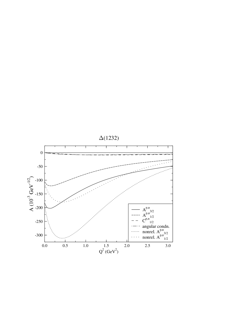
Figure 2: $\Delta(1232)$ electroexcitation helicity amplitudes $A^{p,n}_{3/2}$ (solid curve) and $A^{p,n}_{1/2}$ (dashed curve), and $C^{p,n}_{1/2}$ (long dashes). The dotted curves give the corresponding nonrelativistic results for the Breit-frame transverse helicity amplitudes ($C^{p,n}_{1/2}=0$ in the nonrelativistic model). Also plotted is the value of the rotational covariance condition (dot-dashed curve), which happens to nearly coincide with $C^{p,n}_{1/2}$.

We have also plotted the numerical value of the rotational covariance condition (multiplied by the normalization factor $\zeta\sqrt{4\pi\alpha/2K_{W}}$ for ease of comparison to the physical amplitudes), given by the left-hand side of Eq. (35), for $|\mu^{\prime}-\mu|=2$. At lower values of $Q^{2}$ the rotational covariance condition expectation value is a small fraction of the transverse helicity amplitudes, but approximately the same size as $C_{\textstyle{1\over 2}}$ and larger than the value of $E2/M1$ implied by our $A_{\textstyle{1\over 2}}$ and $A_{\textstyle{3\over 2}}$. Calculations which attempt to predict the ratio using this approach [18] will in general be limited by rotational covariance uncertainties of similar magnitude.

5.2.2 Helicity amplitudes for electroexcitation of radially excited states

Given the controversy surrounding the nature of the baryon states assigned to radial excitations of the nucleon and $\Delta(1232)$ in the nonrelativistic model [25], we compare nonrelativistic and relativistic calculations for simple basis states which can be used to represent the two $P_{11}$ resonances, $N(1440){\textstyle{1\over 2}}^{+}$ and $N(1710){\textstyle{1\over 2}}^{+}$, as well as the $\Delta(1600){\textstyle{3\over 2}}^{+}$, which is assigned as a radial excitation of $\Delta(1232)$ in the nonrelativistic model.

Figure 3 shows our results for the Roper resonance, $N{\textstyle{1\over 2}}^{+}(1440)$, for both proton and neutron targets. Here we have used the single oscillator-basis state Eq. (37) for the initial momentum-space wavefunctions, and a radially excited basis state

$$\Phi^{S^{\prime}}_{0,0}(k_{\rho},K_{\lambda})={1\over\sqrt{3}\pi^{\textstyle{3\over 2}}\alpha_{HO}^{3}}\left(3-[k_{\rho}^{2}+K_{\lambda}^{2}]/\alpha_{HO}^{2}\right){\rm exp}\left\{-[k_{\rho}^{2}+K_{\lambda}^{2}]/2\alpha_{HO}^{2}]\right\}$$ (41)

is used to represent the excited final state. The sign $\zeta$ of the $N\pi$ decays amplitude used here is calculated in the ${}^{3}P_{0}$ model of Ref. [2], using exactly the same wavefunctions. As a consequence, the sign of our nonrelativistic Roper resonance photocouplings calculation [12] disagrees with the sign which appears in Ref. [1], where a reduced matrix element was fit to the sign of the Roper resonance photocouplings.

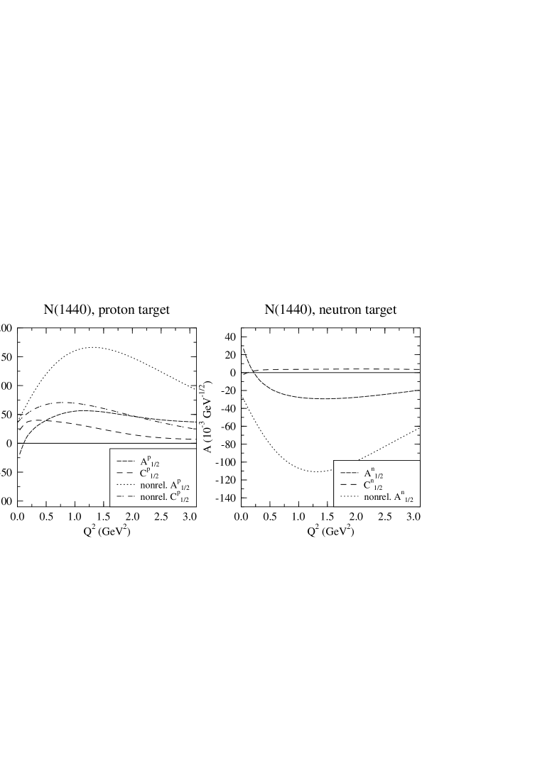
Figure 3: $N(1440)$ electroexcitation helicity amplitudes $A^{p}_{1/2}$ and $A^{n}_{1/2}$ (dashed curves), and $C^{p}_{1/2}$ and $C^{n}_{1/2}$ (long-dashed curves). The dotted curves give the corresponding nonrelativistic result for the Breit-frame transverse helicity amplitudes, and the dot-dashed curve gives the nonrelativistic $C^{p}_{1/2}$ ($C^{n}_{1/2}$ is zero in the nonrelativistic model).

There are large relativistic effects, with differences between the relativistic and nonrelativistic calculations of factors of three or four. Interestingly, the transverse amplitudes also change sign at low $Q^{2}$ values approaching the photon point. The large amplitudes at moderate $Q^{2}$ predicted by the nonrelativistic model (which are disfavored by analyses of the available single-pion electroproduction data [26]) appear to be an artifact of the nonrelativistic approximation. This disagreement, and that of the nonrelativistic photocouplings with those extracted from the data for this state [12], have been taken as evidence that the Roper resonance may not be a simple radial excitation of the quark degrees of freedom but may contain excited glue [27, 28]. The strong sensitivity to relativistic effects demonstrated here suggests that this discrepancy for the Roper resonance amplitudes has a number of possible sources, including relativistic effects.

We also find in the case of proton targets that there is a sizeable $C^{p}_{\textstyle{1\over 2}}$, reaching a value of about $40\times 10^{-3}$ GeV${}^{{\textstyle{1\over 2}}}$ at $Q^{2}$ values between 0.25 and 0.50 GeV². Correspondingly, there will be a sizeable longitudinal excitation amplitude. The nonrelativistic $C^{N}_{\textstyle{1\over 2}}$ amplitudes shown here and in all other figures are listed (up to the $N\pi$ sign $\zeta$) in Appendix C; formulae for the nonrelativistic transverse amplitudes (up to the sign $\zeta$) are tabulated in Ref. [1].

In the case of the $N(1710){\textstyle{1\over 2}}^{+}$, which is assigned a second radially excited wavefunction in the nonrelativistic model, our results using a simple wavefunction made up of a linear combination of basis functions (see Refs. [21] and  [1]) are shown in Fig. 4. Here we see an even greater reduction in the size of the transverse amplitudes in the relativistic calculation. The $C_{1/2}$ amplitudes at the photon point also are greatly reduced in size, although at larger $Q^{2}$ values they become comparable to the nonrelativistic charge helicity amplitudes, with a similar modification of the $Q^{2}$ dependence to that shown above in the case of the Roper resonance and $G^{N}_{E}$.

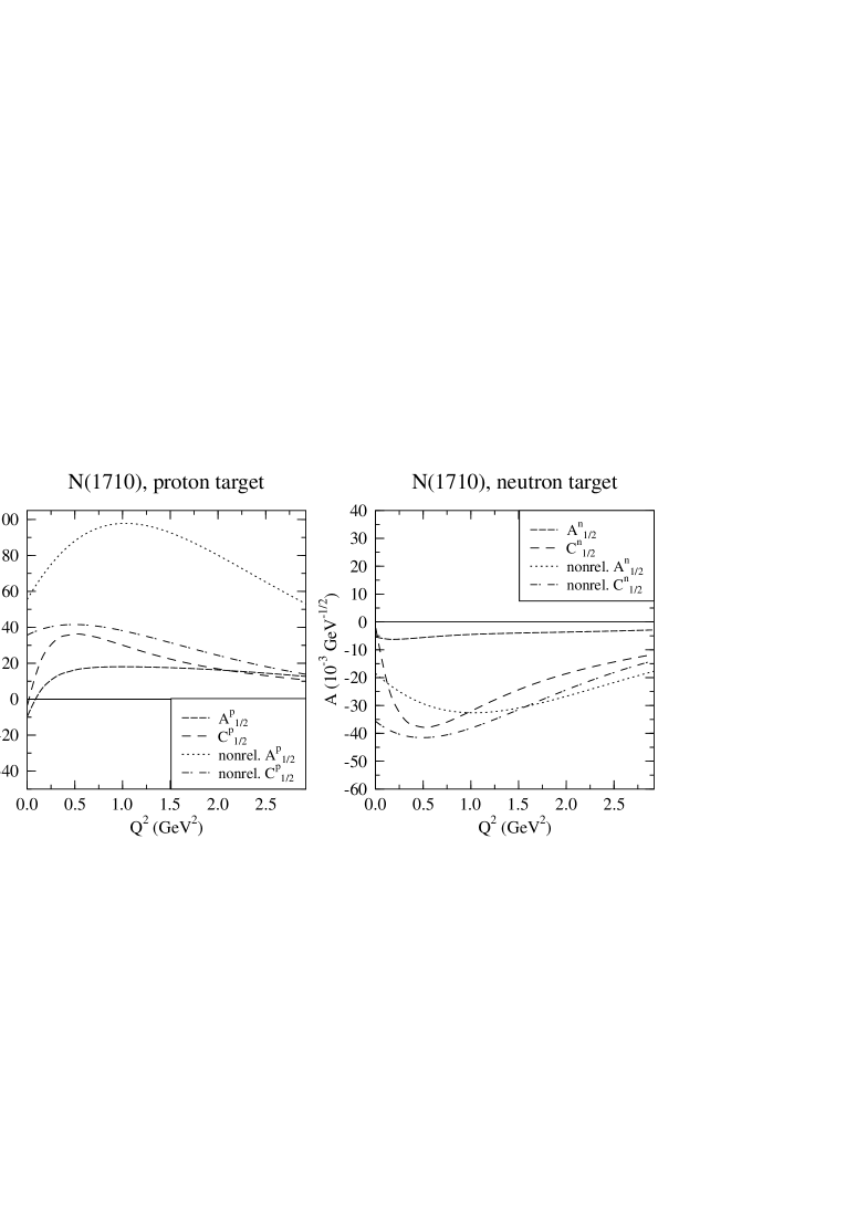
Figure 4: $N(1710$ electroexcitation helicity amplitudes. Key as in Fig. 3, except here the nonrelativistic $C^{n}_{1/2}$ (dot-dashed curve) is nonzero.

It is interesting to see whether this pattern is maintained in the case of the $\Delta(1600){\textstyle{3\over 2}}^{+}$, which has a similar relationship to $\Delta(1232)$ as the Roper resonance has to the nucleon. This is a quark-spin ${\textstyle{3\over 2}}$ state [with spatial wavefunction given by Eq. (41)] in the nonrelativistic model, and so fundamentally differs from the $P_{11}$ states described above. However, examination of the nonrelativistic calculation of the electroexcitation amplitudes shows that in both cases it is the spin-flip part of the O($p/m$) electromagnetic Hamiltonian which is responsible for the transverse transition amplitudes.

This similarity persists in our relativistic calculation (Figure 5), where we see photocouplings which have changed sign in comparison to the nonrelativistic results, along with substantially reduced transverse amplitudes at intermediate $Q^{2}$ values. The falloff with $Q^{2}$ at higher $Q^{2}$ values is quite gradual. As in the case of the $\Delta(1232)$, the relativistic $C_{1/2}$ amplitudes (zero in the nonrelativistic model) are small and comparable in size to the rotational covariance condition, which is generally a small fraction of the transverse amplitudes.

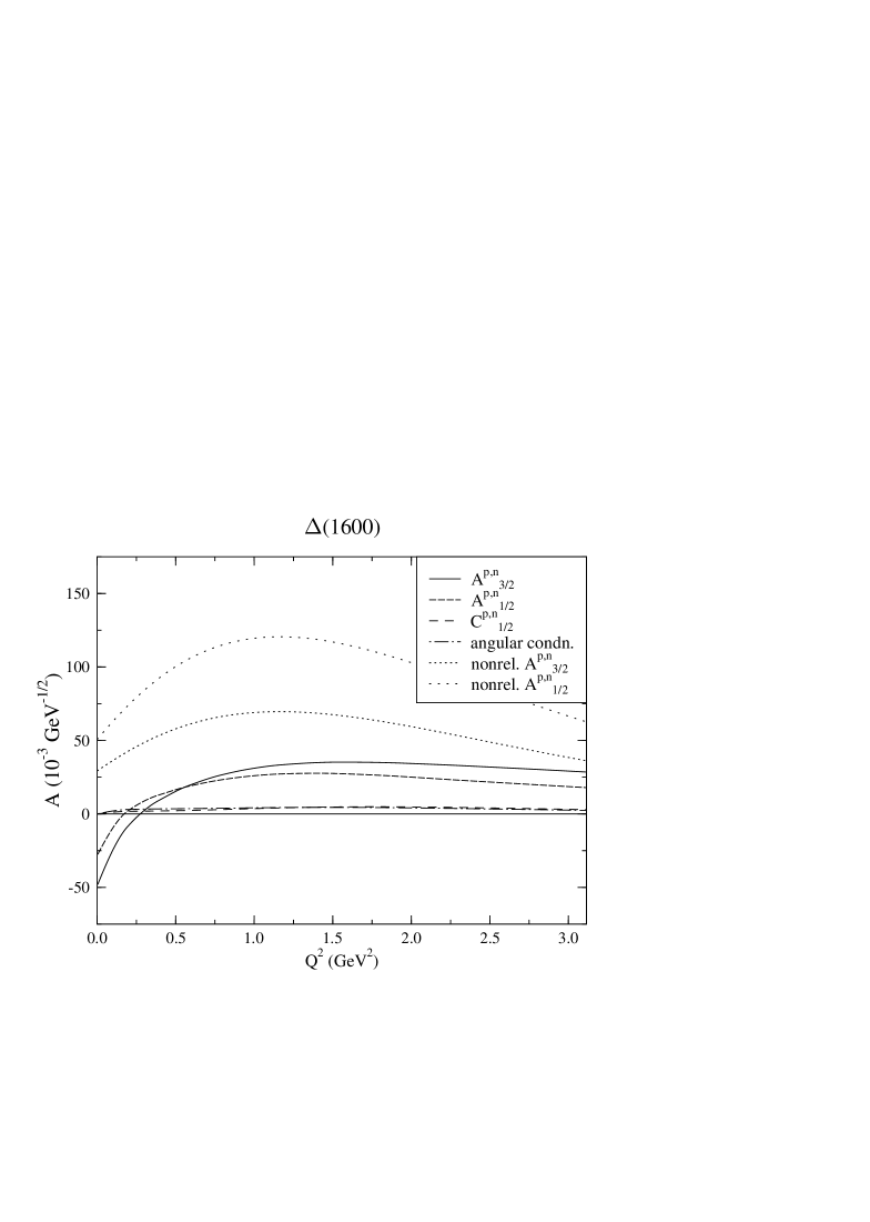
Figure 5: $\Delta(1600)$ electroexcitation helicity amplitudes. Key as in Fig. 2 (here also the nonrelativistic amplitudes $C^{p,n}_{1/2}$ are zero).

5.2.3 Helicity amplitudes for electroexcitation of $P$-wave baryons

We have also calculated helicity amplitudes for the final states $N{\textstyle{3\over 2}}^{-}(1520)$ and $N{\textstyle{1\over 2}}^{-}(1535)$, for both proton and neutron targets. Here we use the same initial-state wavefunction as above and final state wavefunctions which are made up from the orbitally-excited momentum-space wavefunctions

$$\Phi^{M_{\rho}}_{1,+1} = -{1\over\pi^{\textstyle{3\over 2}}\alpha_{HO}^{3}}{k_{\rho+}\over\alpha_{HO}}{\rm exp}\left\{-[k_{\rho}^{2}+K_{\lambda}^{2}]/2\alpha_{HO}^{2}]\right\}$$

$$\Phi^{M_{\lambda}}_{1,+1} = -{1\over\pi^{\textstyle{3\over 2}}\alpha_{HO}^{3}}{K_{\lambda+}\over\alpha_{HO}}{\rm exp}\left\{-[k_{\rho}^{2}+K_{\lambda}^{2}]/2\alpha_{HO}^{2}]\right\},$$ (42)

(where $k_{+}\equiv k_{x}+ik_{y}$) and their counterparts reached by angular momentum lowering. In this case configuration mixing due to the hyperfine interaction is included in the final-state wavefunctions. Since these states are degenerate in mass before the application of spin-spin interactions, they are substantially mixed by them; details are given in Appendix B.

The results for the helicity amplitudes for $N{\textstyle{1\over 2}}^{-}(1535)$ excitation from both proton and neutron targets are compared to the corresponding nonrelativistic results in Figure 6.

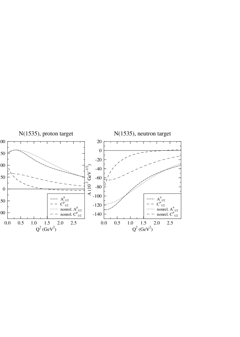
Figure 6: $N(1535)$ electroexcitation helicity amplitudes $A^{p}_{1/2}$ and $A^{n}_{1/2}$ (dashed curves), and $C^{p}_{1/2}$ and $C^{n}_{1/2}$ (long-dashed curves). The dotted and dot-dashed curves give the corresponding nonrelativistic result for the Breit-frame transverse and $C_{1/2}$ helicity amplitudes, respectively.

In contrast to the results shown above, in this case there appears to be little sensitivity to relativistic effects in the results for the transverse amplitudes $A_{1/2}$; this is not the case for the $C_{1/2}$ amplitudes. For both targets there are substantial $C_{1/2}$ amplitudes at small $Q^{2}$, and the $Q^{2}$ dependence is very different in the relativistic calculation (resembling the dipole behavior of the nucleon form factors in Fig. 1).

Our results for the $A_{\textstyle{1\over 2}}$ and $C_{\textstyle{1\over 2}}$ helicity amplitudes for $N{\textstyle{3\over 2}}^{-}(1520)$ excitation from both proton and neutron targets are compared to the nonrelativistic results in Figure 7, and this comparison for $A_{\textstyle{3\over 2}}$ and the value of the rotational covariance condition are shown in Figure 8.

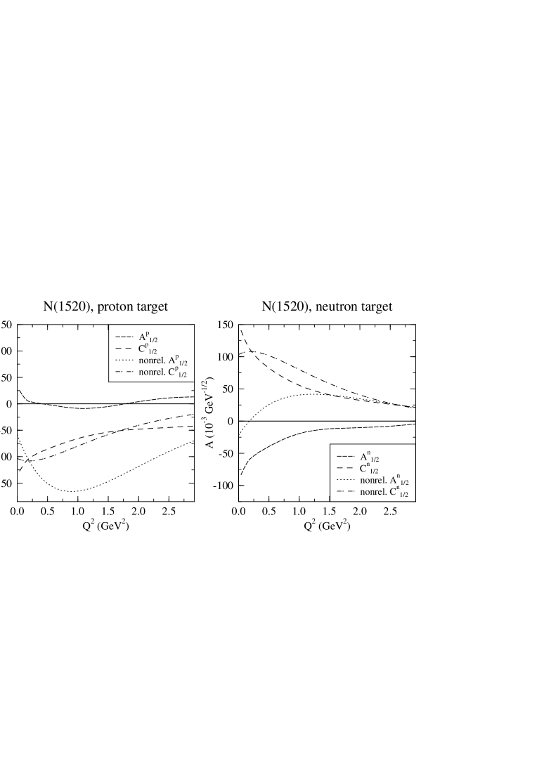
Figure 7: $N(1520)$ electroexcitation helicity-${\textstyle{1\over 2}}$ amplitudes; key as in Fig. 6.

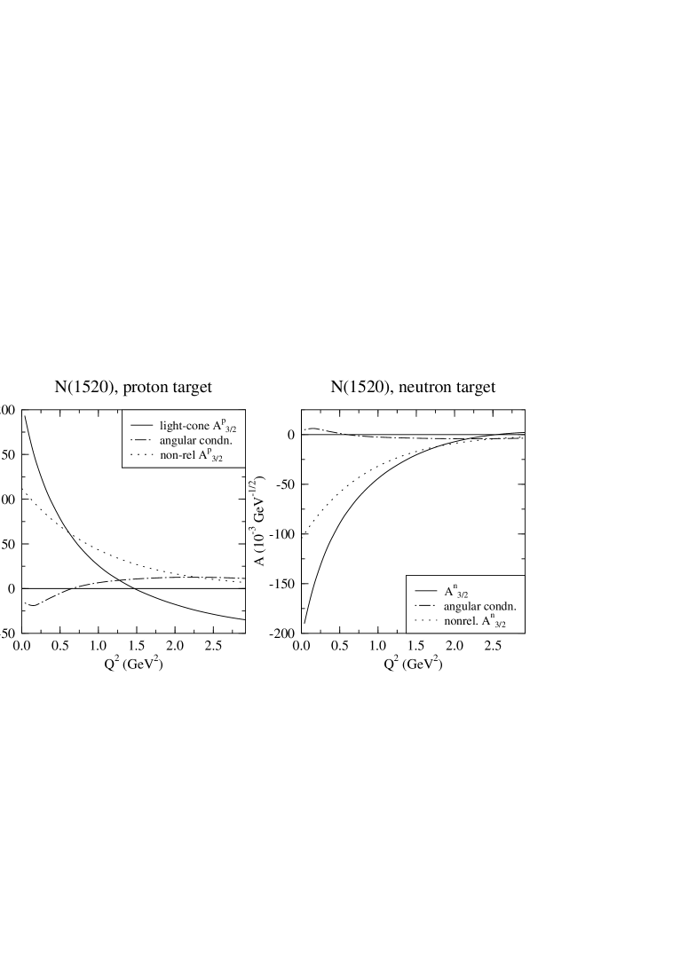
Figure 8: $N(1520)$ electroexcitation helicity amplitudes $A^{p}_{3/2}$ and $A^{n}_{3/2}$ (solid curves), and the value of the rotational covariance condition (dot-dashed curve). The dotted curves give the corresponding nonrelativistic results for the Breit-frame transverse helicity amplitudes.

Here we see large relativistic effects in the $A_{\textstyle{1\over 2}}$ amplitudes. From Ref. [1] one can see that the $A_{\textstyle{1\over 2}}$ amplitudes for this state are proportional to $1-k^{2}/\alpha_{HO}^{2}$ for a proton target, and $1-k^{2}/(3\alpha_{HO}^{2})$ for a neutron target, where $k=|{\bf k}|$ is the virtual-photon three-momentum. Here the constant term arises from the convection part of $H_{\rm em}$, and the $k^{2}/\alpha_{HO}^{2}$ term arises from the quark-spin-flip part. Our relativistic treatment can be expected to change the relationship between these two terms (as well as adding other effects), and we see here that this has caused a substantial cancellation. In this case the charge amplitudes $C_{\textstyle{1\over 2}}$ are greater in magnitude than the transverse amplitudes of both proton and neutron targets, and they are the largest at small $Q^{2}$.

From Fig. 8 we can see that the relativistic effects in $A_{\textstyle{3\over 2}}$ are smaller (in the nonrelativistic model there are not two partially cancelling terms), except near $Q^{2}=0$. In the case of a proton target, the rotational covariance condition expectation value is a substantial fraction of the $A^{p}_{\textstyle{3\over 2}}$ amplitude at larger values of $Q^{2}$, and is comparable to the small $A^{p}_{\textstyle{1\over 2}}$ at all $Q^{2}$ values; the absolute size of the rotational covariance condition can be taken to be a measure of the absolute uncertainty introduced in our results from considerations of rotational covariance.

As an example of a predominantly quark-spin-${\textstyle{3\over 2}}$ P-wave excitation, Fig. 9 shows relativistic and nonrelativistic amplitudes for electroexcitation of $N(1650){\textstyle{1\over 2}}^{-}$, the partner of the predominantly quark-spin-${\textstyle{1\over 2}}$ state $N(1535){\textstyle{1\over 2}}^{-}$ (see Eqs. (53), (54) and (57) in Appendix B).

Figure 9: $N(1650)$ electroexcitation helicity amplitudes. Key as in Fig. 6.

Here, in contrast to those of $N(1535){\textstyle{1\over 2}}^{-}$, the transverse helicity amplitudes show considerable sensitivity to relativistic effects near $Q^{2}=0$ for proton targets, and at all $Q^{2}$ values for neutron targets, and as above the charge helicity amplitudes have remarkably different $Q^{2}$ behavior. Amplitudes for the predominantly quark-spin-${\textstyle{3\over 2}}$ state $N(1700){\textstyle{3\over 2}}^{-}$ tend to be quite small if calculated in the nonrelativistic model [1, 12], and this is still true in our relativistic calculation, with the exception of the amplitude $A^{n}_{\textstyle{3\over 2}}$.

We complete our survey of relativistic effects for basis functions representative of $P$-wave states by examining the amplitudes for electroexcitation of $\Delta(1620){\textstyle{1\over 2}}^{-}$, once again using a simple linear single-oscillator basis wavefunction [Eq. (55) in Appendix B]. Fig. 10 contrasts our results with the nonrelativistic results of Ref. [21] for $A_{\textstyle{1\over 2}}$ and for $C_{\textstyle{1\over 2}}$ from Appendix C. In both cases the amplitudes near $Q^{2}=0$ are considerably larger in the relativistic calculation, with the transverse amplitude decreasing to below the nonrelativistic result above approximately $Q^{2}=0.7$ GeV² due to quite different (dipole-like) behavior as a function of $Q^{2}$. Note in the case of negative-parity $\Delta$ states, the charge helicity amplitudes are not zero if calculated nonrelativistically (see Appendix C). We have found similar relativistic sensitivity in a calculation using a simple basis function which can be used to represent the state $\Delta(1700){\textstyle{3\over 2}}^{-}$.

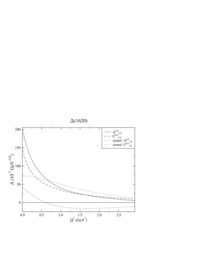
Figure 10: $\Delta(1620)$ electroexcitation helicity amplitudes. Key as in Fig. 6.

6 Discussion and Summary

The results outlined above establish that there will be considerable relativistic effects at all values of $Q^{2}$ in the electroexcitation amplitudes of baryon resonances, even at $Q^{2}=0$. In the real-photon case, this can be understood in terms of the sizeable photon energy required to photoproduce these resonances from the nucleon, which implies a photon three-momentum comparable to the quark Fermi momentum in the nucleon. In particular, our results show that the $Q^{2}$ dependence of the nonrelativistic amplitudes is generally modified into one resembling a dipole falloff behavior, as has been shown in the case of the nucleon form factors. This behavior is likely to be partially modified by the inclusion in the wavefunctions of mixings to higher shells, which are required by any model of baryon structure which takes into account the anharmonic nature of the confining potential between quarks. However, we consider it remarkable that relativistic effects account for a large part of discrepancy between the nonrelativistic model’s predictions and the physical situation.

We wish to stress that the comparisons we have made here, using simple basis functions representing the individual states, are intended to be representative of the degree of sensitivity to relativistic effects for states of their quantum numbers. In order to make reliable predictions for these amplitudes we should use solutions of the relativistic three-body problem; at the very least, configuration mixing of the kind present in the nonrelativistic model must be included in both the nucleon and all of the final states, as it has been shown to have substantial effects on the predicted amplitudes [1, 10, 12]. It is for this reason that we have not compared our results directly to the limited available data [9].

We also note that the Hamiltonian used in Ref. [23] is in fact a three-body mass operator, and so its eigenfunctions can be used directly and consistently in a calculation of the kind described in this paper. We have developed better techniques for performing the numerical integrals required to obtain the light-front matrix elements between configuration-mixed states, whose more complicated integrand structures make standard Monte Carlo methods inefficient.

Nevertheless, it is obvious from the results presented above for radially excited basis states that electroexcitation amplitudes of the $P_{11}$ Roper resonance $N(1440){\textstyle{1\over 2}}^{+}$ and $N(1710){\textstyle{1\over 2}}^{+}$ states, as well as those of the $\Delta(1600){\textstyle{3\over 2}}^{+}$, are substantially modified in a relativistic calculation. Given the controversial nature of these states [27, 28], we consider this an important result. Our results show that relativistic effects tend to reduce the predicted size of the amplitudes for such states at intermediate and high $Q^{2}$ values, in keeping with the limited experimental observations for the best known of these states, $N(1440){\textstyle{1\over 2}}^{+}$.

Within the context of a model such as this one, full gauge invariance cannot be achieved. Reasonable results can be obtained by constraining one of the higher multipoles in terms of lower multipoles. This can be thought of as a variant of the Siegert hypothesis [29], which has been used successfully in the study of electromagnetic properties of nuclei for many years.

We have also found that the rotational covariance violation is a small fraction of the larger amplitudes for the $Q^{2}$ values considered here. In cases where the dynamics causes an amplitude to be intrinsically small, the uncertainty in our results for these amplitudes becomes larger. In particular, the calculated ratios $E2/M1$ and $C2/M1$ for the electroexcitation of the $\Delta(1232){\textstyle{3\over 2}}^{+}$ in the absence of configuration mixing of $D$-wave components into the initial and final state wavefunctions [18] are probably 100% uncertain, and are thus consistent with zero at all $Q^{2}$ [30]. This may not be the case in the presence of such configuration mixing, and we intend to investigate this possibility, since $\Delta(1232)$ electroproduction is the subject of current experiments at MIT/Bates and several proposed experiments at CEBAF [31].

Appendix A: Conventions for Baryon Electroproduction amplitudes

In the following we have collected the information required to translate between standard conventions for (pion) electroproduction amplitudes and our calculated helicity amplitudes.

A.1   Pion electroproduction helicity elements

In the following we relate the helicity elements $A_{l\pm}$, $B_{l\pm}$, and $C_{l\pm}$ conventionally used to describe pion electroproduction to the helicity amplitudes defined above in Eq. (39). The $A_{l\pm}(B_{l\pm})$ elements are present when a resonance is excited by photons with their spin projections antiparallel (parallel) to the target-nucleon spin projection; the momentum of the incoming photon is parallel to the direction of the initial nucleon spin. The $C_{l\pm}$ elements are present when a longitudinal photon excites the resonance (there is no change in the target nucleon spin projection). These can be written in terms of the helicity amplitudes as

$$A_{l\pm} = \mp C^{I}_{\pi N}fA^{N}_{\textstyle{1\over 2}}$$

$$B_{l\pm} = \pm C^{I}_{\pi N}f\sqrt{16\over(2J-1)(2J+3)}A^{N}_{\textstyle{3\over 2}}$$ (43)

$$C_{l\pm} = \mp C^{I}_{\pi N}fC^{N}_{\textstyle{1\over 2}},$$

where $C^{I}_{\pi N}$ is an isospin Clebsch-Gordan coefficient for $N^{*}\to N\pi$, $J$ is the total angular momentum of the resonance $N^{*}$, and $|\vec{k}_{\rm c.m.}|$ is the c.m. frame three-momentum of the photon. The $l$ in the subscripts above is the angular momentum of the relative wavefunction of the final-state $N$ and $\pi$. Note that the $J$ of the resonance must be $J=l\pm{\textstyle{1\over 2}}$, so for a given $J$ there are two possible $l$ values. However only one of these values is consistent with parity conservation. For example for the $\Delta(1232)$ with $J^{P}={\textstyle{3\over 2}}^{+}$ we have $l=1$ or $l=2$, but a nucleon (positive intrinsic parity) and a pion (negative intrinsic parity) in an $l=2$ relative wavefunction have negative overall parity, so this value is not allowed. The sign in the subscripts above is positive if $J=l+{\textstyle{1\over 2}}$ and negative if $J=l-{\textstyle{1\over 2}}$. So for the $\Delta(1232)$ only $A_{1+}$, $B_{1+}$ and $C_{1+}$ are possible.

The Breit-Wigner factor $f$ for the decay $N^{*}\to N\pi$ at resonance is

$$f=\left[{1\over(2J+1)\pi}{K_{W}\over|(\vec{q}_{\pi})_{\rm c.m.}|}{M_{N}\over W}{\Gamma_{N\pi}\over\Gamma_{\rm tot}^{2}}\right]^{\textstyle{1\over 2}},$$ (44)

where $(\vec{q}_{\pi})_{\rm c.m.}$ is the pion c.m. frame three-momentum

$$(\vec{q}_{\pi})_{\rm c.m.}^{2}={[W^{2}-(m_{\pi}+M_{N})^{2}][W^{2}-(m_{\pi}-M_{N})^{2}]\over 4W^{2}}.$$ (45)

With these conventions the $N\gamma$ partial width for a resonance to decay to nucleon $N$ is

$$\Gamma_{N\gamma}={\vec{k}_{\rm c.m.}^{2}\over\pi}{2M_{N}\over(2J+1)W}\left[|A^{N}_{\textstyle{1\over 2}}|^{2}+|A^{N}_{\textstyle{3\over 2}}|^{2}\right].$$ (46)

A.2   Electric, magnetic and scalar multipoles

In the following we relate the magnetic, electric, and scalar/longitudinal multipoles $M_{l\pm}$, $E_{l\pm}$, and $S_{l\pm}$ to the helicity elements described above; these can then be related to the helicity amplitudes calculated here by use of Eq. (43). A transition is defined to be magnetic with multipoles $M_{l\pm}$ if the total angular momentum absorbed from the photon is $l$, and electric with multipoles $E_{l\pm}$ if the total angular momentum absorbed from the photon is $l\pm 1$. The corresponding scalar/longitudinal multipole is $S_{l\pm}$. If $J=l+{\textstyle{1\over 2}}$ the scattering can be described in terms of the magnetic, electric and scalar multipole amplitudes $M_{l+}$, $E_{l+}$, and $S_{l+}$, which can be written in terms of $A_{l+}$, $B_{l+}$ and $C_{l+}$ as

$$M_{l+} = {1\over 2(l+1)}\left[2A_{l+}-(l+2)B_{l+}\right]$$

$$E_{l+} = {1\over 2(l+1)}\left[2A_{l+}+lB_{l+}\right]$$ (47)

$$S_{l+} = {1\over l+1}{|\vec{k}_{\rm c.m.}|\over Q}C_{l+}.$$

If $J=l-{\textstyle{1\over 2}}$ the scattering is described by $M_{l-}$, $E_{l-}$, and $S_{l-}$ with

$$M_{l-} = {1\over 2l}\left[2A_{l-}+(l-1)B_{l-}\right]$$

$$E_{l-} = {1\over 2l}\left[-2A_{l-}+(l+1)B_{l-}\right]$$ (48)

$$S_{l-} = -{1\over l}{|\vec{k}_{\rm c.m.}|\over Q}C_{l-}.$$

The inverse transformation is

$$A_{l+} = {1\over 2}\left[lM_{l+}+(l+2)E_{l+}\right]$$

$$B_{l+} = -M_{l+}+E_{l+}$$ (49)

$$A_{l-} = {1\over 2}\left[(l+1)M_{l-}-(l-1)E_{l-}\right]$$

$$B_{l-} = M_{-}+E_{l-}.$$

A.3   Invariant multipoles for $\Delta(1232)$ electroproduction

For the special case of electroproduction of a $J^{P}={\textstyle{3\over 2}}^{+}$ particle such as the $\Delta{\textstyle{3\over 2}}^{+}(1232)$, we can define invariant multipoles $G^{*}_{M}$, $G^{*}_{E}$ and $G^{*}_{C}$. The relation between these and the helicity amplitudes defined above is

$$G^{*}_{M} = -F\left[\sqrt{3}A^{N}_{\textstyle{3\over 2}}+A^{N}_{\textstyle{1\over 2}}\right]$$

$$G^{*}_{E} = -F\left[{1\over\sqrt{3}}A^{N}_{\textstyle{3\over 2}}-A^{N}_{\textstyle{1\over 2}}\right]$$ (50)

$$G^{*}_{C} = 2{W\over|\vec{k}_{\rm c.m.}|}F\sqrt{2}S^{N}_{\textstyle{1\over 2}},$$

where

$$F=\sqrt{{1\over 4\pi\alpha}{M_{N}\over W}K_{W}}\left[1+{Q^{2}\over(M_{N}+W)^{2}}\right]^{\textstyle{1\over 2}}{M_{N}\over|\vec{k}_{\rm c.m.}|}.$$ (51)

Note that Eq. (51) implies that at the photoproduction point ($Q^{2}=0$, where $|\vec{k}_{\rm c.m.}|=K_{W}$) we have

$$F(0)=\sqrt{1\over 4\pi\alpha}\sqrt{2M_{N}^{3}\over W^{2}-M_{N}^{2}}.$$ (52)

Appendix B: Wavefunctions for the $P$-wave baryons

We construct $N$ and $\Delta$ states which have the correct permutational symmetry (mixed-$\lambda$ type for $N$ states, and symmetric for $\Delta$ states) in their flavor/spin/space wavefunctions. A common totally antisymmetric color wavefunction is assumed, as is an implicit Clebsch-Gordan sum coupling ${\bf L}$ and ${\bf S}$. The spin-quartet $N$ states (notation is $|F^{2S+1}L_{\sigma}J^{P}\rangle$, with $F$ the flavor $N$ or $\Delta$, and $\sigma$ the spatial permutational symmetry) $|N^{4}P_{M}{\textstyle{1\over 2}}^{-}\rangle$, $|N^{4}P_{M}{\textstyle{3\over 2}}^{-}\rangle$, and $|N^{4}P_{M}{\textstyle{5\over 2}}^{-}\rangle$ are made up of Clebsch-Gordan linear combinations of

$$uud\chi^{S}_{{\textstyle{3\over 2}},\mu}\Psi^{\lambda}_{1,M}\ .$$ (53)

The spin-doublet $N$ states $|N^{2}P_{M}{\textstyle{1\over 2}}^{-}\rangle$ and $|N^{2}P_{M}{\textstyle{3\over 2}}^{-}\rangle$ are made from

$$uud{1\over\sqrt{2}}\left(\chi^{\rho}_{{\textstyle{1\over 2}},\mu}\Psi^{\rho}_{1,M}-\chi^{\lambda}_{{\textstyle{1\over 2}},\mu}\Psi^{\lambda}_{1,M}\right),$$ (54)

and the spin-doublet $\Delta$ states $|\Delta^{2}P_{M}{\textstyle{1\over 2}}^{-}\rangle$ and $|\Delta^{2}P_{M}{\textstyle{3\over 2}}^{-}\rangle$ are made from

$$uud{1\over\sqrt{2}}\left(\chi^{\rho}_{{\textstyle{1\over 2}},\mu}\Psi^{\rho}_{1,M}+\chi^{\lambda}_{{\textstyle{1\over 2}},\mu}\Psi^{\lambda}_{1,M}\right).$$ (55)

Where mixing is allowed, the physical states do not have definite quark spin $S$. We have used [21]

$$|N(1535){\textstyle{1\over 2}}^{-}\rangle \to \phantom{-}0.85|N^{2}P_{M}{\textstyle{1\over 2}}^{-}\rangle+0.53|N^{4}P_{M}{\textstyle{1\over 2}}^{-}\rangle$$

$$|N(1650){\textstyle{1\over 2}}^{-}\rangle \to -0.53|N^{2}P_{M}{\textstyle{1\over 2}}^{-}\rangle+0.85|N^{4}P_{M}{\textstyle{1\over 2}}^{-}\rangle$$

$$|N(1520){\textstyle{3\over 2}}^{-}\rangle \to \phantom{-}0.99|N^{2}P_{M}{\textstyle{3\over 2}}^{-}\rangle-0.11|N^{4}P_{M}{\textstyle{3\over 2}}^{-}\rangle$$ (56)

$$|N(1700){\textstyle{3\over 2}}^{-}\rangle \to \phantom{-}0.11|N^{2}P_{M}{\textstyle{3\over 2}}^{-}\rangle+0.99|N^{4}P_{M}{\textstyle{3\over 2}}^{-}\rangle.$$ (57)

Appendix C: Nonrelativistic $C^{N}_{\textstyle{1\over 2}}$ amplitudes for electroexcitation of resonances

In the Figures above we have plotted predictions of the Isgur-Karl-Koniuk (nonrelativistic) model for the charge helicity amplitudes $C^{p}_{\textstyle{1\over 2}}$ and $C^{n}_{\textstyle{1\over 2}}$. To the best of our knowledge these are not published elsewhere, so we list them below.

For $N{\textstyle{1\over 2}}^{+}(1440)$,

$$C^{(p,n)}_{\textstyle{1\over 2}}=A_{0}\left[-{\sqrt{3}k^{2}m_{q}\over 9\alpha_{HO}^{2}}\right](1,0),$$ (58)

where

$$A_{0}=\sqrt{2\pi\over k_{0}}{e\over 2m_{q}}e^{-k^{2}/(6\alpha_{HO}^{2})},$$ (59)

and $(k_{0},{\bf k})$, with $k=|{\bf k}|$, is the (virtual) photon four-momentum in the frame in which the calculation is performed (taken here to be the Breit frame). For the states $N(1535){\textstyle{1\over 2}}^{-}$ and $N(1650){\textstyle{1\over 2}}^{-}$ we give the amplitudes for their two components $N^{2}P_{M}{\textstyle{1\over 2}}^{-}$ and $N^{4}P_{M}{\textstyle{1\over 2}}^{-}$,

$$C^{(p,n)}_{\textstyle{1\over 2}}(N^{2}P_{M}{\textstyle{1\over 2}}^{-}) = A_{0}\left[i{\sqrt{2}km_{q}\over 3\alpha_{HO}}\right](1,-1),$$ (60)

$$C^{(p,n)}_{\textstyle{1\over 2}}(N^{4}P_{M}{\textstyle{1\over 2}}^{-}) = 0,$$

and similarly for the states $N(1520){\textstyle{3\over 2}}^{-}$ and $N(1700){\textstyle{3\over 2}}^{-}$

$$C^{(p,n)}_{\textstyle{1\over 2}}(N^{2}P_{M}{\textstyle{1\over 2}}^{-}) = A_{0}\left[i{2km_{q}\over 3\alpha_{HO}}\right](-1,1),$$ (61)

$$C^{(p,n)}_{\textstyle{1\over 2}}(N^{4}P_{M}{\textstyle{1\over 2}}^{-}) = 0.$$

For $\Delta{\textstyle{1\over 2}}^{-}(1620)$

$$C^{N}_{\textstyle{1\over 2}}=-A_{0}i{\sqrt{2}km_{q}\over 3\alpha_{HO}},$$ (62)

and for $\Delta{\textstyle{3\over 2}}^{-}(1700)$

$$C^{N}_{\textstyle{1\over 2}}=A_{0}i{2km_{q}\over 3\alpha_{HO}}.$$ (63)

For $N{\textstyle{1\over 2}}^{+}(1710)$,

$$C^{(p,n)}_{\textstyle{1\over 2}}=A_{0}\left[{\sqrt{6}k^{2}m_{q}\over 18\alpha_{HO}^{2}}\right](1,-1).$$ (64)

References

- [1] R. Koniuk and N. Isgur, Phys. Rev. D21, 1868 (1980)
- [2] S. Capstick and W. Roberts, Phys. Rev. D47, 1994 (1993); Phys. Rev. D49, 4570 (1994).
- [3] C. Hayne and N. Isgur, Phys. Rev. D25, 1944 (1980); D.P. Stanley and D. Robson, Phys. Rev. D26, 223 (1982).
- [4] P.-L. Chung and F. Coester, Phys. Rev. D44, 229 (1991).
- [5] F. Schlumpf, Mod. Phys. Lett. A8, 2135 (1993); J. Phys. G20, 237 (1994); Zurich University doctoral thesis, RX-1421 (Zurich), 1992.
- [6] H.J. Weber, Phys. Lett. B287, 14 (1992); Phys. Rev D41, 2201 (1992); Ann. Phys. 177, 38 (1987).
- [7] See I.G. Aznaurian, Phys. Lett. 316B, 391 (1993), and references therein.
- [8] S. Capstick and G. Karl, Phys. Rev. D41, 2767 (1990).
- [9] V.D. Burkert, in the proceedings of Excited Baryons 1988 (Troy, New York, August 1988), World Scientific, Eds. G. Adams, N. C. Mukhopadhyay, Paul Stoler, pp. 122; V.D. Burkert, Int. J. Mod. Phys. E1, 421 (1992).
- [10] F.E. Close and Zhenping Li, Phys. Rev. D42, 2194 (1990); Zhenping Li and F.E. Close, D42, 2207 (1990).
- [11] M. Warns, H. Schröder, W.P. Pfeil, and H. Rollnik, Zeit. Phys. C45, 613 (1990); C45, 627 (1990); M. Warns, W. Pfeil, and H. Rollnik, Phys. Rev. D42, 2215 (1990).
- [12] S. Capstick, Phys. Rev. D46, 1965 (1992); D46, 2864 (1992).
- [13] See, for example, W. Glöckle, T.-S. H. Lee and F. Coester, Phys. Rev C33, 709 (1986).
- [14] H.-C. Jean, S. Capstick, B.D. Keister, and D. Robson, work in progress.
- [15] B. D. Keister and W. N. Polyzou, Adv. Nucl. Phys. 20, 225 (1991).
- [16] B. D. Keister, Phys. Rev. D49, 1500 (1994).
- [17] H.J. Weber, Ann. Phys. 207, 417 (1991).
- [18] J. Bienkowska, Z. Dziembowski, and H.J. Weber, Phys. Rev. Lett. 59, 624 (1987); ibid 59E 1790 (1987).
- [19] H.J. Weber, Phys. Rev. D41, 2201 (1990).
- [20] H. J. Melosh Phys. Rev. D9, 1095 (1974).
- [21] N. Isgur and G. Karl, Phys. Rev. D18, 4187 (1978); Phys. Rev. D19, 2653 (1979).
- [22] G. P. Lepage, J. Comp. Phys. 27, 192 (1978).
- [23] S. Capstick and N. Isgur, Phys. Rev. D34, 2809 (1986).
- [24] F. Foster and G. Hughes, Rep. Prog. Phys. 46, 1445 (1983).
- [25] See, for example, Ref. [12], and references therein.
- [26] P. Stoler, Phys. Rep. 226 103 (1993).
- [27] Z.-P. Li, Phys. Rev. D44, 2841 (1991).
- [28] Z.-P. Li. V. Burkert, and Z.-J. Li, Phys. Rev. D46, 70 (1992).
- [29] A.J.F. Siegert, Phys. Rev. 52, 787 (1937).
- [30] Although it may not be obvious from Fig. 2, our results for the transverse amplitudes at yield E2/M1 and C2/M1 which are exactly zero.
- [31] V. Burkert et al., CEBAF proposal PR-89-037, ; P. Stoler et al., CEBAF proposal PR-91-002; S. Frullani et al., CEBAF proposal PR-91-011; J. Napolitano, P. Stoler et al., CEBAF Experiment E94-14.