LUNFD6/(NFFL-7084) 1994

nucl-th/9408022

Quantum Statistical Correlations for
Slowly Expanding Systems

T. Csörgő^1,2 B. Lörstad^2,∗ and J. Zimányi^1,∗

¹KFKI Research Institute for Particle and Nuclear Physics of the
Hungarian Academy of Sciences, H–1525 Budapest 114, P.O. Box 49. Hungary
²Department of Elementary Particle Physics, Physics Institute,
University of Lund, Sölvegatan 14, S - 223 62 Lund, Sweden

Abstract

Quantum statistical correlations and momentum distributions are calculated for a spherically symmetric, three-dimensionally expanding finite fireballs, for non-relativistic expansions applying plane-wave approximation. The new concepts of the geometrical temperature as well as the thermal radius are presented for the simplest case. The symmetry properties of the correlation function are shown to reflect the symmetry properties of the emission function.

Accepted for publication in Phys. Lett. B

Intensity interferometry has recently become a popular tool to infer the freeze-out surface heavy ion collisions and to study the space-time characteristics of the strong interactions in elementary particle reactions. The method was originally invented  [1] to measure the angular diameter of distant stars or galaxies, the investigated objects being approximately static and the length-scales astronomical. In principle the same method is applied to measure the space-time characteristics of the strong interaction, where the objects under study are expanding systems, with life-times of a few fm/c ($10^{-23}$ sec) and length-scales of a few fm ($10^{-15}$ m).

In recent publications [2, 3] the new concept of the geometrical temperature and also the concept of thermally generated length-scales [4, 5, 2, 3] were introduced for relativistically expanding systems both in one and three dimensions. In ref. [3] application for recent high energy heavy ion data from the CERN energy region  [6, 7] was found: for three-dimensionally expanding, cylindrically symmetric, finite systems the Bose-Einstein Correlation Function (BECF) was shown to measure the thermal length scale, the region in the coordinate-space from where bosons with similar momenta may emerge. The size of this region is determined by the freeze-out temperature, the freeze-out time and the flow gradients. It was shown that this thermal length-scale dominates the correlation function if the geometrical characteristic length scales are sufficiently large. However, the $m_{t}$ dependence of the parameters of the BECF were shown to contain correction terms proportional to the ratio of the thermal/geometrical length scales. As a complementary effect, the momentum distribution was shown to be dominated by the geometrical and not the thermal parameters, which provides us a possibility to measure the (large) geometrical scales by a systematic study of the single-particle momentum distribution. These effects appear for thermal lengths small compared to the geometrical size of the expanding system. The standard results  [8, 9] are reproduced for the case the geometrical length-scales being smaller than the thermal ones: in this conventional case the BECF measures the geometrical size properly and the freeze-out temperature can be extracted from the momentum distribution.

The motivation for the present Letter is to investigate how the thermal lengths and the geometrical temperature reveal themself for the simplest systems where they appear at all. Since the thermal length-scales appear due the interplay of the flow-gradient and the temperature, a non-relativistically expanding thermal source with constant flow-gradient is the simplest possible case. The key feature is that the Bose-Einstein or Fermi-Dirac correlations appear due to an enhanced/decreased probability of finding identical particles in a similar momentum-state; i. e. the correlations vanish for large momentum difference. In case of an expanding source with flow gradients, the mean momentum of the emitted particles changes with changing locations. Locally, the width of the momentum distribution of the emitted particles is determined by the temperature; thus there will be a region in the coordinate space, where the change in the mean momentum of the emitted particles is of the same magnitude as the width of the local momentum distribution. The size of this region is referred to as the thermal length. If it is smaller than the geometrical size of the expanding system, the quantum statistical correlations (Bose-Einstein or Fermi-Dirac) shall be sensitive only to this thermal size, since this is the size of the coordinate-space from which particles with similar momenta may emerge.

Thus the simplest case is a non-relativistic expansion with constant gradient. We may choose the case of the three-dimensionally expanding, finite systems with spherical symmetry, which is most probably realized in low energy heavy ion collisions. For a recent review on the intensity interferometry of low and intermediate energy heavy ion collisions (E/A $<$ 1 GeV) see ref. [10].

The particle emission is characterized by the emission function $S(x,p)$ which is the probability that a particle is produced at a given $x=(t,\vec{r}\,)=(t,x,y,z)$ point in space-time with the four-momentum $p=(E,\vec{p}\,)=(E,p_{x},p_{y},p_{z})$, where the particle is on mass shell, $m^{2}=E^{2}-\vec{p}^{\,\,2}$. The quantum-mechanical analogy to the classical emission function is the time-derivative of the Wigner-function, [11].

In terms of the time derivative of the Wigner-function both the momentum spectra and the quantum statistical correlation functions (QSCF-s) are prescribed. A useful auxiliary function is the Fourier-transformed emission function

$$\tilde{S}(\Delta k,K) = \int d^{4}x\,\,S(x,K)\,\exp(i\Delta k\cdot x),$$ (1)

where

$$\Delta k=p_{1}-p_{2}, K={\displaystyle p_{1}+p_{2}\over\displaystyle 2}$$ and (2)

and $\Delta k\cdot x$ stands for the inner product of the four-vectors. Then the momentum distribution of the emitted particles, $f(p)$ is given by

$$f(p) = \tilde{S}(\Delta k=0,K=p),$$ (3)

which is normalized to unity,

$$\int d^{3}p\,\,f(p) = 1.$$ (4)

The two-particle Bose-Einstein or Fermi-Dirac correlation functions (BECF-s or FDCF-s) are prescribed in terms of our auxiliary function,

$$C(K,\Delta k) = 1\pm{\displaystyle\mid\tilde{S}(\Delta k,K)\mid^{2}\over\displaystyle\mid\tilde{S}(0,K)\mid^{2}},$$ (5)

where the $+$ sign stands for bosons and the $-$ sign for fermions, as was presented e.g. in ref. [11, 9]. In this Letter the effect of final state Coulomb and Yukawa interactions shall be neglected as implicitly assumed by the above equation, and the time-derivative of the Wigner-function shall be approximated by classical emission functions. We assume completely chaotic, thermal emission. For Fermi-Dirac correlations, the plane-wave approximation is rather crude especially due to the attractive final state interactions in $pp$ and $nn$ systems for which systems a large data set was taken at low and intermediate energies [10]. The Coulomb repulsion in the $pp$ channel plays also an important role. These final state interactions can be taken into account in the Wigner-function formalism along the lines of ref. [11]. The Fourier-transformations which appear in this Letter are the consequence of the plane-wave approximation for the relative wave-function $\psi_{\Delta k}(\vec{r},t)$. They correspond to integrals over $\mid\psi_{\Delta k}(\vec{r},t)\mid^{2}=1+\cos(\Delta k\cdot x)$. In the case the final state interactions are taken into account, the Fourier-transformations are to be replaced by integral transformations over the $\phi_{\Delta k}(\vec{r},t)$ relative wave function which can be calculated for the Coulomb + Yukawa final state interactions as mentioned e.g. in  [11].

For central heavy ion collisions at low or intermediate energies the target and the projectile form a collective state (stopping) which can be described as a non-relativistically expanding fluid within the framework of hydrodynamical models. Due to the expansion, the fluid cools and at a certain temperature it freezes out. In case of full stopping and thermalization (spherically symmetric momentum distribution) the information about the initial direction is lost thus the final freeze-out density distribution becomes approximately spherically symmetric, too.

We shall assume that the emission function is characterized by a given a distribution of production points $I(\vec{r}\,\,)$ and by a distribution of the freeze-out times, $H(t)$. The correlations between space-time and momentum-space shall be introduced by a non-relativistic momentum distribution. We assume that the expanding system at the freeze-out is rare enough so that the quantum-statistical single-particle distribution can be well approximated by a Boltzmann-distribution,

$$f_{B}(x;p) = C\exp\left(-{\displaystyle(\vec{p}-m\vec{u}(x))^{2}\over\displaystyle 2mT}\right).$$ (6)

Here $\vec{u}(x)$ is the (non-relativistic) velocity, the freeze-out temperature is denoted by $T$ and the quantity $C={\displaystyle 1\over\displaystyle(2\pi mT)^{3/2}}$ is a normalization constant. Thus the emission function is characterized as

$$S(x;K) = f_{B}(x;K)\,I(\vec{r}\,)\,H(t).$$ (7)

In order to simplify the results we keep only the mean value and the width of the source distributions i.e. we shall apply Gaussian approximations for the distribution functions of $t$ and $\vec{r}$ as follows

$$I(\vec{r}\,) = {\displaystyle 1\over\displaystyle(2\pi R_{G}^{2})}\,\exp\left(-{\displaystyle{\vec{r}\,}^{2}\over\displaystyle 2R_{G}^{2}}\right)$$ (8)

$$H(t) = {\displaystyle 1\over\displaystyle(2\pi\Delta t^{2})^{1/2}}\,\exp\left(-{\displaystyle(t-t_{0})^{2}\over\displaystyle 2\Delta t^{2}}\right).$$ (9)

We shall also briefly discuss our results for the general case.

We select a velocity of the 3D expanding matter at space-time point $x$ so that it be spherically symmetric and describe an expansion in all three directions with a constant gradient. Thus the velocity around the mean freeze-out time $t_{0}$ is assumed to have the form

$$\vec{u}(x) = {\displaystyle\vec{r}\over\displaystyle t_{0}},$$ (10)

which describes a scaling solution of the non-relativistic hydrodynamical equations at the mean freeze-out time $t_{0}$ for $r<<t_{0}$, ref. [12]. Further we assume that the freeze-out temperature in this non-relativistic case is smaller than the mass of the particles, $T<m$.

With the help of the above flow pattern, the Boltzmann factor at the mean freeze-out time can be rewritten as

$$J(\vec{r}-\vec{r}_{a}\,) = f_{B}(t_{0},\vec{r}\,;K)\,=\,C\exp\left(-{\displaystyle\left(\vec{r}-\vec{r}_{a}(K)\right)^{2}\over\displaystyle 2R_{T}^{2}}\right)$$ (11)

i.e. the emission of the particles with momentum $K$ is characterized by a Gaussian. The mean emission point $\vec{r}_{a}(K)$ is proportional to the observed momentum and the width of the emission points around the mean is determined by the mean freeze-out time (inverse of the velocity gradient) and the freeze-out temperature:

$$\vec{r}_{a}(K)={\displaystyle t_{0}\over\displaystyle m}\vec{K}, R_{T}^{2}=t_{0}^{2}{T\over\displaystyle m}.$$ (12)

This width $R_{T}$ shall be referred to as the ’thermal radius’.

When these approximations are valid, our auxiliary function can be rewritten as

$$\tilde{S}(\Delta k,K) = \tilde{H}(\Delta E)\int d^{3}\vec{r}\,\exp\left(\,-i\,\Delta\vec{k}\,\vec{r}\,\right)\,\,I(\vec{r}\,)\,\,J(\vec{r}-t_{0}{\displaystyle\vec{K}\over\displaystyle m}),$$ (13)

where $\tilde{H}(\Delta E)$ stands for the Fourier-transformed freeze-out time distribution. Let’s introduce the effective, $\vec{K}$ dependent particle emission function

$$I^{eff}_{K}(\vec{r}\,) = I(\vec{r}\,)\,\,J(\vec{r}-t_{0}{\displaystyle\vec{K}\over\displaystyle m}\,).$$ (14)

Thus for arbitrary, Fourier-transformable distributions the momentum distribution and the QSCF is given as

$${\displaystyle d^{3}n\over\displaystyle dp_{x}dp_{y}dp_{z}} \propto f(\vec{p}\,)=\int d^{3}\vec{r}\,\,I^{eff}_{p}(r)\,=$$ (15)

$$= \int d^{3}\vec{r}\,\,I(\vec{r}\,)\,\,J(\vec{r}-t_{0}{\displaystyle\vec{p}\over\displaystyle m}\,),$$ (16)

$$C(\vec{K},\Delta\vec{k}) = 1\pm\mid\tilde{H}(\Delta E)\mid^{2}{\displaystyle\mid\tilde{I}^{eff}_{K}(\Delta\vec{k}\,)\mid^{2}\over\displaystyle\mid\tilde{I}^{eff}_{K}(\,0\,)\mid^{2}}$$ (17)

Thus the momentum distribution is given by a convolution and the QSCF shall be a symmetric function in the CMS of the pair, where $\Delta E=0$.

These general results take particularly simple form in the introduced Gaussian approximations. The auxiliary function $\tilde{S}(\Delta k,K)$ contains a factor which is the Fourier-transform of the product of Gaussians and so easily integrable. The two Gaussian factors can be combined into a single Gaussian by introducing the following notation:

$${\displaystyle(\vec{r}-\vec{r}_{a})^{2}\over\displaystyle R_{T}^{2}}+{\displaystyle\vec{r}\,^{2}\over\displaystyle R_{G}^{2}} = {\displaystyle(\vec{r}-\vec{r}_{b})^{2}+\vec{r}_{c}\,^{2}\over\displaystyle R_{*}^{2}},$$ (18)

and the new variables can be determined by the requirement that the coefficients of the powers of $\vec{r}$ should be equal on both sides. This yields the following relations:

$${\displaystyle 1\over\displaystyle R_{*}^{2}} = {\displaystyle 1\over\displaystyle R_{T}^{2}}+{\displaystyle 1\over\displaystyle R_{G}^{2}},$$ (19)

$${\displaystyle\vec{r}_{a}\over\displaystyle R_{T}^{2}} = {\displaystyle\vec{r}_{b}\over\displaystyle R_{*}^{2}},$$ (20)

$${\displaystyle\vec{r}_{a}\,^{2}\over\displaystyle R_{T}^{2}} = {\displaystyle\vec{r}_{b}\,^{2}+\vec{r}_{c}\,^{2}\over\displaystyle R_{*}^{2}},$$ (21)

and now the factor $\exp\left(-{\displaystyle\vec{r}_{c}\,^{2}\over\displaystyle 2R_{*}^{2}}\right)$ becomes independent of the integration. This factor shall enter the momentum distribution and can be rewritten as

$$\exp\left(-{\displaystyle\vec{K}^{2}\over\displaystyle 2mT_{*}}\right),$$ (22)

where the effective temperature $T_{*}$ is the sum of the freeze-out temperature and the ”geometrical temperature”,

$$T_{*}=T+T_{G}, T_{G}=m{\displaystyle R_{G}^{2}\over\displaystyle t_{0}^{2}}.$$ where (23)

The last line defines the geometrical temperature, being just the mass multiplied by the square of the mean expansion velocity ${\displaystyle R_{G}\over\displaystyle t_{0}}$. The geometrical temperature $T_{G}$ is related to the geometrical radius $R_{G}$ exactly the same way as the freeze-out temperature $T$ is related to the thermal radius $R_{T}$:

$$R_{G}^{2} = t_{0}^{2}{\displaystyle T_{G}\over\displaystyle m},$$ (24)

$$R_{T}^{2} = t_{0}^{2}{\displaystyle T\over\displaystyle m}.$$ (25)

The remaining integral in the auxiliary function is trivial, resulting in the following momentum-distribution and correlation function:

$$f(\vec{p}\,) = {\displaystyle 1\over\displaystyle(2\pi mT_{*})^{3/2}}\exp\left(-{\displaystyle\vec{p}\,^{2}\over\displaystyle 2mT_{*}}\right),$$ (26)

$$C(\vec{K},\Delta\vec{k}\,) = 1\pm\exp(-R_{*}^{2}\Delta\vec{k}^{2})\,\exp(-\Delta t^{2}\Delta E^{2}).$$ (27)

The effective temperature $T_{*}$ and the effective radius parameter, $R_{*}$ were defined in eqs. 19,23.

The relative momentum $\Delta\vec{k}$, which enters the correlation function, is invariant under Galilei-transformations. However, the energy difference is not invariant even under the non-relativistic Galilei transformations. Let us re-formulate $\Delta E$ in such a way that its specific directional dependence be more transparent. The energy difference could be identically rewritten as

$$\Delta E^{2}={\displaystyle\vec{p}_{1}\,^{2}-\vec{p}_{2}\,^{2}\over\displaystyle 2m} = \left({\displaystyle\vec{p}_{1}+\vec{p}_{2}\over\displaystyle 2}\right){\displaystyle\Delta\vec{k}\over\displaystyle m}=\vec{v}_{K}\Delta\vec{k},$$ (28)

where we have introduced the mean velocity of the pair, $\vec{v}_{K}={\displaystyle\vec{p}_{1}+\vec{p}_{2}\over\displaystyle 2m}={\displaystyle\vec{K}\over\displaystyle m}$.

Let us define the out direction to be parallel to the mean velocity of the pair, $\vec{v}_{K}$, and the perp index shall be used to index the remaining two principal directions, both being perpendicular to the out direction. This naming convention corresponds to the one used in high energy heavy ion collisions [13, 5].

By this definition we evaluate the correlation function in a frame which is assigned to a given mean momentum of the particle pair and not that of the fireball: by changing the mean momentum we change our reference frame too. In this co-moving frame the relative momentum is decomposed as

$$\Delta\vec{k}=(Q_{out},\vec{Q}_{perp})$$ (29)

and the correlation function can be rewritten as

$$C(Q_{out},Q_{perp}) = 1\pm\exp\left(-R_{perp}^{2}Q_{perp}^{2}-R_{out}^{2}Q_{out}^{2}\right),$$ (30)

$$R_{perp}^{2} = R_{*}^{2}={\displaystyle R_{T}^{2}R_{G}^{2}\over\displaystyle R_{T}^{2}+R_{G}^{2}},$$ (31)

$$R_{out}^{2} = R_{*}^{2}+\vec{v}_{K}\,^{2}\Delta t^{2}.$$ (32)

Thus the perpendicular components shall measure the effective radius $R_{*}$. What is the interpretation of this quantity?

There are two length-scales in the problem: the geometrical length-scale $R_{G}$ and the thermal one $R_{T}$, the latter being generated by the flow-gradient and the temperature. The effective $R_{*}$ is dominated by the smaller of the two, cf. eq.19. With other words, for large, relatively cold three-dimensionally expanding systems not the whole source can be seen by quantum statistical correlations, but only a part of the whole system, which is characterized by a thermal length-scale $R_{T}$. This corresponds to the limiting case $R_{T}<<R_{G}$ (i.e. $T<<T_{G}$), resulting in a thermally dominated correlation function and a geometrically dominated momentum distribution:

$$R_{perp}^{2} = R_{T}^{2},$$ (33)

$$R_{out}^{2} = R_{T}^{2}+\vec{v}_{K}\,^{2}\Delta\tau^{2},$$ (34)

$$T_{*} = T_{G}.$$ (35)

The region, viewed by the QSCF is shown also on Fig.1. The generation of the effective, geometrical temperature for cold, expanding systems is illustrated on Fig. 2.

It is interesting to investigate the other limiting case when $R_{T}>>R_{G}$. In this case we re-obtain the standard results:

$$R_{perp}^{2} = R_{G}^{2},$$ (36)

$$R_{out}^{2} = R_{G}^{2}+\vec{v}_{K}\,^{2}\Delta\tau^{2},$$ (37)

$$T_{*} = T,$$ (38)

i.e. if the thermal length scale is larger than the geometrical size in all three direction, the BECF measurement determines the geometrical sizes properly, and the momentum distribution will be determined by the freeze-out temperature giving a thermal distribution for a static source. The region seen by the QSCF is shown on Fig. 3.

From eq. 32 it follows that the out component in general shall be sensitive to the duration of the freeze-out time distribution, since it contains a term $\vec{v}_{K}\,^{2}\Delta t^{2}$. This term vanishes in the center of mass system (CMS) of the particle pair, since $\Delta E=\vec{v}_{K}=0$ in CMS. The correlation function in the considered case becomes symmetric, when evaluated in the CMS of the pair, since

$$Q_{I}^{2}=Q_{perp}^{2}+Q_{out}^{2}\qquad\mbox{\rm in~{}CMS~{}of~{}the~{}pair}$$ (39)

is the invariant momentum difference. The correlation function shall take up the following, particularly simple form:

$$C(Q_{I}) = 1\pm\exp(-R_{*}^{2}Q_{I}^{2})\qquad\mbox{\rm in~{}CMS~{}of~{}the~{}pair}.$$ (40)

This is to be contrasted to the three dimensionally expanding, relativistic, cylindrically symmetric case where the correlation function was found to be symmetric in the longitudinally comoving system (LCMS) of the particle pair [3], and not in their CMS.

This result emphasizes the importance of the analysis of the symmetry properties of the correlation functions (CF-s), since in two cases we found that these properties reflect the symmetry properties of the emission pattern: an axially symmetric 3d emission generates a CF symmetric in LCMS while a spherically symmetric 3d emission function generates a CF symmetric in the CMS of the pair. In case the emission pattern describes a 1d expansion [2, 5], the symmetry of the BECF is broken. Note that the symmetry appears in the 3d cases when the CF-s are dominated by the thermal length-scales and obviously a thermal distribution becomes symmetric if one can find the appropriately comoving reference frame.

We have three input parameters: $R_{G},t_{0}$ and $T$ which determine two measurables, $R_{*}$ and $T_{*}$. Thus the geometrical parameters can be determined only as a function of one (within the model unknown) parameter, which we may choose to be $T$.

In any case, bounds can be given since

$$t_{0}^{2} = R_{*}^{2}{\displaystyle T_{*}m\over\displaystyle T(T_{*}-T)}\,\,\geq\,\,4\,\,R_{*}^{2}\,{\displaystyle m\over\displaystyle T_{*}}$$ (41)

$$R_{G}^{2} = R_{*}^{2}\,{\displaystyle T_{*}\over\displaystyle T}\,\,\geq\,\,R_{*}^{2}$$ (42)

Our model approximations are valid if $m>T_{*}$ which correspond to the requirement $t_{0}>R_{*}$.

In summary, we have calculated the momentum distribution and the quantum statistical (Bose-Einstein or Fermi-Dirac) correlation function for three-dimensionally expanding systems in a non-relativistic model for spherically symmetric expansions, applying plane-wave approximation for a completely chaotic (thermal) source.

In all the three principal directions, two length-scales are present: the geometrical and the thermal one. The latter is due to the combined effect of the flow-gradient and the temperature within the considered model for particle emission. The radius parameters of the correlation function are dominated by the shorter of the thermal and geometrical length scales. A complementary effect is that the effective temperature is a sum of the freeze-out temperature and the geometrical temperature. Thus the effective temperature is dominated by the higher of the two temperature scales.

In the chosen case the Bose-Einstein (Fermi-Dirac) correlation functions were found to be symmetric in the center of mass system of the pair, had the geometrical sizes been larger than the thermal length-scale. Lower limits on the geometrical size and the freeze-out time can be obtained from a simultaneous analysis of the momentum distribution and the correlation function, eqs. 42, 41.

We have given examples to show that an analysis of the symmetry properties of the quantum statistical correlation function might indicate the symmetry properties of the underlying flow pattern and density distribution.

Acknowledgments: Cs.T. would like to thank G. Gustafson for helpful discussions, and to M. Gyulassy for stimulating discussions and for kind hospitality at Columbia University in August 1993. This work was supported by the Human Capital and Mobility (COST) programme of the EEC under grant No. CIPA - CT - 92 - 0418 (DG 12 HSMU), by the Hungarian NSF under Grants No. OTKA-F4019 and OTKA-T2973, and is supported by the USA-Hungarian Joint Fund.

Figure Captions

• Figure 1. Illustration of the region seen by the correlation function in case $R_{T}<<R_{G}$. The correlation function views the shaded area. In the general case the correlation function yields a radius $R_{*}$, given by eq. 19.

• Figure 2. The generation of the effective temperature in case $R_{T}<<R_{G}$. The particles at position $\vec{r}$ are emitted with a mean momentum $\vec{K}=m\vec{r}/t_{0}$. Since $T<<T_{G}$ in this case, the density distribution in space is mapped to a density distribution in momentum space. Thus the effective temperature shall be given by $T_{G}=mR_{G}^{2}/t_{0}^{2}$.

• Figure 3. Illustration of the region seen by the correlation function in case $R_{T}>>R_{G}$. The correlation function views the shaded area. In the general case the correlation function yields a radius $R_{*}$, given by eq. 19.

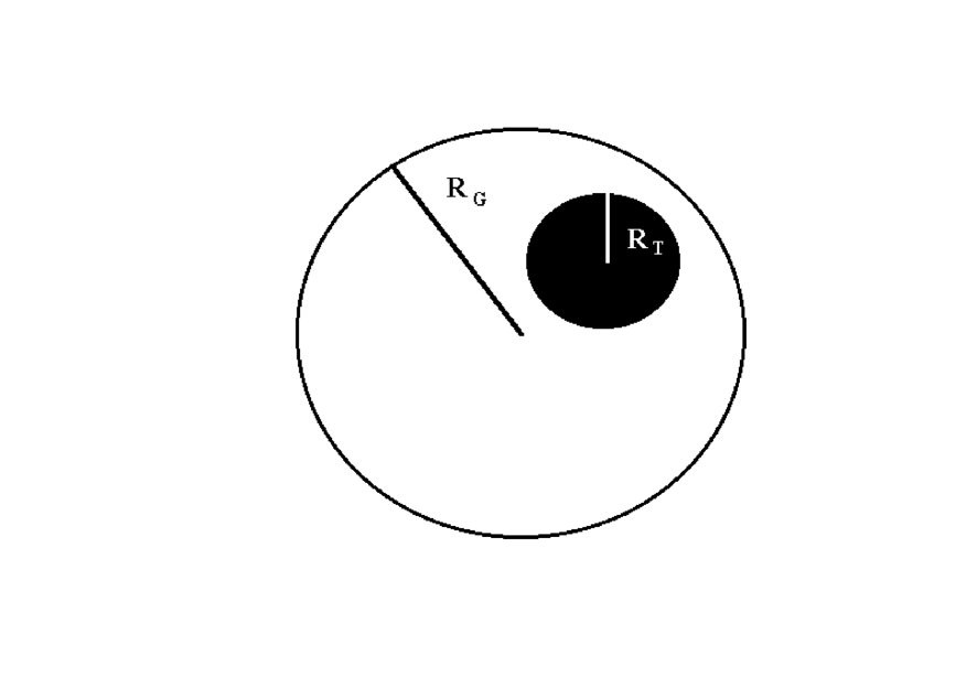
FIG. 1.:

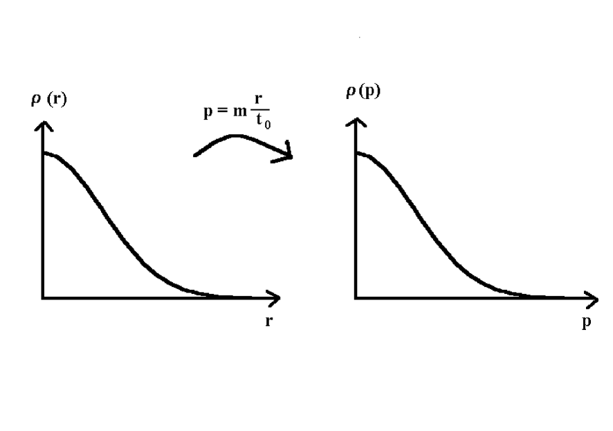
FIG. 2.:

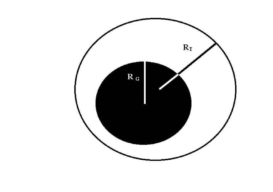
FIG. 3.:

REFERENCES

- [1] R. Hanbury-Brown and R. Q. Twiss, Phyl. Mag. 45 663 (1954); R. Hanbury-Brown and R. Q. Twiss, Nature (London) 177, (1956) 27. and 178, (1956) 1046.
- [2] T. Csörgő, ”Bose-Einstein Correlations for Longitudinally Expanding, Finite Systems”, preprint LUNFD6/(NFFL-7081) 1994, submitted for publication to Phys. Lett. B.
- [3] T. Csörgő and B. Lörstad, ”Bose-Einstein Correlations for Three-Dimensionally Expanding, Cylindrically Symmetric Finite Systems”, preprint LUNFD6/(NFFL-7082) 1994, submitted for publication to Phys. Rev. Lett.
- [4] A. Makhlin and Y. Sinyukov, Z. Phys. C39, 69 (1988).
- [5] T. Csörgő and S. Pratt, KFKI-1991-28/A, p. 75; S. Pratt, Phys. Rev. D 33, 1314 (1986).
- [6] NA35 Collaboration, Nucl. Phys. A566, (1993) 527c.
- [7] NA44 Collaboration, Nucl. Phys. A566, (1993) 115c.
- [8] M. Gyulassy, S. K. Kaufmann and L. W. Wilson, Phys. Rev. C20, (1979) 2267
- [9] W. A. Zajc in ”Particle Production in Highly Excited Matter”, H. Gutbrod and J. Rafelski eds, NATO ASI series B303 (Plenum Press, 1993) p. 435; B. Lörstad, Int. J. Mod. Phys. A12 (1989) 2861-2896.
- [10] W. Bauer, C.-K. Gelbke and S. Pratt, in Annu. Rev. Nucl. and Part. Sci., (1993)
- [11] S. Pratt, T. Csörgő and J. Zimányi, Phys. Rev. C42 1990 2646.
- [12] J. P. Bondorf, S. I. A. Garpman and J. Zimányi, Nucl. Phys. A296 (1978) 320.
- [13] G. F. Bertsch, Nucl. Phys. A498 (1989) 173c