Heavy quarkonia in the instantaneous Bethe-Salpeter model
Abstract
The heavy quarkonia (Charmonium and Bottomonium ) are investigated in the framework of the instantaneous BS-equation (Salpeter equation). We parametrize confinement alternatively by a linearly rising scalar or a vector interaction kernel and take into account the one-gluon-exchange (OGE) interaction in the instantaneous approximation. Mass spectra as well as leptonic, two-photon, E1 and M1 decay widths are calculated. Our results show that a reasonable description of the experimental data can be obtained with both spin structures for the confining kernel. The relativistic treatment leads to an improved description compared to nonrelativistic results for the two-photon width of the and to some extent for the E1-transition widths. However, characteristic deviations indicate that within a relativistic framework confinement is not described adequately by a potential.
I Introduction
In the past the heavy quarkonia have usually been investigated in the framework of the nonrelativistic quark model (see e.g. [1, 2] and references therein). Because of the large mass of the or quark the nonrelativistic treatment of the bound state problem is expected to be a good first approximation. However in charmonium one still finds typical velocities of (see e.g. ref.[3]), so that relativistic effects should become important especially for electroweak decay properties, as has been shown in ref.[1].
Relativistic calculations for the heavy quarkonia have been reported e.g. by Tiemeijer and Tjon [4] who compare various quasipotential approximations to the BS-equation, by Gara et.al. [5] within the framework of the reduced Salpeter equation, and by Murota [6] who uses the (full) Salpeter equation [7]. Unfortunately, these authors only give the mass spectra and do not calculate any decay widths, which should be most sensitive to relativistic effects.
In the present contribution we obtain the mass spectra as well as the leptonic, two-photon, E1 and M1 decay widths in the framework of the (full) Salpeter equation. We parametrize confinement by a linearly rising scalar or a vector interaction kernel and take into account the one-gluon-exchange (OGE) interaction in the instantaneous approximation. The Salpeter equation is then solved numerically according to the treatment outlined in ref.[8]. The calculation of the decay widths is performed in the Mandelstam formalism [9].
II The Model
A The Bethe-Salpeter kernel
For an instantaneous BS-kernel and free propagators with effective quark masses and one can perform the integrals in the BS-equation in the rest frame of the bound state with mass and thus arrives at the (full) Salpeter equation
| (1) | |||||
| (2) |
with and the projection operators on positive and negative energies, where is the standard Dirac hamiltonian (for the notation we refer to refs.[8, 10]).
The confinement plus OGE interaction kernel applied in the present work reads
| (3) |
where the scalar or vector confining part is given by
| (4) | |||||
| (5) |
respectively. Here is a scalar function with the fourier transform .
For the OGE kernel we have to note that it is not possible to formulate this term in a gauge-invariant way, since for a gauge-invariant kernel it is essential to take into account crossed gluon diagrams. However, for such diagrams the instantaneous approximation cannot be applied in a straightforward way. Furthermore, also in a noninstantaneous treatment the incorporation of crossed diagrams is technically very difficult, so that it would be very hard to go beyond the gauge-dependent ladder approximation.
In view of the instantaneous treatment of the OGE the natural gauge for the gluon propagator is the Coulomb gauge, which will be applied in the following. The advantage of this gauge is the fact that the gluon propagator given by
| (6) |
with is already instantaneous in its component . In the instantaneous approximation we substitute by . The OGE kernel then reads [4, 6]
| (7) |
with
| (8) |
We don’t specify the operator explicitely in momentum space since the corresponding matrix elements are evaluated in coordinate space. In analogy to the treatment of the confinement matrix elements in ref.[10] also the matrix elements of are evaluated in coordinate space. For the numerical calculation we will therefore obtain an analytic expression for the Fourier transformed OGE potential in the following.
In QCD the running coupling constant for is given by [11]
| (9) |
with
| (10) |
where in the instantaneous approximation we set . We will assume that behaves like for and reaches a saturation value for with some smooth interpolation in between.
The Fourier transformation of the OGE kernel can now be performed analytically in the short and long distance region. For only small are important in the Fourier integral and we can set so that
| (11) |
Analogously for we set and obtain (see Appendix A)
| (12) | |||||
| (14) | |||||
where is the Euler-Mascheroni constant. An interpolation between these two limiting cases is given by
| (15) |
(see ref.[4] for the case ), where we set and in order to obtain a smooth behaviour for intermediate .
The Salpeter equation with is well defined. This is in contrast to the corresponding Schrödinger equation where the terms of order like the spin-spin and spin-orbit interaction lead to a collaps of the wavefunction into the origin, i.e. the Fermi-Breit hamiltonian is unbound from below. This defect is usually cured by using first order perturbation theory or by regularizing the potential for small .
For the Salpeter equation this problem disappears due to the relativistic treatment of the quark motion. However, most Salpeter amplitudes are divergent for , as has been shown explicitely by Murota [6] for a fixed coupling constant. For a running coupling constant this divergence is less pronounced, but still present. The amplitudes are normalizable, but problems occur for decay observables like the leptonic decay widths, which depend on the value of the amplitudes at . The easiest way to cure these divergencies is to regularize the OGE kernel for small . We therefore will use the regularized potential
| (16) | |||||
| (17) |
with and determined by the condition that and its first derivative are continuous functions. The dependence of on and given by eq.(15) is not strong and can be compensated for by modifying and . We will use and for our calculation. A plot of is shown in Fig.1. The dependence of the mass spectra on the regularization parameter is very weak so that the differences in the mass spectra calculated with the regularized and unregularized potential are quite small. For our further calculation we will take .
B Calculation of decay widths
The general prescription for the calculation of any current matrix element between bound states has been given by Mandelstam [9], see e.g. [12] for a textbook treatment. The explicit formulas for the leptonic and two-photon decay widths are given in ref.[8]. Since these transitions involve a non-hadronic final state they can be calculated in the rest frame of the bound state where also the amplitudes are determined. The calculation of E1 and M1 transitions, however, involves a boost of at least one of the meson amplitudes. A covariant formulation of the Salpeter equation [13] enables to treat this boost correctly, i.e. we make the ansatz that the BS-kernel can be written covariantly as where , together with an analogous reformulation for the spin structure of . Explicitely eq.(7) can be rewritten in a covariant form by replacing (and the same for ), and .
Since the details for the calculation of electromagnetic transitions within the present framework have already been given in detail in ref.[14], we will only review the basic steps in the following.
From the Bethe-Salpeter equation
| (18) |
with , and one finds that the amputated BS amplitude or vertex function may be computed in the rest frame from the equal time amplitude as
| (19) |
Because of the covariant ansatz of the interaction kernel the kinematical boost with gives the solution of the equation for any momentum of the bound state, i.e.
| (20) |
(and analogously). The electromagnetic current between two bound states may now be calculated from the BS amplitudes and a kernel which is irreducible with respect to the incoming and outgoing quark antiquark pair, i.e. it includes all diagrams that may not be divided by just cutting the quark and the antiquark line. In lowest order the matrix element of the electromagnetic quark current taken between bound states with momenta and as shown in Fig. 2 reads explicitely
| (21) | |||||
| (22) | |||||
where is the charge of the quark and the momentum of the photon. As in the BS-equation we will use . The calculation of the current is performed in the rest frame of the incoming particle, i.e. , the results however are independent of this choice because of the formal covariance. The integral picks up only the residues of the one particle poles, the dependence is trivial for decays in z-direction and the resulting twodimensional integral in and is calculated by Gaussian integration, compare [14] for the details.
The electromagnetic decay width follows from the well known formula for the decay rate with the momentum, the polarization and the polarization vector of the photon, i.e.
| (23) | |||||
| (24) | |||||
III Results and discussion
A The model parameters
We investigate two different models of the confinement kernel: 1) a scalar - and 2) a vector -structure.
The parameters used are the charm and bottom quark masses and , the offset and slope of the confinement interaction and the saturation value for in eq.(15). These five parameters have been adjusted to the mass spectra by minimizing a that incorporates all known charmonium and bottomonium ground states and first excited states. The resulting parameter sets are given in Tab.I for the scalar (S) and the vector (V) confinement.
The main difference between the two parameter sets is given by the larger value of for the scalar confinement. This can be easily understood from the nonrelativistic picture where the spin-orbit force coming from the scalar confinement counteracts the OGE spin-orbit force, whereas for the vector confinement both spin-orbit forces affect the mass spectra in the same way. Therefore, in order to compensate the reduced spin-orbit splitting of the -states in the scalar confining case, the strength of the OGE interaction has to be increased. Compared to nonrelativistic calculations [1] we find smaller quark masses and .
It is remarkable that the slope of the confining potential comes out much larger than in nonrelativistic models, where a typical value is MeV/fm [1]. This is mainly due to the fact that in nonrelativistic calculations the kinetic energy given by is overestimated. In semirelativistic models based on the relativistic expression (see e.g. refs.[15, 16]) already higher values MeV/fm have to be used to compensate for the smaller kinetic energy. Similar values for have also been found by Gara and coworkers within the reduced Salpeter approach [5]. The admixture of the negative energy components within our full Salpeter approach leads to a further enlargement for .
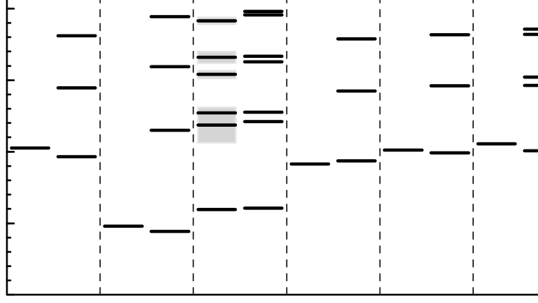
B Mass spectra
The mass spectra of Charmonium are given in Figs.3,4, the mass spectra of Bottomonium are shown in Figs.5,6 for both confinement spin structures. The experimental data are usually taken from the Particle Data Group [11]. For the recent measurement of the mass of the charmonium state () in annihilations by the E760 collaboration at Fermilab see ref.[17]. We find that both confinement spin structures give a reasonable overall description of the experimental mass spectra. The spin-spin and spin-orbit splittings are slightly better described for the vector confinement, whereas the radial excitations of the vector mesons are slightly better for the scalar confinement. However, we feel that these differences are not significant enough to decide wether the Lorentz nature of confinement should be of the scalar or vector type. This is in contrast to the nonrelativistic quark model where a scalar confinement gives the better results.
Although the description of the mass spectra can be considered quite satisfactory, there remain some characteristic deviations:
- i)
-
We find that the binding of the meson tends to be quite large. As a consequence it is not possible for a scalar confinement to obtain a satisfying simultaneous description of the hyperfine splitting and the fine splitting . The problem is less prominent for the vector confinement due to the smaller value of (see Fig.7).
- ii)
-
The large value of the confinement slope leads to an overestimation for the level spacing between the s-wave states of the vector mesons, whereas the mass differences of s-waves and d-waves is underestimated, especially for higher radial excitations.
To estimate the influence of the gauge chosen for the gluon propagator we also investigated the Feynman gauge given by
| (25) |
As shown in Fig.7 the binding energy of the meson is overestimated for this gauge. It turns out that it is not possible to compensate for this effect in a satisfying way by readjusting the model parameters. The effect of the gauge on the other states is less important.
It should be noted that due to the large quark masses the RPA-instability of the Salpeter equation with a scalar confinement as discussed in refs. [10, 18] is invisible here for any accessible number of basis states. A reasonably small number of basis states (eleven states have been used in our calculation) thus serves as a regularization supressing the very high momenta which lead to the mentioned instability. We therefore think that it is legitimate to compare the (quasistable) solutions to the experimental meson masses. Note that for light quarks, however, the instability spoils a reasonable description of light mesons for a scalar confinement, whereas for a -vector confinement the solutions remain stable.
C Decay observables
As shown in tables.II and III most decay widths show only small differences between both confinement spin structures. The improvement due to the relativistic treatment is seen most clearly in the two-photon decay of the and in the leptonic widths of the and (where a larger s-wave admixture, e.g. due to coupled channel effects, could improve the results).
The leptonic decay widths of the s-wave vector mesons are generally too large by a factor of for the and more for the higher radial excitations, whereas they are too small for the . We were not able to adjust the model parameters in order to find a better agreement with the experimental widths, since an increased leptonic width of the is usually connected with an increased width. Furthermore the leptonic widths turn out to be quite insensitive to changes of the parameters which still allow for a reasonable description of the mass spectra. The incorporation of the commonly used QCD correction factor [19] does obviously not improve these results, since the leptonic widths of the and the would be changed in the same way.
The leptonic widths of the radially excited states come out closer to the experimental data. However, the decay widths for higher radial excitations are too large compared to the widths of the lower excitations. This is due to the large value of the confinement slope which leads to an overestimation of the Salpeter amplitudes at for the higher excitations.
For the E1 and M1 transition widths we find some improvement compared to the nonrelativistic results for the transitions , and . However, for the other transitions the improvement due to relativistic effects is compensated by the influence of the large confinement slope on the Salpeter amplitudes. Note that transition amplitudes like are very sensitive to the position of the knot of the 2S amplitude..
D Comparision with previous results for light mesons
In two previous papers [10, 14] we have investigated the mass spectra, decay widths and electromagnetic form factors of light mesons within an analogous approach. For the description of the heavy quarkonia we have replaced the instanton-induced residual interaction (’t Hooft interaction) applied for the light mesons by the OGE interaction. There are two reasons which lead to this different treatment for light and heavy mesons:
- i)
-
The similarity of the charmonium and bottomonium mass spectra and the mass spectrum of positronium indicates that the OGE is a reasonable first approximation of the short-distance interaction between heavy quarks. For light quarks, however, the OGE leads to degenerate and masses in clear contradiction with experiment, whereas the ’t Hooft interaction naturally solves this problem and leads to flavormixing for the and mesons.
- ii)
-
The ’t Hooft interaction does not give first order contributions to the interaction between two charmed or bottom quarks because of the flavor antisymmetry of this interaction. Effects can only occur via flavor mixing in second order, but the large differences in the meson masses suppress such contributions. Furthermore there are no experimental indications for other flavors contributing significantly to and mesons.
We found that also for the light mesons a large value of MeV/fm (model V2 in ref.[10]) had been necessary to describe higher radial excitations and higher angular momenta . On the other hand ignoring higher radial excitations and angular momenta (model V1 in the same reference) enabled a very good description of the light pseudoscalar and vector meson ground states (i.e. , , , etc.) including various decay widths and form factors (see also ref.[14]). In this fit a much smaller value of MeV/fm had to be used which is comparable to typical values in nonrelativistic calculations.
IV Summary and conclusion
We investigated the heavy quarkonia in the framework of the Salpeter equation with a linear scalar or vector confinement plus the one-gluon-exchange interaction. For the mass spectra and the decay widths we obtained a reasonable overall agreement with the experimental meson masses for a scalar as well as for a vector confining kernel. This is in contrast to the nonrelativistic quark model where a scalar confinement is prefered.
The relativistic framework leads to an improved description especially for the two-photon decay of the and the leptonic decays of the and . Minor improvements are also found for most E1 transitions. For the other decay widths the influence of relativistic effects is compensated by the effect of the large value of the confinement slope . As a consequence the masses of the higher radial excitations and the leptonic decays cannot be described in a satisfying way.
We find that relativistic effects can be important, especially for the description of certain decays. One would expect that the covariant formulation applied in the present work should yield a systematic improvement compared to nonrelativistic calculations. However, our results for the heavy quarkonia indicate that this is not the case, which we blame on the fact that the description of confinement via a potential is not an adequate concept within a relativistic treatment.
We conclude that despite some success for certain decay widths the Salpeter approach does not allow for a satisfying description of higher radial excitations and higher angular momenta.
A The OGE potential for small distances
In this section we will analytically perform the Fourier transformation of the OGE kernel into coordinate space for as given by
| (A1) | |||||
| (A2) |
The cutoff has been introduced to keep the variable in the high momentum range where the QCD formula for the running coupling constant is approximately valid. The other cutoff has been introduced for formal reasons as shown below. It is chosen according to the condition . We basically follow the way outlined by Lucha et.al. [2] who treated the first order case, i.e. . Using and we can write
| (A3) |
with and . Rewrite
| (A4) |
Since and we have so that
| (A5) |
For the -term we further use
| (A6) |
so that we can write
| (A7) | |||||
| (A8) |
It is a good approximation to neglect terms in the following, so that
| (A9) | |||||
| (A10) |
In the limit one has , so that the limits and can be performed. With the integrals
| (A11) |
where is the Euler-Mascheroni constant and with
| (A12) |
we find
| (A13) |
The term can be neglected to a good approximation and we finally obtain eq.(14), i.e.
| (A14) | |||||
| (A16) | |||||
REFERENCES
- [1] M.Beyer, U.Bohn, M.G.Huber, B.C.Metsch, J.Resag: Z.Phys.C-Particles and Fields 55, 307 (1992)
- [2] W.Lucha, F.F.Schöberl, D.Gromes: Phys.Rep. 200, No.4, 127 (1991)
- [3] G.Hardekopf, J.Sucher, Phys.Rev. D33, 2035 (1986)
- [4] P.C.Tiemeijer, J.A.Tjon: Utrecht preprint THU-92/31 (1992); Utrecht preprint THU-93/12 (1993)
-
[5]
A.Gara,
B.Durand, L.Durand, L.J.Nickisch: Phys.Rev. D40, 843 (1989)
A.Gara, B.Durand, L.Durand: Phys.Rev. D42, 1651 (1990) - [6] T.Murota, Progr.Theor.Phys. 69, 181 (1983), ibid. 1498
- [7] E.E.Salpeter, Phys.Rev. 87, 328 (1952)
- [8] J.Resag, C.R.Münz, B.C.Metsch, H.R.Petry, Bonn TK-93-13, Nucl.Phys. A (in print)
- [9] S.Mandelstam, Proc. Roy. Soc. 233, 248 (1955)
- [10] C.R.Münz, J.Resag, B.C.Metsch, H.R.Petry, Bonn TK-93-14, Nucl.Phys. A (in print)
- [11] Particle Data Group, Phys.Rev. D45 Part II (1992)
- [12] D.Lurie: Particles and Fields, (Interscience Publishers, New York 1968)
- [13] S.J.Wallace, V.B.Mandelzweig, Nucl.Phys. A503, 673(1989)
- [14] C.R.Münz, J.Resag, B.C.Metsch, H.R.Petry, Bonn TK-94-08, bulletin board nucl-th/9406035, submitted to Phys.Rev. C
- [15] S.Godfrey, N.Isgur, Phys.Rev. D32, 189 (1985)
- [16] S.N.Gupta, S.F.Radford, W.W.Repko, Phys.Rev. D31, 160 (1985)
- [17] T.A.Armstrong et.al., Phys.Rev.Lett. 69, 2337 (1992)
- [18] J.Parramore, J.Piekarewicz, preprint of the Florida State University 1994, FSU-SCRI-94-15, bulletin board nucl-th/9402019
- [19] R.Barbieri, R.Gatto, R.Kögerler, Z.Kunszt, Phys.Lett. 57B, 455 (1975)


| Parameter | scalar | vector |
|---|---|---|
| [MeV] | 1507 | 1631 |
| [MeV] | 4857 | 5005 |
| [MeV] | -252 | -640 |
| [MeV/fm] | 1270 | 1291 |
| 0.492 | 0.365 |
| decay | experimental [11] | S | V | NR |
|---|---|---|---|---|
| 5.36 0.29 | 8.05 | 9.21 | 12.2 | |
| 2.14 0.21 | 4.30 | 5.87 | 4.63 | |
| 0.26 0.04 | 0.13 | 0.09 | 0.005 | |
| 0.75 0.15 | 3.05 | 4.81 | 3.20 | |
| 0.77 0.23 | 0.23 | 0.14 | 0.01 | |
| 0.47 0.10 | 2.16 | 3.95 | 2.41 | |
| 1.34 0.04 | 0.80 | 0.84 | 1.49 | |
| 0.59 0.03 | 0.54 | 0.57 | 0.61 | |
| 0.44 0.03 | 0.44 | 0.47 | 0.39 | |
| 0.24 0.05 | 0.40 | 0.49 | 0.33 | |
| 6.6 2.4 | 4.2 | 3.8 | 19.1 |
| decay | experimental [11] | S | V | NR |
| 22.6 4.5 | 31 | 32 | 19.4 | |
| 21.1 4.2 | 36 | 48 | 34.8 | |
| 19.0 4.0 | 60 | 35 | 29.3 | |
| 92 40 | 140 | 119 | 147 | |
| 240 40 | 250 | 230 | 287 | |
| 267 33 | 270 | 347 | 393 | |
| 1.2 0.4 | 1.4 | 1.5 | 1.00 | |
| 2.9 0.7 | 3.2 | 3.50 | 2.11 | |
| 3.1 0.8 | 3.9 | 4 | 2.59 | |
| 1.9 0.6 | 1.5 | 1.31 | 0.85 | |
| 2.9 0.7 | 2.9 | 2.88 | 1.64 | |
| 2.9 0.7 | 3.8 | 3.40 | 2.00 | |
| 13.5 | 13.0 | 13.8 | ||
| 16 | 15.3 | 15.8 | ||
| 16.5 | * | 16.8 | ||
| 1.45 | 0.95 | 2.52 | ||
| 2.32 | 2.0 | 6.15 | ||
| 3.55 | 3.0 | 10.5 | ||
| 23.2 | 21.5 | 26.2 | ||
| 26.7 | 25.5 | 30.4 | ||
| 30.0 | 30.0 | 34.6 | ||
| 0.7 0.2 | 6 | 1.3 | 4.47 | |
| 0.9 0.3 | 3.35 | 2.66 | 1.21 |