UNIVERSITY of PENNSYLVANIA
Department of Physics
David Rittenhouse Laboratory
Philadelphia PA 19104–6396

PREPRINT UPR–0087NT
July 1993

Calculation of the properties of the rotational bands of ${}^{155,157}\,$Gd

Pavlos Protopapas, Abraham Klein, and Niels R. Walet

Submitted to Physical Review C

Abstract

We reexamine the long-standing problem of the microscopic derivation of a particle-core coupling model. We base our research on the Klein-Kerman approach, as amended by Dönau and Frauendorf. We describe the formalism to calculate energy spectra and transition strengths in some detail. We apply our formalism to the rotational nuclei ^155,157Gd, where recent experimental data requires an explanation. We find no clear evidence of a need for Coriolis attenuation.

1 Introduction

In this paper we use the Kerman-Klein method [1, 2, 3] to derive a microscopic core-particle model. This method is based on Heisenberg matrix mechanics, where exact eigenstates are used, but the matrix elements of operators are the unknown quantities. In principle the formalism gives the same results as the Schrödinger equation. In practical approximations the method leads to interesting approximate models. Especially when some matrix elements are known experimentally, we can construct models that are a hybrid between a phenomenological and microscopic model. In the case of core-particle coupling such an approach has been introduced by Dönau and Frauendorf. We study the usefulness of this approach in a serious numerical application to the rotational nuclei ^155,157Gd, and extend the method to calculations of transition strengths.

Our calculations, restricted to deformed nuclei in the current application, generalize the particle rotor model, and we shall compare our results to those of less microscopic calculations using this model. The model, first introduced by Bohr and Mottelson [4], has been used for the study of both low and high spin states of weakly and strongly deformed nuclei. For the past three decades it has continued to provide a framework for the analysis of the rotational band structure of odd nuclei. In spite of its approximate nature, it has been used successfully to explain both the structure of deformed and transitional nuclei [5].

In its most primitive version one couples a single particle to a rotating (even-even) rigidly deformed core. The coupling of the single particle to the core is generally approximated by a deformed Nilsson potential. Due to the rotation there is also a Coriolis interaction between the total angular momentum of the system and the single-particle angular momentum. In later applications one finds extensions of the original model (we shall use calculations for ^155,157Gd as references throughout the discussion). The Nilsson potential can be replaced by a more realistic deformed Woods-Saxon potential [6], pair correlations can be taken into account by a quasi-particle transformation of BCS type [6, 7, 8, 9], and mixing between different major shells (states with principal quantum number $N$ differing by two) [10, 11, 12, 13, 8, 9] can be included. Finally one can allow for phonon excitations of the core [6, 7, 14, 15], in contrast with the standard core-particle coupling model (CPC model) where the core is assumed to be a rigid rotor.

Even these extended models often suffer from an inadequacy, the so called Coriolis attenuation problem. In order to reproduce the experimental energy spectra, the Coriolis matrix elements have to be reduced by up to $50\%$. This problem has been studied extensively over the years. Many physical effects previously omitted in the model have been invoked as the cure for this disease: the proper treatment of the two body recoil effect [16], the inclusion of octupole degrees of freedom [17], and the use of an angular-momentum dependent moment of inertia and pairing gap [18]. A more complete list of all possible suggested causes is given in Ref. [19]. It is quite conceivable that one needs to combine several of these extensions to eliminate this problem. As yet, however, no clear consensus has emerged concerning the source of the attenuation problem.

In the present paper we adopt the Kerman-Klein approach, emphasizing the steps required in the transition between a strict microscopic approach and one which contains compromises aimed at making applications easier to carry out. In effect we shall trace the steps of Dönau and Frauendorf in their core-quasiparticle coupling model [5, 20, 21]. In their work a simple pairing and quadrupole-quadrupole separable interaction Hamiltonian was considered. Only a few application of this type exist, see Refs. [22, 23] and the review in Ref. [19]. In our work we also introduce mixing between states with $\Delta N=\pm 2$, where $N$ is the principal quantum number. We believe that the pursuit of a microscopic approach will lead to a more complete CPC, and give some insight into the problems of phenomenological CPC models. In addition the microscopic basis allows for the straightforward inclusion of different effective interactions.

This paper is organized as follows. In Sec. 2, we discuss the basis of the model. First we describe briefly the basis of the Kerman-Klein method and then summarize the Dönau-Frauendorf modifications [5, 20, 21]. We then turn to the application of a slightly extended form of the Dönau-Frauendorf formulation to the nuclei ^155,157Gd. These form an excellent testing ground for our model since extensive calculations have been performed for these nuclei. There also exists a body of recent experimental data on the transition strengths that has not yet been explored sufficiently [24]. Finally, in the last section, we give a review of the other theoretical descriptions available for these nuclei, and compare our results with these previous efforts.

2 The Model

2.1 Kerman-Klein Method

The Kerman-Klein method was introduced in the early sixties [25] to provide a rotationally invariant description of deformed nuclei in the framework based on the equations of motion (EOM). Among many applications, it was applied to a study of the foundations of core-particle coupling models [1, 26]. Overall it has been applied to various nuclear many-body problems [2] as well as to field theories [27, 28]. Here we use it as the starting point to derive and extend the CPC model. As has been stated in the introduction, one of the major difficulties with the CPC model is the Coriolis attenuation problem. We believe that the Kerman-Klein method may be a good starting point for an investigation of this problem. The method starts from a shell model Hamiltonian and provides expressions for the properties of low-lying collective states of an odd-mass nucleus and its even-even neighbors. These expressions include the energy eigenvalues, the single-particle coefficients of fractional parentage (cfp) and matrix elements of the electromagnetic operators. In practice, Hamiltonians with only simple ingredients have been studied (in the simplest case single particle Hamiltonian plus monopole pairing and quadrupole-quadrupole interactions), and only relatively few low-lying collective states in the even cores have been included (in the simplest case only the ground-state rotational band). Since the Hamiltonian must include expressions for both the long-range part and the short-range part of the nuclear force, we start with a Hamiltonian containing multipole expansions involving particle-hole as well as particle-particle contributions. This separation simplifies the application of the EOM method.

We thus write

$$H=\sum_{a}h_{a}a^{{\dagger}}_{\alpha}a_{\alpha} + \frac{1}{8}\sum_{abcd}\sum_{LM_{L}}{F_{acdb}(L)}\,{B^{{\dagger}}_{LM_{L}}(a,c)}{B_{LM_{L}}(d,b)}$$ (1)

$$+ \frac{1}{8}\sum_{abcd}\sum_{LM_{L}}G_{abcd}(L)\,A^{{\dagger}}_{LM_{L}}(a,b)A_{LM_{L}}(c,d).$$

Here $h_{a}$ ($\alpha=(j_{a},m_{a})$ and $a=j_{a}$) are the spherical single particle energies, the operator $B_{LM}$ is the particle-hole multipole operator,

$$B^{{\dagger}}_{LM_{L}}(a,b)\equiv\sum_{m_{a}m_{b}}s_{\beta}\;{C^{LM_{L}}_{\alpha\bar{\beta}}}\;{a^{{\dagger}}_{\alpha}}{a_{\beta}}=\left[a_{a}^{{\dagger}}\times\tilde{a}_{b}\right]_{M_{L}}^{L},$$ (2)

and $A_{LM}$ is the particle-particle multipole operator

$$A^{{\dagger}}_{LM_{L}}(a,b)\equiv\sum_{m_{a}m_{b}}C^{LM_{L}}_{\alpha\beta}\;{a^{{\dagger}}_{\alpha}}{a^{{\dagger}}_{\beta}}=\left[a_{a}^{{\dagger}}\times a_{b}^{{\dagger}}\right]_{M_{L}}^{L},$$ (3)

where $C_{\alpha\beta}^{LM}$ are the Clebsch-Gordan coefficients and $s_{\alpha}=(-)^{j_{a}-m_{a}}$. The coefficients $F$ are the particle-hole matrix elements

$${F_{acdb}(L)}\equiv 2\sum_{m^{\prime}s}{s_{\gamma}}{s_{\beta}}\;{C^{LM_{L}}_{\alpha\bar{\gamma}}}\,{C^{LM_{L}}_{\delta\bar{\beta}}}\,\,V_{\alpha\beta\gamma\delta},$$ (4)

and $G$ the particle-particle matrix elements

$$G_{abcd}(L)\equiv 2\sum_{m^{\prime}s}{C^{LM_{L}}_{\alpha\beta}}\,{C^{LM_{L}}_{\gamma\delta}}\,V_{\alpha\beta\gamma\delta}{}.$$ (5)

The task we set ourselves is to obtain equations for the states and energies of the odd nucleus assuming that the properties of the even nuclei are known. The states of the odd nucleus (particle number $N$) are designated as $\left|\nu\,J\mu\right>$ where $\nu$ denotes all quantum numbers beside the angular momentum $J$ and its projection $\mu$. The eigenstates and eigenvalues of the neighboring even nuclei with particle numbers ($N\pm 1$) are $\left|IM\,n\,(N\pm 1)\right>$ and $E_{In}^{N\pm 1}$, respectively, where $n$ plays the same role for even nuclei as $\nu$ does for the odd nuclei. The equations of motion (EOM) are obtained by forming commutators between the Hamiltonian and single fermion operators,

$$\left[a_{\alpha},H\right]=h_{a}a_{a} + \frac{1}{4}\sum_{bd\gamma}\sum_{LM}C_{\alpha\gamma}^{LM}G_{acbd}(L)a^{{\dagger}}_{\gamma}A_{LM}(c,d)$$ (6)

$$+ \frac{1}{4}\sum_{bd\gamma}\sum_{LM}{s_{\gamma}}C_{\alpha\bar{\gamma}}^{LM}F_{acdb}(L)a_{\gamma}B_{LM}(d,b),$$

$$\left[a^{{\dagger}}_{\alpha},H\right]=-h_{a}a_{a}^{{\dagger}} - \frac{1}{4}\sum_{bd\gamma}\sum_{LM}C_{\alpha\gamma}^{LM}G_{acbd}(L)A^{{\dagger}}_{LM}(c,d)a_{\gamma}$$ (7)

$$- \frac{1}{4}\sum_{bd\gamma}\sum_{LM}{s_{\gamma}}C_{\alpha\bar{\gamma}}^{LM}F_{acdb}(L)B^{{\dagger}}_{LM}(d,b)a^{{\dagger}}_{\gamma}.$$

The matrix elements of these equations provide expressions for the single particle coefficients of fractional parentage $U$ and $V$, defined as

$$U^{\nu}_{J\mu}(\alpha;IMn)=\left<\nu J\mu\mid a_{\bar{\alpha}}^{{\dagger}}\mid IMn(N-1)\right>,$$ (8)

$$V^{\nu}_{J\mu}(\alpha;IMn)=\left<\nu J\mu\mid a_{\alpha}\mid IMn(N+1)\right>{}.$$ (9)

These are obtained by the evaluation of matrix elements of the EOM (6,7) between eigenstates $\left|\nu J\mu\right>$ and $\left|IMn(N\pm 1)\right>$ and the use of the completeness relation (details of the derivation can be found in [25]). The resulting equations can be cast into the block matrix form,

$$\left(\begin{array}[]{cc}\epsilon+\omega^{N+1}+\Gamma^{N+1}&\Delta^{N+1}\\ &\\ \Delta^{{\dagger}N-1}&-\epsilon+\omega^{N-1}-\Gamma^{{\dagger}N-1}\end{array}\right)\left(\begin{array}[]{c}U\\ \\ V\end{array}\right)={\cal E}_{\nu J}\left(\begin{array}[]{c}U\\ \\ V\end{array}\right).$$ (10)

Here $\epsilon$ are the single particle energies measured relative to the chemical potential, $\lambda$, the elements of $\omega$ are the excitation energies in the even nuclei, and $\Gamma$ and $\Delta$ are pair and multipole fields. More specifically we have

$$\epsilon_{\alpha IMn,\gamma I^{\prime}M^{\prime}n^{\prime}} = (\lambda_{N}-h_{a})\delta_{\alpha\gamma}\delta_{II^{\prime}}\delta_{MM^{\prime}}\delta_{nn^{\prime}},$$ (11)

$$\lambda_{N} = \frac{1}{2}\left[E_{0}^{N+1}-E_{0}^{N-1}\right],$$ (12)

$$\omega^{N\pm 1}_{\alpha IMn,\gamma I^{\prime}M^{\prime}n^{\prime}} = (E_{In}^{N\pm 1}-E_{0}^{N\pm 1})\delta_{\alpha\gamma}\delta_{II^{\prime}}\delta_{MM^{\prime}}\delta_{nn^{\prime}},$$ (13)

$$\Gamma^{N\pm 1}_{\alpha IMn,\gamma I^{\prime}M^{\prime}n^{\prime}}=\sum_{LM_{L}}\sum_{bd}{s_{\gamma}}C_{\alpha\bar{\gamma}}^{LM_{L}}F_{acdb}(L)\hskip 142.26378pt$$

$$\times\left<I^{\prime}M^{\prime}n^{\prime}(N\pm 1)\mid B_{LM_{L}}(d,b)\mid IMn(N\pm 1)\right>,$$ (14)

$$\Delta^{N\pm 1}_{\alpha IMn,\gamma I^{\prime}M^{\prime}n}=\sum_{LM_{L}}\sum_{bd}C_{\alpha\gamma}^{LM_{L}}G_{acdb}(L)\hskip 142.26378pt$$

$$\times\left<I^{\prime}M^{\prime}n^{\prime}(N-1)\mid A_{LM_{L}}(d,b)\mid IMn(N+1)\right>.$$ (15)

In order to specify the solutions uniquely a normalization condition is required. From the anti-commutation relations of the fermion operators, one takes the appropriate matrix elements using a sum over intermediate states and finds

$$\frac{1}{\Omega}\sum_{\alpha\,IMn}\left[|U^{\nu}_{J\mu}(\alpha IM;n)|^{2}+|V^{\nu}_{J\mu}(\alpha IM;n)|^{2}\right]=1,$$ (16)

where

$$\Omega=\sum_{j_{a}}(2j_{a}+1).$$ (17)

All of the above equations are still exact and represent a formulation of Heisenberg’s matrix mechanics. The fundamental practical problem is to find a suitable ‘collective’ subspace of the complete Hilbert space. We assume that this ‘collective’ subspace decouples from the remaining states, at least approximately. This requires that any matrix element of the relevant multipole operators between a collective and a non-collective state is negligible.

2.2 The Dönau-Frauendorf Model

In this section we introduce the approximations made by Dönau and Frauendorf, and use these as the practical basis for our investigation. First we assume that we have a finite sum of separable interactions, where each of the terms in (4) and (5) is of the form

$$F_{acdb}(L)=-2\kappa_{L}F_{ac}(L)F_{db}(L),$$ (18)

$$G_{acdb}(L)=-2g_{L}G_{ac}(L)G_{db}(L).$$ (19)

Here $\kappa_{L}$, $g_{L}$ are the strengths of the corresponding multipole and pairing forces, and $F_{ac}(L)$ and $G_{ac}(L)$ are the appropriate single particle matrix elements. For the moment we consider only monopole-pairing and quadrupole-quadrupole interaction (the inclusion of hexadecapole and the quadrupole-pairing interactions is left for later work). The quadrupole-quadrupole and monopole-pairing operators are

$$Q_{M}=\sum_{ac}F_{ac}(2)B_{2M}(a,c),$$ (20)

$$\Delta=\sum_{ac}G_{ac}(0)A_{00}(a,c).$$ (21)

co-workers have adopted Next we identify the “collective” subspace appropriate for the applications that follow. The obvious choice is the ground state rotational band $\left|IMK=0\right>$, where $K$ is the projection of angular momentum on the body fixed axis. The fact that this “collective” subspace approximately decouples from the remaining states is equivalent to the requirement that inter-band $BE(2)$ transitions are much smaller than the intra-band transitions. This is generally true for deformed nuclei. A last approximation for deformed nuclei, convenient but not necessary, is to replace the excitation energies as well as the multipole and pairing fields by their average values for the two neighboring even-even nuclei.

Before we go on to the next step it is convenient to rewrite the EOM with reduced matrix elements, using the Wigner-Eckart theorem. We can thus derive equations of motion, again dropping all indices,

$$\left(\begin{array}[]{cc}\epsilon+\omega+\Gamma&\Delta\\ &\\ \Delta&-\epsilon+\omega-\Gamma\end{array}\right)\left(\begin{array}[]{c}V\\ \\ U\end{array}\right)={\cal E}_{\nu J}\left(\begin{array}[]{c}V\\ \\ U\end{array}\right),$$ (22)

where $V$ and $U$ are the reduced cfp

$${U_{J}^{\lambda}(1;I)}{a} \equiv \left<\nu J\parallel a^{{\dagger}}_{a}\parallel I(N-1)\right>,$$

$${V_{J}^{\lambda}(1;I)}{a} \equiv \left<\nu J\parallel\tilde{a}_{a}\parallel I(N+1)\right>,$$ (23)

the self-consistent fields are represented by the expressions

$$\Gamma_{aI,cI^{\prime}}=-\frac{1}{2}\kappa_{2}(-)^{J_{c}+I+J}{\left\{\begin{array}[]{ccc}{\scriptstyle j_{a}}&{\scriptstyle{j_{c}}}&{\scriptstyle 2}\\ {\scriptstyle I^{\prime}}&{\scriptstyle I}&{\scriptstyle J}\end{array}\right\}}\left<I\parallel Q_{2}\parallel I^{\prime}\right>F_{ac}(2),$$ (24)

and the generalized pairing force is approximated by a constant gap energy for all levels,

$$\Delta_{aI,cI^{\prime}}=\left<I\|\Delta\|I^{\prime}\right>\delta_{ac}\approx\left<0\|\Delta\|0\right>\delta_{II^{\prime}}\delta_{ac}{}.$$ (25)

The normalization condition becomes

$$\frac{1}{\Omega}\sum_{a\,I}\left[|{U_{J}^{\lambda}(1;I^{\prime})}{a}|^{2}+|{V_{J}^{\lambda}(1;I^{\prime})}{a}|^{2}\right]=1.$$ (26)

Here the inclusion of only the collective subspace is somewhat more questionable than for the EOM, but there appears to be no simple alternative.

The final step in the derivation is the replacement of the self consistent fields by phenomenological inputs. In this context $\left<I\|Q\|I^{\prime}\right>$ and $\Delta$ are the quadrupole matrix elements of the neighboring even nuclei and $\Delta$ their gap energies. The quadrupole fields can either be extracted from experiment or calculated using a phenomenological model such as the Bohr-Mottelson model [4],

$$\left<I^{\prime}\|Q\|I\right>=q_{0}\,\sqrt{\frac{5}{16\pi}}\,\sqrt{(2I+1)(2I^{\prime}+1)}\,{\left(\begin{array}[]{ccc}{\scriptstyle I}&{\scriptstyle 0}&{\scriptstyle I^{\prime}}\\ {\scriptstyle 0}&{\scriptstyle 2}&{\scriptstyle 0}\end{array}\right)},$$ (27)

where $q_{0}$ is a phenomenological input which can be obtained from experimental values.

Having described the assumptions involved in the derivation of the model, we turn to the task of solving the resulting equations. The main difficulty in solving those equations is that the set of solutions (22) is over-complete by a factor of two. This is a consequence of the fact that the basis states $a^{{\dagger}}\left|I(N-1)\right>$ and $a\left|I(N+1)\right>$ form an over-complete and non-orthogonal set as in the standard BCS model. Half of the states found by solving (22) are spurious, and these have to be identified. To remove the spurious solutions one can proceed in the following way [20, 21]: First build the density matrix

$$D_{aa^{\prime}}(II^{\prime})=\sum_{\nu J}\hskip 289.07999pt$$

$$\left[\begin{array}[]{cc}\left<I(N-1)\|a_{a}\|\nu J\right>\left<\nu J\|a^{{\dagger}}_{a^{\prime}}\|I^{\prime}(N-1)\right>&\left<I(N+1)\|a^{{\dagger}}_{a}\|\nu J\right>\left<\nu J\|a^{{\dagger}}_{a^{\prime}}\|I^{\prime}(N-1)\right>\\ \\ \left<I(N-1)\|a_{a}\|\nu J\right>\left<\nu J\|a_{a^{\prime}}\|I^{\prime}(N+1)\right>&\left<I(N+1)\|a^{{\dagger}}_{a}\|\nu J\right>\left<\nu J\|a_{a^{\prime}}\|I^{\prime}(N+1)\right>\end{array}\right],$$ (31)

which can also be expressed in terms of the reduced cfp $U$ and $V$,

$$D_{aa^{\prime}}(II^{\prime})=\sum_{J}D_{aa^{\prime}}^{J}(II^{\prime})=\sum_{J\nu}\left[\begin{array}[]{cc}{U_{J}^{\lambda}(1;I)}{\alpha}{U_{J}^{\lambda}(1;I^{\prime})}{\alpha^{\prime}}&{U_{J}^{\lambda}(1;I)}{\alpha}{V_{J}^{\lambda}(1;I^{\prime})}{\alpha^{\prime}}\\ \\ {V_{J}^{\lambda}(1;I)}{\alpha}{U_{J}^{\lambda}(1;I^{\prime})}{\alpha^{\prime}}&{V_{J}^{\lambda}(1;I)}{\alpha}{V_{J}^{\lambda}(1;I^{\prime})}{\alpha^{\prime}}\end{array}\right]{}.$$ (32)

This density matrix has two important properties; it commutes with Hamiltonian

$$\left[H,D\right]_{J}=0,$$ (33)

where $H$ is the matrix Hamiltonian of Eq. (22) and the scaled quantity $\Omega\,$D acts like a projection operator

$$(\Omega D)^{2}=\Omega D.$$ (34)

(Here (33) follows from the EOM and (34) expresses the ortho-normalization conditions that follow from (22) and (26).)

Therefore, $D$ has eigenvalues $1/\Omega$ or 0. The eigenstates of the Hamiltonian which are also eigenstates of $D$ with eigenvalue $1/\Omega$ describe the real quasiparticle excitations in the odd-$N$ nucleus, whereas the eigenstates with eigenvalue 0 characterize the spurious states.

We next decompose the Hamiltonian as,

$$H=H_{qp}+H_{c},$$ (35)

where

$$H_{qp}=\left(\begin{array}[]{cc}-\epsilon-\Gamma&\Delta\\ \Delta&\epsilon+\Gamma\end{array}\right),\hskip 28.45274ptH_{c}=\left(\begin{array}[]{cc}\omega_{c}&0\\ 0&\omega_{c}\end{array}\right){}.$$ (36)

$H_{qp}$ is interpreted as a generalized quasi-particle Hamiltonian and $H_{c}$ as the core Hamiltonian. $H$ is separated into two parts because $H_{qp}$ is antisymmetric with respect to particle-hole conjugation ($a_{a}^{{\dagger}}\rightarrow a_{a}$ ), and therefore, as in the usual BCS theory [29], the solutions of this part of the Hamiltonian are divided into two sets with sign-reversed energies; the negative energy solutions are the spurious states. This decomposition gives a good starting point for a numerical technique to remove the spurious states. First, we turn off the core Hamiltonian $H_{c}$. We solve the eigenvalue problem, $H_{qp}\Psi^{0}={\cal E}^{0}\Psi^{0}$, and find the solutions $\Psi^{0}_{\pm}$ and $\pm{\cal E}^{0}$ where

$$\Psi^{0}=\left(\begin{array}[]{c}V^{0}\\ U^{0}\end{array}\right){}.$$

From the physical states $\Psi_{+}^{0}$ we can construct the density matrix $D^{0}$ as in (32). Then the core Hamiltonian is gradually turned on,

$$H(\gamma)=H_{qp}+\gamma H_{c},$$ (37)

where $\gamma$ is a scaling parameter. The next step is to diagonalize $H(\gamma)$ and find the new solutions, $\Psi(\gamma)$. If the change of $\gamma$ is not too big, the quantity $\Psi^{{\dagger}}(\gamma)D^{0}\Psi(\gamma)$ will either be close to 0 or to $1/\Omega$. When the value of $\Psi^{{\dagger}}(\gamma)D^{0}\Psi(\gamma)$ is close to $1/\Omega$ it is a real state and when it is close to zero it is a spurious state. Now we can construct the new density matrix from the physical states $\Psi_{+}(\gamma)$ which we call $D^{1}$. Then $\gamma$ is incrementally increased and this process is repeated until $\gamma=1$. In practice this method works very well since the change in the eigenvalues of $D$ never exceeds $5\%$, even with only 15 incremental steps.

When $\gamma\rightarrow 0$, which is the limit that the moment of inertia ${\cal I}$ goes to infinity, the core excitations vanish (adiabatic limit). In this limit, $H_{qp}$ is equivalent to the usual Nilsson plus pairing Hamiltonian. To demonstrate this, we first diagonalize the particle-hole part ($\epsilon+\Gamma$) of $H_{qp}$. The resulting eigenvalues $e_{k}-\lambda$ are characterized by the index $k$. For each different $k$, $\Gamma$ defines a different fixed quadrupole field or, in other words, an instantaneous orientation of the core. The index $k$ can be related to $K$, the projection of the angular momentum on the body fixed frame, by a method described below. Finally, the solutions of the $H_{qp}$, including pairing, are

$${\cal E}^{\pm}_{K}=\pm\sqrt{(e_{k}-\lambda)^{2}+\Delta^{2}}{}.$$ (38)

The remaining problem is to find the correspondence between the values of $K$ and those of $k$. This is not straightforward because H_qp is an angular momentum conserving quantity; therefore $K$ can not be obviously associated with the eigenvalues. We use the fact that among states with different $J$, states with the same value of $K$ have identical eigenvalues. We can extract a unique state of maximal $K$ value in the following way: Compare the $J+1/2$ doubly degenerate solutions for angular momentum $J$ with the $J-1/2$ doubly degenerate solutions for $J-1$. Since the maximum values of $K$ are $J$ and $J-1$, respectively, the additional pair of solutions for angular momentum $J$ must have $|K|=J$. We then proceed with $J-2$, and so on.

2.3 Electromagnetic Transitions

The electromagnetic multipole operators are one-body matrix elements of the form

$$T_{LM}=\sum_{\alpha\gamma}^{\pi\nu}e_{\alpha\gamma}t_{\alpha\gamma}a^{{\dagger}}_{\alpha}a_{\gamma},$$ (39)

where $e_{\alpha\gamma}$ is either the effective charge or the effective $g$ factor, and $t_{\alpha\gamma}$ are the single-particle matrix elements of the transition operator.

It is convenient to decompose the electromagnetic observables into core and particle contribution, as in the conventional CPC. To do this we must express the matrix elements of the transition multipole operator of the odd nucleus, $\left<J^{\prime}\mu^{\prime}\nu^{\prime}|T_{LM}|J\mu\nu\right>$, in terms of the matrix elements of the even nuclei (which are known from experiment) and the known eigenfunctions $U$ and $V$. We use the decomposition of the eigenstates of the odd nucleus [5, 20],

$$\left|J\mu\nu\right>=\frac{1}{\Omega}\sum_{IM\alpha}\left[U_{J\mu}^{\nu}(\alpha;IM)\,a_{\alpha}^{{\dagger}}\,\left|IM\right>+V_{J\mu}^{\nu}(\alpha;IM)\,a_{\alpha}\,\left|\widetilde{IM}\right>\right],$$ (40)

where

$$\left|IM\right> = \left|IM(N-1)\right>,$$

$$\left|\widetilde{IM}\right> = \left|IM(N+1)\right>.$$ (41)

We then rearrange the order of the single particle operators $a$ and $a^{{\dagger}}$ and the collective operator $T$ using their commutation relations and utilize sums over intermediate states of the even nuclei such that operator $T$ stands between states of the even n uclei and the single particle operators occur between an even nucleus state and an odd nucleus state. Finally we have

$$\left<J^{\prime}\mu^{\prime}\nu^{\prime}|T_{Lm}|J\mu\nu\right> = \frac{1}{\Omega}\sum_{IM\alpha}\sum_{I^{\prime}M^{\prime}}\left[U_{J\mu}^{\nu}(\alpha;IM)U_{J^{\prime}\mu^{\prime}}^{\nu^{\prime}}(\alpha;I^{\prime}M^{\prime})\left<I^{\prime}M^{\prime}\mid T_{Lm}\mid\widetilde{IM}\right>\right.$$

$$\hskip 14.45377pt\left.+V_{J\mu}^{\nu}(\alpha;IM)V_{J^{\prime}\mu^{\prime}}^{\nu^{\prime}}(\alpha;I^{\prime}M^{\prime})\left<I^{\prime}M^{\prime}\mid T_{Lm}\mid\widetilde{IM}\right>\right]$$

$$+ \frac{1}{\Omega}\sum_{IM\alpha}\sum_{\gamma}e_{\alpha\gamma}t_{\alpha\gamma}\left[U_{J\mu}^{\nu}(\alpha;IM)U_{J^{\prime}\mu^{\prime}}^{\nu^{\prime}}(\gamma;IM)+V_{J\mu}^{\nu}(\alpha;IM)V_{J^{\prime}\mu^{\prime}}^{\nu^{\prime}}(\gamma;IM)\right].$$

Equation (2.3) clearly exhibits a separation into particle and core contributions. With the definition of the reduced matrix elements (23) we ultimately obtain

$$\left<J^{\prime}\nu^{\prime}\|T_{L}\|J\nu\right> = \frac{1}{\Omega}\sum_{aII^{\prime}}\left<I\|T_{L}\|I^{\prime}\right>(-)^{j_{a}+J+I^{\prime}}\,{\left\{\begin{array}[]{ccc}{\scriptstyle I^{\prime}}&{\scriptstyle I}&{\scriptstyle 2}\\ {\scriptstyle J}&{\scriptstyle J^{\prime}}&{\scriptstyle j_{a}}\end{array}\right\}}\left[U_{J}^{\nu}(a;I)U_{J^{\prime}}^{\nu^{\prime}}(a;I^{\prime})+V_{J}^{\nu}(a;I)V_{J^{\prime}}^{\nu^{\prime}}(a;I^{\prime})\right]$$ (45)

$$+ \frac{1}{\Omega}\sum_{Iac}(-)^{j_{a}+J^{\prime}+I}e_{ac}t_{ac}{\left\{\begin{array}[]{ccc}{\scriptstyle J}&{\scriptstyle J^{\prime}}&{\scriptstyle 2}\\ {\scriptstyle j_{c}}&{\scriptstyle{j_{a}}}&{\scriptstyle I}\end{array}\right\}}\left[U_{J}(a;I)U_{J^{\prime}}^{\nu^{\prime}}(c;I)+V_{J}(a;I)V_{J^{\prime}}^{\nu^{\prime}}(c;I)\right],$$ (48)

where we assume that the matrix elements of $T_{L}$ do not depend on $N$,

$$\left<I\|T_{L}\|I^{\prime}\right>=\left<\tilde{I}\|T_{L}\|\tilde{I^{\prime}}\right>{}.$$ (49)

For the electric quadrupole transitions studied in this paper, the matrix elements $\left<I\|T_{L}\|I^{\prime}\right>$ become the matrix elements of the quadrupole operator $\left<I\|Q\|I^{\prime}\right>$. The single particle matrix element $t_{ac}(L)$ are

$$F_{ac}(L)=\left<a\parallel r^{2}Y^{2}\parallel c\right>.$$ (50)

For these electric transitions we have only one parameter to fix, the effective charge. As we will see later this is a minor problem since the single particle contribution is much smaller than the core contribution. The quadrupole matrix elements of the core can be either derived from the Bohr-Mottelson model as in (27) or extracted from the experimental results.

For the magnetic ($M1$) transitions the matrix elements of the operator is

$$\left<I\|T_{L}\|I^{\prime}\right>=\left<I\|M\|I\right>\ delta_{II^{\prime}},$$ (51)

and the single particle matrix elements $t_{ac}$ become [29]

$$t_{ac}=G_{ac} = \left<j_{a}\parallel M\parallel j_{c}\right>$$ (55)

$$= \left<n_{a}l_{a}j_{a}\mid n_{c}l_{c}j_{c}\right>\sqrt{\frac{3\,(2j_{a}+1)\,(2j_{c}+1)}{4\pi}}(-1)^{j_{c}-1/2}\left(\begin{array}[]{ccc}j_{a}&1&j_{c}\\ -1/2&0&1/2\end{array}\right)$$

$$\hskip 144.54pt\times(1-k)\left[\frac{1}{2}g_{s}-g_{l}(1+\frac{k}{2})\right],$$

with

$$k=(j_{a}+\frac{1}{2})(-1)^{(j_{a}+l_{a}+1/2)}+(j_{c}+\frac{1}{2})(-1)^{(j_{c}+l_{c}+1/2)}{}.$$ (56)

3 Calculations for ^155,157Gd

We decided to concentrate the calculations on the nuclei ^155,157Gd, since recent detailed studies of the transitions [24] seem to require explanation. The even cores ^154,156,158Gd are well deformed and have almost rigid rotational bands. Therefore, the quadrupole field $\Gamma$ can be estimated using the Bohr-Mottelson model as

$$\Gamma_{aI,cI^{\prime}}=-\frac{22.21}{2}\,\kappa\beta A^{2/3}(-)^{j_{c}+I+J}{\left\{\begin{array}[]{ccc}{\scriptstyle j_{a}}&{\scriptstyle{j_{a}}}&{\scriptstyle 2}\\ {\scriptstyle I}&{\scriptstyle I^{\prime}}&{\scriptstyle J}\end{array}\right\}}\sqrt{(2I+1)(2I^{\prime}+1)}{\left(\begin{array}[]{ccc}{\scriptstyle I}&{\scriptstyle 0}&{\scriptstyle I^{\prime}}\\ {\scriptstyle 0}&{\scriptstyle 2}&{\scriptstyle 0}\end{array}\right)}q_{ac},$$ (57)

where $q_{ac}$ are the single particle quadrupole matrix elements (labeled before by $F_{ac}(2)$) in fm. The factor 22.21 comes from the transformation from the intrinsic quadrupole moment to the deformation parameter $\beta$. The core energies are $\omega_{I}=\frac{I(I+1)}{2{\cal I}}$, where for the moments of inertia the values ${\cal I}^{155}=0.0122\,$MeV , ${\cal I}^{157}=0.0124\,$MeV are chosen. For the pairing potential we used the value $\Delta=\frac{127}{A}$ MeV. The chemical potential $\lambda^{N}$ was calculated according to (12) from the difference between the ground state energies of the cores. The values found are $\lambda^{155}=-7.4845\,$MeV and $\lambda^{157}=-7.1488\,$MeV. The experimental values for the quadrupole deformations of the cores are [30]

$$\begin{array}[]{cc}{}^{154}\,\rm{Gd}:&\beta_{20}=0.3294,\\ {}^{156}\,\rm{Gd}:&\beta_{20}=0.3378,\\ {}^{158}\,\rm{Gd}:&\beta_{20}=0.3484.\end{array}$$

For the odd nuclei we used the averages of the two neighboring even nuclei, $\beta_{20}^{155}=0.329$, $\beta_{20}^{157}=0.3431$. The strength of the quadrupole force $\kappa$ was taken as a free parameter. The single particle wave functions were found from a Woods-Saxon potential [29],

$$V^{ws}(r)=\frac{-V_{0}}{1+\exp\left(\frac{r-R_{0}}{a}\right)},$$ (58)

including spin-orbit interaction with parameters $a=0.65$, $R_{0}=1.25A^{1/3}$ and $V_{0}=51/\left(1-\frac{2}{3}\frac{N_{p}-Z}{A}\right)$ MeV. The single particle quadrupole matrix elements $q_{ac}$ take values according to the standard formula [29]

$$q_{ac} = \left<j_{a}\parallel Q\parallel j_{c}\right>$$ (59)

$$= \left<n_{a}l_{a}j_{a}\mid r^{2}\mid n_{c}l_{c}j_{c}\right>\sqrt{\frac{5\,(2j_{a}+1)\,(2j_{c}+1)}{4\pi}}(-1)^{j_{c}-1/2}{\left(\begin{array}[]{ccc}{\scriptstyle j_{a}}&{\scriptstyle 2}&{\scriptstyle j_{c}}\\ {\scriptstyle-1/2}&{\scriptstyle 0}&{\scriptstyle 1/2}\end{array}\right)}{}.$$ (62)

The resulting single-particle levels are shown in Fig. 1.

Figure 1: Single particle eigenvalues for Woods-Saxon potential .

First we apply the method to positive parity states of ¹⁵⁷Gd. The experimental results identify the $5/2^{+}[642]$ band as the lowest positive parity band, followed by the $3/2^{+}[402]$ and $1/2^{+}[400]$ bands at excitation energies $\sim 0.4$ MeV and $\sim 0.6$ MeV r espectively. Figure (2a) shows the solution in the adiabatic limit ($\gamma=0$ in Eq. (37)) as a function of deformation using only the $1i_{13/2}$ quasi-particle state. As stated before, this should be equivalent to the Nilsson diagram (including pairing). At zero deformation we have a degeneracy because of the spherical symmetry. As the deformation is increased the spherical symmetry is broken and the degeneracy is lifted. As a result there are 14 states each one with different $K$, taking values from $j$ to $-j$. Because of the signature symmetry, states with $K$ having opposite signs are degenerate. For the case of prolate deformation, quasi-particle states with smaller $K$ are lower in energy. In the case of quasi-hole states the opposite is true. We found that for quadrupole-quadrupole strength $\kappa=0.31~{}{\rm MeV/fm}^{2}$ the band-head energies are in best agreement with experiment. The $5/2^{+}[642]$ state is below the $3/2^{+}[402]$ by about $0.4$ MeV, but the $1/2^{+}[400]$ is off by $1$ MeV. In Fig. 2b we show the result when the core excitations were turned on. The lowest band $5/2^{+}[642]$ band reproduces the experimental band and to the very limited extend that data is available, so does the $3/2^{+}[402]$ band. The $1/2^{+}[400]$ band is off by 1 MeV.

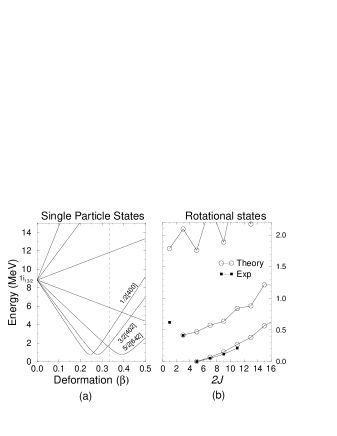
Figure 2: Energy levels for the positive parity states of ¹⁵⁷Gd. Only single-particle states from $N=6$ major shell are included. The $5/2[642]$ is below the $3/2[402]$ and $1/2[400]$ at deformations larger than 0.33. The quadrupole-quadrupole strength is set at $\kappa=0.311~{}{\rm MeV/fm}^{2}$. The black squares represent the experimental values.

For better results we include more single particle and single hole states ; two more major shells were included, the $N=5$ and $N=7$ (see Fig. 1). For $\kappa=0.23~{}{\rm MeV/fm}^{2}$ the band-head energies are in good agreement with experimental values. This change in the value of $\kappa$ was to be expected, since we are using an effective interaction. It is therefore natural to need different strengths for the interaction at different dimensions of the included single-particle space. The zig-zag shape of the $3/2^{+}[402]$ and $1/2^{+}[400]$ rotational bands reveals that the Coriolis interaction is strong compared to single particle excitations (quadrupole-quadrupole interaction) such that it creates the staggering effect. Since there are no experimental data for those bands, we cannot draw any firm conclusions concerning this behavior. The fact that the $1/2^{+}[400]$ band-head is still off by 0.3 MeV may imply that a more sophisticated interaction is needed to fully describe the structure of this band.

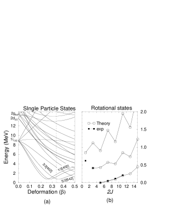
Figure 3: The positive parity energy levels of ¹⁵⁷Gd. The circles correspond to the theoretical predictions and the squares to the experimental values. The strength of quadrupole-quadrupole interaction is $\kappa=0.23~{}{\rm MeV/fm}^{2}$. Here we include states from 3 major shells.

The next step is the application of the method to the negative parity states where more data is available. The experimental situation can be summarized as follows: The ${3/2^{-}\left[521\right]}$ is the ground state band. Then follows the ${11/2^{-}\left[505\right]}$ hole band and the ${5/2^{-}\left[523\right]}$ particle band. The ${3/2^{-}\left[532\right]}$ band and the ${1/2^{-}\left[530\right]}$ band, which are not certain, are higher in energy and almost degenerate. If we only include the $N=6$ major shell, the strength $\kappa$ should be set at a value of about $0.2~{}{\rm MeV/fm}^{2}$ for the $3/2^{-}[521]$ band-head to be the ground state, which agrees with all previous calculations [31, 32]. Figure 4a shows our “Nilsson” diagram. Again particle states with lowest $K$ have lowest energy. The states deriving from the hole states obey the opposite rule; the lowest state has the highest $K$ value. In addition to this, we note that quasi-particle and quasi-hole states originating from different single particle orbitals interact weakly with each other. This leads to narrow avoided crossing between states with the same $K$ value. States with different principle quantum number $N$ also interact weakly. This is because the matrix elements $\left<r^{2}\right>$ for states having $\Delta N$ not equal to zero is smaller by a factor of the order of 10 as compared to states having the same $N$. Quasi-particle (or quasi-hole) states having angular momentum differing by four units and having the same $K$ couple strongly. For $\Delta j$ equal to 2 or 0 their interaction is weak. This is a consequence of the relevant geometric factors (three and six-j symbols). For example, the quasi-particle states of $f_{5/2}$ repel the $h_{9/2}$ states with the same $K$; as a result the band-head energies are quite sensitive to the position of the single-particle energy of the $f_{5/2}$ orbital. Because of the approximate nature of the Woods-Saxon potential, some adjustments to the single particle energy levels will be necessary for better results. The $11/2^{-}[505]$ single hole state deriving from $1h_{11/2}$ does not interact with any other state. We can easily force the $11/2^{-}[505]$ band-head to be 0.4 MeV above the ground state by lowering the $1h_{11/2}$ single-hole energy level by 1.5 MeV. Figure 4b shows the calculated band structure compared to the experimental values. The ground state band $3/2^{-}[521]$ and $11/2^{-}[505]$ band-head are reproduced very accurately. The $1/2^{-}[530]$ band-head is in good agreement with the experimental value but the rotational structure is distorted. This is due to the strong Coriolis interaction. The $5/2^{-}[523]$ and $3/2^{-}[532]$ band-heads ares way off ($\sim$5 MeV and $\sim$10 MeV respectively). At this point we can no longer improve the prediction by small adjustments of the single-particle or single-hole energies.

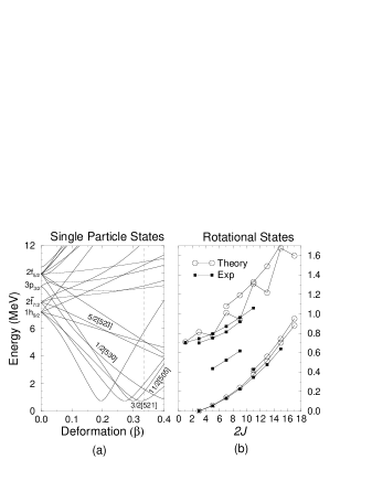
Figure 4: Negative parity states of ¹⁵⁷Gd. The squares correspond to experimental values. Only states from the $N=6$ major shell are included. The strength of the quadrupole force $\kappa$ is set to $0.201~{}{\rm MeV/fm}^{2}$.

In an attempt to improve agreement with experiment we include all single particle and hole l evels from from the $N=4$ major shell as well as intruder states from N=5 and N=7 shells. As was to be expected, the strength of the interaction must be adjusted because of the change in the size of the single particle space. For best results the quadrupole-quadrupole strength was found to be $\kappa=0.397~{}{\rm MeV/fm}^{2}$. Though it is clear why $\kappa$ is different for different dimensions, it is not clear why $\kappa$ is not the same for positive and negative parity states. For one major shell the positive parity states require $\kappa=0.31~{}{\rm MeV/fm}^{2}$ whereas for the negative parity states $\kappa=0.20~{}{\rm MeV/fm}^{2}$. For three major shells the positive parity states require $\kappa=0.2~{}{\rm MeV/fm}^{2}3$, whereas for the negative parity states $\kappa=0.39~{}{\rm MeV/fm}^{2}$. For the moment, this remains a puzzle.

The results for this more complete calculation are shown in Fig. 5 and are more satisfactory than those for one shell. The $5/2^{-}[523]$ band-head is at the right energy and the same is true for the $1/2^{-}[530]$ state. The $11/2^{-}[505]$ state is at the right position without any change to the single-particle energy spherical energy found by solving the Woods-Saxon potential. Only the $3/2^{-}[532]$ is off by $\sim 1$ MeV. The only problem is that the structure of the rotational band $1/2^{-}[530]$ is slightly distorted. This again may indicate that higher order interactions are needed to describe states of higher energy. The results are very satisfactory keeping in mind that very few free parameters were used. The most important result is that we can reproduce the rotational structure with accuracy better than any previous work, without using any attenuation or any other forms of interaction. At the same time the inclusion of the latter remains a relatively straightforward possibility

In Fig. 6 we show a similar calculation for the negative parity levels of ¹⁵⁵Gd. Single-particle states from the $N=4$, $N=6$ as well as intruder states from the $N=5$ and $N=7$ shells were included. The experimental structure of the bands is very similar to those of ¹⁵⁷Gd with the slight change in the band-head energies. The quadrupole-quadrupole strength was found to be $\kappa=0.377~{}{\rm MeV/fm}^{2}$, which is comparable to the one used for the negative parity states of ¹⁵⁷Gd. The $5/2^{-}[523]$ and the $11/2^{-}[505]$ band-heads are reproduced well. The same is true for $1/2^{-}[530]$ but the rotational structure of the band is distorted. As for ¹⁵⁷Gd, the $3/2^{-}[532]$ is off by $\sim 1.5$ MeV. The results are as good as for ¹⁵⁷Gd and the same conclusions as above apply for this nucleus.

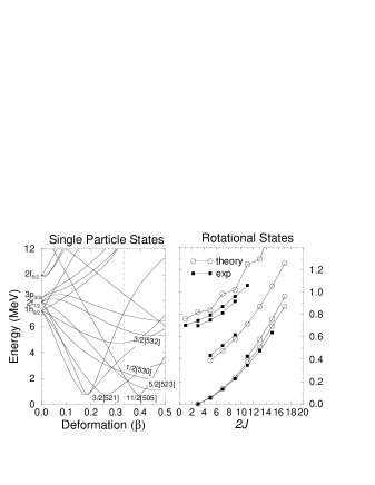
Figure 5: Negative parity energy levels ¹⁵⁷Gd. Single particle and hole states from three major shells are included. Squares correspond to the experimental values and circles to theoretical. The strength $\kappa$ of the quadrupole force is $0.397~{}{\rm MeV/fm}^{2}$.

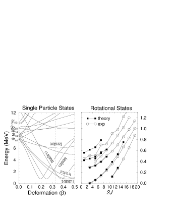
Figure 6: Negative parity energy levels for ¹⁵⁵Gd. Single particle and hole states from three major shells are included. Squares correspond to the experimental values and circles to the theoretical calculations. The strength $\kappa$ of the quadrupole force is $0.377~{}{\rm MeV/fm}^{2}$.

We have also calculated the electromagnetic transitions and compared them to experiment. In Fig. 7 we show the experimental $BE(2)$’s for ¹⁵⁶Gd and ¹⁵⁸Gd compared to the theoretical calculations using (27). The theoretical calculation represents the average of ¹⁵⁶Gd and ¹⁵⁸Gd. As can be seen from the figure the model reproduces the experiment reasonably well with some evidence of deviations at the largest angular momentum. For odd nucleus states having angular momentum $J<19/2$, the contribution of states in the even cores with angular momentum $I>12$ will be small. In the case of ¹⁵⁴Gd and ¹⁵⁶Gd we have a similar situation. Therefore, we can use either the theoretical calculations or the experimental values. Various aspects of the $BE(2)$ for transitions from $J$ to $J-2$ and from $J$ to $J-1$ are illustrated in Figs. 8-10. The experimental data are taken from [24]. The salient fact is (as was expected) that the core contribution is much larger than the single particle contribution (compare the scales in Fig. 8 with those in Fig. 9). We see that the numbers of single-particle states included only affect the single-particle contribution but not the core contribution. This shows that we are close to the extreme strong coupling limit, where the individual valence neutrons do not alter the collective behavior (core behavior). On the other hand the single particle contribution is sensitive to the number of single particle states, but if more than the major shell is included, this contribution to the $BE(2)$’s converges (Fig. 8). We have also calculated the $BE(2)$’s for different values of the effective charge. The best fit is for $e_{{\rm eff}}$ close to one. However, since the contribution of the single particle term is very small, the value of $e_{{\rm eff}}$ is of little importance. The final results of theoretical calculations for ¹⁵⁵Gd and ¹⁵⁷Gd are presented in figure 9 and 10 together with experimental data and results of other theoretical models.

Figure 7: The experimental values of $BE(2)$’s in two of the even-even Gd isotopes compared to the values calculated using Bohr-Mottelson model.

We next calculate the magnetic transitions. Here we have four parameters to fit. Because of the limitation on available experimental data for the magnetic moments of these states of ^156,158Gd, we have to use a phenomenological model for their values, [4]

$$\left<I\|M\|I\right>=g_{1}I+g_{2}I^{2},$$ (63)

where $g_{1}$ and $g_{2}$ are free parameters which we fit to the experimental points. In practice the experimental values permit a certain flexibility in the choice of these parameters. The values found by fitting the experiment in ¹⁵⁶Gd and the values used are shown in Table (1). We further adjusted $g_{1}$, $g_{2}$ and $g_{S}$ slightly in order to find the best reproduction of the experiment (see Tab. (1)). Figure 11 shows the calculations for the core contribution, the single particle contribution and the total $M1$. As can be seen from the figure, the core and single particle $M1$’s have roughly the same amplitude, and their amplitudes where chosen so as to achieve the best total $M1$.

quantity	theoretical	fit	155Gd	157Gd
$g_{1}$		$0.28\pm 0.05$	0.27	0.3
$g_{2}$		$0.018\pm 0.008$	0.019	0.02
$g_{L}$	0		0	0
$g_{S}$	-3.826		-3.586	-3.576

Table 1: The values of the parameters used for the calculations of $M(1)$’s (last two columns). The second column shows the theoretical values for $g_{L}$ and $g_{S}$, whereas the third column shows the results of a fit to ¹⁵⁶Gd for the parameters $g_{1}$ and $g_{2}$.

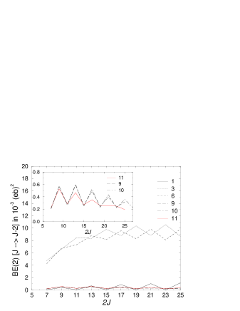
Figure 8: The single particle contribution to the $BE(2)$ ¹⁵⁷Gd for different numbers of single particle states, using $e_{{\rm eff}}=1$.

Figure 9: Comparison of our results with other models for ¹⁵⁷Gd. The formulas for the Particle-Rotor Model were taken from Ref. [4], for the Cranking model from Ref. [24]. The points with error bars are the experimental data [24], the short-dashed line is the Particle-Rotor model, the long-dashed line is the Cranking model and the solid line is the present work.

Figure 10: Comparison of our results with other models ¹⁵⁵Gd. See Fig. 9 .

Figure 11: The calculated values for the M1 for ^155,157Gd. The parameters used are are listed in Table 1. The points with error bars are the experimental data [24], the short-dashed line is the single particle contribution, the long-dashed line is the core contribution and the solid line is the total calculated $M(1)$.

4 Review of previous Work

We turn now to previous theoretical work on ^155,157Gd, in order to summarize it and compare it with our own work and with experiment. We can divide this work into three major groups according to the formulation applied.

In the papers of the first group, Refs. [6, 7, 14, 15] only band-heads are calculated, using the quasiparticle-phonon coupling scheme. In this work, the underlying physics is that of the standard core-particle coupling (CPC) model. Allowance is made for phonon excitations of the core, which can have both a quadrupole and hexadecapole deformation. The single particle states are found using a Woods-Saxon potential, and one uses a BCS approximation to include pairing correlations. In addition, interactions between states with principle quantum number differing by two are also included. Only band-heads have been calculated with this model, and the results show little improvement, as regards experiment, over calculations based on the Nilsson model, although fewer parameters are used in this approach [14]. In all these calculations the Coriolis interaction is neglected. The argument is that the Coriolis interaction has only a slight effect on the energies and structures of the lowest parts of the rotational bands [6, 7]. The results of the best two calculations of this type are compared with experiment and with our calculations in Fig.  12.

The second group, Refs.[12, 13, 8, 9] contains complete calculations of the rotational spectrum in the standard core-particle coupling model. Early works based on this model utilize a rotating deformed core which is coupled to a single odd nucleon. The mean field from the core is represented by a Nilsson potential. The coupling between the core and the odd nucleon, the Coriolis coupling, is treated as a perturbation (strong coupling limit). In Ref [12, 13] a deformed Woods-Saxon potential is considered. Again, pairing is taken into account by means of a BCS transformation. Another extension of the original model takes into account mixing between different major shells [12, 13]. In Fig. 13 we show the experimental values compared to three theoretical models. The first one (Fig. 13b) is from [12]. In this paper the model Hamiltonian includes a quadrupole and hexadecapole deformed core. The pairing is treated in BCS approximation. The deformation parameters $\beta_{20}$, $\beta_{40}$ and the moment of inertia ${\cal I}$ are taken as freely adjustable parameters. The set of results shown in Fig. 13c is from Ref. [13]. In this paper the same Woods-Saxon potential and BCS approximation are used. The model contains two additional free parameters: the moment of inertia and the Coriolis attenuation factor $\kappa$, which was found to be 0.63. The last part of Fig. 13 is based on our results, without any Coriolis attenuation.

Figure 12: Negative parity band-head energies for ¹⁵⁷Gd from: (a) experiment, (b) reference [6], (c) reference [7], (d) our work.

Figure 13: Negative parity states for ¹⁵⁷Gd from: (a) experiments, (b) reference [12], (c) reference [13], (d) our work.

The third group includes models based on dynamical symmetry arguments; the pseudo SU(3) [33] and the interacting boson-fermion approximation (IBFA) [34]. The results are reasonable for both models but they will not be reviewed because they describe only the lowest bands.

5 Conclusions

In this paper we have applied to ^155,157Gd the Core-Particle model as originally formulated by Klein and co-workers and modified for practical application by Dönau and Frauendorf. When levels from several major shells were included, the band-heads were predicted quite satisfactorily. The rotational structure is predicted with high accuracy and only the higher bands are distorted. We believe that the reason for this distortion is the Coriolis interaction which is included naturally in the core Hamiltonian ($H_{c}$). The standard approach to this difficulty is to attenuate the Coriolis interaction [12, 13]. Since there is no justification for this ad-hoc procedure, the best approach is to include other forms of interaction which will counteract this effect. The suggested candidates are the quadrupole-pairing and hexadecapole-hexadecapole interactions, which will be investigated in the further development of this work.

The electric transitions $BE(2)$ were predicted and the results are closer to the experimental values than any other theory for which comparisons have been made. For the magnetic transitions $M(1)$ we reproduce the experiment but need 4 parameters to do so. These parameters are not fully constrained by experiment.

Finally, it may be useful to summarize in general what has been accomplished and how the model may be extended. In our approach, the kinematical Coriolis coupling between the particle and the core is automatically included. There is in fact no natural way of introducing an ad-hoc attenuation, for which we have found little evidence. There is some indication in higher excited bands, but not enough data is available to substantiate this. In our calculations an excessive influence of this coupling can be dealt with only by modifying the effective interaction. In addition non-adiabatic corrections to the treatment of the core may be studied, either by use of experimental matrix elements or by calculating higher order corrections to the Bohr-Mottelson theory. Finally to study experimental results at higher angular momentum, we must include excited bands of the core. Because of the modest success of the calculations reported in this paper, we feel encouraged to continue our investigations along the lines suggested above.

6 Acknowledgement

This work was supported in part by U.S. Department of Energy under grant number 40264-5-25351

References

- [1] A. Klein and A. Kerman, Phys. Rev. 132, 1326 (1963).
- [2] A. Klein, Phys. Rev. C 30, 1960 (1984).
- [3] A. Klein and N. R. Walet, in International Workshop Nuclear Structure Models, edited by R. Bengtsson, J. Draayer, and W. Nazarewicz (World Scientific, New York, 1992), p. 229.
- [4] A. Bohr and B. R. Mottelson, Nuclear Structure, Vol. 2 (Benjamin, New York, 1975).
- [5] F. Dönau and S. Frauendorf, Phys. Lett. B 71, 263 (1977).
- [6] F. A. Gareev, V. G. Solov’ev, and S. I. Fedotov, Sov. J. Nucl. Phys 14, 646 (1972).
- [7] F. A. Gareev, S. P. Ivanova, V. G. Solov’ev, and S. I. Fedotov, Sov. J. Part. and Nucl. 4, 148 (1973).
- [8] K. Jain and K. A. Jain, Phys. Rev. C 30, 6 (1984).
- [9] P. C. Josh and P. C. Sood, Phys. Rev. C 9, 5 (1974).
- [10] V. G. Solov’ev and P. Vogel, Nucl. Phys. A 192, 446 (1967).
- [11] M. K. Kolpazhiu and P. Vogel’, Izv. A. SSSR, Ser. Fiz 30, 2025 (1966).
- [12] B. Hird and K. H. Huang, Can. J. Phys. 53, 6 (1975).
- [13] R. Katajanheimo and E. Hammaren, Physica Scripta 19, 497 (1979).
- [14] L. A. Malov, V. G. Solov’ev, and S. I. Fedotov, Bull. Acad. Sci. USSR, Phys. Ser. 35, 686 (1972).
- [15] B. A. Alikov, K. Zuber, V. V. Rashkevich, and E. A. Tsoi, Bull. Acad. Sci. USSR, Phys. Ser. 48, 5 (1984).
- [16] J. Almenger and et al, Physica Scripta 22, 331 (1980).
- [17] G. A. Leander and Y. S. Chen, Phys. Rev C 37, 2744 (1988).
- [18] R. Bengtsson and et al., Annual report 1987-1988, Department of Mathematical Physics, Lund Institude of Technology.
- [19] P. B. Semmes, in International Workshop Nuclear Structure Models, edited by R. Bengtsson, J. Draayer, and W. Nazarewicz (World Scientific, New York, 1992), p. 287.
- [20] F. Dönau, in Mikolajki Summer School of Nuclear Physics, edited by Z. Wilhelmi and M. Kicinska-Habior (Harwood Academic, New York, 1986).
- [21] F. Dönau, in Nordic Winter School on Nuclear Physics, edited by T. Engeland, J. Rekstad, and J. S. Vaagen (World Scientific, Singapore, 1984).
- [22] F. Dönau and S. Frauendorf, Phys. Lett. 71B, 263 (1977).
- [23] F. Dönau and S. Frauendorf, J. Phys. Soc. Japan (Suppl) 44, 526 (1977).
- [24] H. Kusakari et al., Phys. Rev C 42, 1257 (1992).
- [25] A. Klein, Adv. in Part. and Nucl. Phys 10, 39 (1983).
- [26] G. D. Dang et al., Nuc. Phys. A 114, 39 (1968).
- [27] D. Cebula, A. Klein, and N. R. Walet, J. Phys. G 18, 499 (1992).
- [28] D. Cebula, A. Klein, and N. R. Walet, Phys. Rev. D. 47, 2113 (1993).
- [29] P. Ring and P. Shuck, The Nuclear Many Body Problem (Springer, Berlin, 1980).
- [30] S. Raman, C. W. Nestor, and K. H. Bhatt, Phys Rev C 37, 2 (1988).
- [31] D. R. Bes and R. A. Sorensen, in Advances in Nuclear Physics 2, edited by M. Baranger and E. Voght (Plenum Press, New York, 1969), p. 129.
- [32] P. J. Brussaard and P. W. M. Glaudemans, Shell-model applications in nuclear spectroscopy (North-Holland, Amsterdam, 1977).
- [33] S. Thalluri and R. D. R. Raju, J. Phys. G: Nucl. Phys. 6, 803 (1980).
- [34] R. D. R. Raju, J. P. Draayer, and K. T. Hecht, Nucl. Phys. A 202, 433 (1973).