UNIVERSITY of PENNSYLVANIA
Department of Physics David Rittenhouse Laboratory Philadelphia PA 19104–6396

PREPRINT UPR–0408T-R

Extracting Nuclear Transparency from p-A Cross sections

Sherman Frankel, William Frati, and Niels R. Walet

Submitted to Nuclear Physics A

Abstract

We study nuclear structure effects on the transparency in high transverse momentum $(p,2p)$ and $(e,e^{\prime}p)$ reactions. We show that in the DWIA-eikonal approximation, even when correlations are included, one can get a factorized expression for the transparency. This depends only on the average nucleon density $\rho(r)$ and a correlation function. We develop a technique to include correlations in a Monte-Carlo Glauber type calculation. We compare calculations of $T$ using the eikonal formalism and a continuous density, with a Monte Carlo method based on discrete nucleons.

1 Introduction

High $p_{t}$ $(p,2p)$ interactions in nuclei have gained renewed interest following the suggestion [1] that fluctuations in nucleon size may show observable effects due to color screening. Of particular interest is the nuclear transparency, $T$, which is defined as the probability that a proton traversing a nucleus makes one and only one collision with a nucleon and that the emerging nucleons make no further interactions. It can apply to any interaction, but in this paper we consider the case where the basic interaction is either a proton-proton or an electron-proton interaction. The transparency is extracted from the experimentally obtained quasielastic $(p,2p)$ events using the factorization assumption [2, 3]:

$$\frac{d}{dt}\sigma_{p-A}/Z=T\int S(\vec{k},\epsilon,\sigma_{tot})\frac{d}{dt}\sigma_{\rm p-p}(s,t)d^{3}kd\epsilon$$ (1)

This is the expression found in Eq. (2) of Ref. [3]. In this factorized form $\sigma_{\rm p-p}$ is the $(p,2p)$ cross section evaluated at the appropriate Mandelstam variables, $s$ and $t$. The variable $s(k,\epsilon)$ is the on-shell center-off-mass energy which is a function of the missing energy, $\epsilon$, and missing momentum, -$\vec{k}$, measured from the kinematic reconstruction of the $(p,2p)$ events, and $t$ is the measured 4-momentum transfer. Finally $S(\vec{k},\epsilon,\sigma_{tot})$ is a spectral function, which depends on the proton-nucleon interaction cross section, $\sigma_{tot}$, and on the spatial distribution of nucleons in the nucleus. It is normalized to unity.

Using Eq. (1) $T$ can be extracted from the experimental data by weighting each observed event with the reciprocal of $\frac{d}{dt}\sigma_{\rm p-p}(s,t)$, to remove the dependence of $T$ on $\vec{k}$ and $\epsilon$. For an experiment designed to accept events of any momentum $\vec{k}$ and missing energy $\epsilon$ there is no need to know $S(\vec{k},\epsilon,\sigma_{tot})$, since $\int S(\vec{k},\epsilon,\sigma_{tot})d^{3}k\,d\epsilon=1$. In practice, at incident momenta of 6-10 GeV which are much larger than the average $k$, corrections for apparatus acceptance as a function of $\vec{k}$ are not difficult to obtain, especially since $S$ falls rapidly with $k$.

If there were no initial state or final state interactions of the protons traversing the nucleus, $T$ would be unity. Thus $T$ measures these initial and final state interactions which are sensitive to the total proton-nucleon cross section, $\sigma_{tot}$, which in turn will depend on the magnitude of the color screening. One of the important ideas in color transparency is that $T$ will increase with the momentum transfer, $t$, observed in the $(p,2p)$ reaction. Thus we examine how to determine $T(t)$ in a way that will depend least on theoretical calculations of its magnitude. This is also of value since it bypasses the strong sensitivity of $T$ to the nucleon density near the nuclear edge. (In general only a peripheral reaction will have a single scattering, so that edge effects are enhanced.) We examine the special case of the $t$ dependence of the nuclear cross section as measured in a $(p,2p)$ reaction where the exiting protons are observed at the angles $\theta_{1}$ and $\theta_{2}$.

In this paper we show that a factorized expression for $T$, Eq. (1), can be derived from the Distorted Wave Impulse Approximation. By using the closure approximation, as employed by Lee and Miller [4], the spectral function $S$ becomes independent of $\epsilon$ (we denote this simplified function by $J$ in this work). Even with this additional approximation, the expression for the cross section is rather complicated, see Ref. [4]. However, we show that the transparency depends only the nuclear proton radial distribution $\rho(r)$. The density $\rho$ can be obtained from elastic $e-A$ scattering without recourse to knowledge of the individual single particle wave functions. After using closure the transparency $T$ turns out to be related to the classical probability that there are no initial or final state scatters accompanying the $(p,2p)$ high $p_{t}$ interaction on a single nucleon. We shall see later how to take into account both the momentum and missing energy taken off by the undetected nucleons measured in a fully reconstructed $(p,2p)$ experiment.

We also show how the effect of nucleon correlations, which affect the calculation of $T$, can be included in a previously developed Monte-Carlo formalism for Glauber scattering, and compare various model assumptions with the data.

We also discuss the transparency in the $(e,e^{\prime}p)$ reaction, for which both theoretical [5] and experimental studies [6] have been performed. The formalism developed by Benhar et al. closely parallels the DWIA eikonal formalism used by Lee and Miller.

2 Transparency and the Distorted Wave Impulse Approximation

Let us first review the expected cross section on the basis of the plane wave impulse approximation (PWIA). This cross section can be obtained by using the closure approximation to sum over final states and using on-shell values of the Mandelstam variables, $s$ and $t$, for the quasi-free interaction [4]. The result of this quantum-mechanical approximation is to obtain a simple limit: The cross section, for an incident proton of energy, $E_{0}$, on a nucleon with wave function $\psi$ becomes the probability, $P(k)$, of finding that nucleon in the nucleus with momentum $k$, times the $(p,2p)$ cross section at the on-shell values of $s(E_{0},\vec{k},\epsilon)$ and the momentum transfer, $t$. While $t$ is directly obtainable from the measured momenta, $\vec{k}$ and $\epsilon$ refer to the momentum and binding energies in the initial state which are not directly measurable.

For interaction with a single nucleon of independent particle wave function $\psi$, the result is well known [4]:

$$\frac{d\sigma_{p-A}}{dt}/Z=\int P(k)\frac{d\sigma_{\rm p-p}[s(k,\epsilon,t)]}{dt}d^{3}k.$$ (2)

In particular $P(k)=|F(k)|^{2}$ where $F(k)$ is the Fourier transform of the nucleon wave function, $\psi(r)$,

$$F(k)=\int e^{i\vec{k}\cdot\vec{r}}\psi(\vec{r})d^{3}r.$$ (3)

It is useful to recall that, in Eq. (3), the wave function, $\psi(\vec{r})$, must be normalized to unity in order that $\int P(k)d^{3}k$ give the proper total probability, i.e., $\int P(k)d^{3}k=1$.

We next examine the cross section in the distorted wave impulse approximation (DWIA). In this approximation the plane waves for the incoming $(i=0)$ and outgoing $(i=1,2)$ particles are replaced by distorted waves of the form $e^{i(\vec{p}_{i}\cdot\vec{r})}D_{i}(\vec{r},\rho(r),\sigma_{tot},\vec{p}_{i})$, where $D_{i}$ is a factor describing the distortion of the plane wave. It depends on the total p-nucleon cross section $\sigma_{tot}$, the nuclear density $\rho$ and the momentum of the $i$th proton $\vec{p}_{i}$.

For the case of a single filled orbital we find that $F(k)$ in Eq. (3) is replaced by $F^{\prime}(\vec{k})$,

$$F^{\prime}(\vec{k})=\int e^{i\vec{k}\cdot\vec{r}}D_{0}D_{1}D_{2}\psi(\vec{r})d^{3}r.$$ (4)

Note that since in general the $D$’s are not rotationally invariant the momentum distribution no longer depends only on the magnitude of $k$ but depends on both the transverse momentum, $k_{t}$, and longitudinal momentum, $k_{z}$.

In order for $P^{\prime}(k)=|F^{\prime}(\vec{k})|^{2}$ to be a proper effective momentum distribution which includes the initial and final state interactions, $F^{\prime}(k)$ must be normalized so that $\int P^{\prime}(k)d^{3}k$ is unity. The normalization factor needed in Eq. (4) is defined as $\sqrt{T}$, anticipating the result displayed in Eq. (7), and is given by:

$$T=\int\ D_{0}D_{1}D_{2}\psi(\vec{r})^{*}D_{0}D_{1}D_{2}\psi(\vec{r})d^{3}r,$$ (5)

so that

$$P^{\prime}(k,\sigma)=\left|\frac{\int e^{i\vec{k}\cdot\vec{r}}D_{0}D_{1}D_{2}\psi(\vec{r})d^{3}r}{\sqrt{T}}\right|^{2}.$$ (6)

We then find, in analogy with (2),

$$\frac{d\sigma_{p-A}}{dt}/Z=T\int P^{\prime}(k)\frac{d\sigma_{\rm p-p}[s(k,\epsilon,t)]}{dt}d^{3}k.$$ (7)

The p-p cross section can be obtained from p-p data where $s$ is determined from $k$ and $\epsilon$, which in their turn are obtained by kinematically reconstructing each event under the assumption that all the accepted events are pure $(p,2p)$ events with no initial and final state rescatterings.

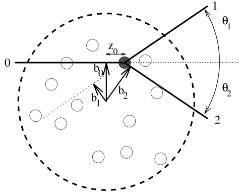
Figure 1: Geometry of the scattering process. The vectors $\vec{b}_{i}$ are the impact parameters for each of the three paths (0 labels the incoming path, 1 and 2 label the two outgoing paths) for a collision taking place at a nucleon at $\vec{r}$. $z_{0}$, and equivalently $z_{1}$ and $z_{2}$, are the $z$ coordinates of $\vec{r}$ in the $\vec{b},z$ coordinate systems. $\theta_{1}$ and $\theta_{2}$ are the angles of the outgoing protons relative to the incoming proton direction.

In order to obtain the DWIA expression for $T$ we follow Lee and Miller and use the eikonal form of $D$ to evaluate $T$. With the path lengths, $z$, defined in Fig. 1 ($z_{0}$ along the direction of the incoming particle, $z_{1}$ and $z_{2}$ along the trajectories of the outgoing particle) we have:

$$D_{0} = \exp\left[{-\int_{-\infty}^{z_{0}}\frac{\sigma_{tot}}{2}\rho(z,\vec{b}_{0})dz}\right],$$

$$D_{1} = \exp\left[{-\int_{z_{1}}^{\infty}\frac{\sigma_{tot}}{2}\rho(z^{\prime},\vec{b}_{1})dz^{\prime}}\right],$$

$$D_{2} = \exp\left[{-\int_{z_{2}}^{\infty}\frac{\sigma_{tot}}{2}\rho(z^{\prime\prime},\vec{b}_{2})dz^{\prime\prime}}\right].$$ (8)

Inserting these expressions in Eq. (5) we obtain:

$$T=\int e^{-\int_{-\infty}^{z}\sigma_{tot}\rho(\vec{r})dz_{0}}e^{-\int_{z}^{\infty}\sigma_{tot}\rho(\vec{r})dz_{1}}e^{-\int_{z}^{\infty}\sigma_{tot}\rho(\vec{r})dz_{2}}\rho(\vec{r})d^{3}r=\int P_{0}P_{1}P_{2}\rho(r)d^{3}r.$$ (9)

The functions $P_{i}$, that are the squares of the functions $D_{i}$ in (8), can be interpreted as the probability that there are no interactions in the leg $i$ of the reaction.

In general we have several (partially occupied) orbits in a shell-model nucleus. The result found here remains true, however. Let us consider the example of two completely filled levels, $s$ and $p$, with equal occupation numbers. We define the “normalized to unity” effective momentum distribution for state $i$ ($i=s,p$) by

$$f_{i}(k)=\left|\int e^{i\vec{k}\cdot\vec{r}}D_{0}D_{1}D_{2}\psi_{i}(\vec{r})d^{3}r\right|^{2}/~{}T_{i},$$ (10)

with the normalization factor determined from:

$$T_{i}=\int[(D_{0}D_{1}D_{2}\psi_{i}(\vec{r})]^{*}[D_{0}D_{1}D_{2}\psi_{i}(\vec{r})]d^{3}r.$$ (11)

We then have the useful form:

$$\sigma_{p-A}/Z=(T_{s}+T_{p})\int\left[\frac{f_{s}T_{s}+f_{p}T_{p}}{T_{s}+T_{p}}\right]\times\sigma_{\rm p-p}(s,t)d^{3}k.$$ (12)

Note that $T_{s}+T_{p}$ is identical with $T$ since

$$T_{s}+T_{p}=\int(D_{0}D_{1}D_{2})^{2}[\psi_{s}(r)^{*}\psi_{s}(r)+\psi_{p}(r)^{*}\psi_{p}(r)]d^{3}r=\int(D_{0}D_{1}D_{2})^{2}\rho(r)d^{3}r.$$ (13)

This result can easily be extended to more independent particle states and is the basis for our result that only $\rho(r)$ is needed to calculate $T$. Thus Eq. (13) is identical with Eq. (9).

Note also the useful relation for the momentum distribution, resulting from our normalization of $f$:

$$\int J(\vec{k},\sigma)d^{3}k\equiv\int\left[\frac{f_{s}T_{s}+f_{p}T_{p}}{T_{s}+T_{p}}\right]d^{3}k=1.$$ (14)

The final form can thus be written:

$$\frac{d}{dt}\sigma_{p-A}/Z=T\int J(\vec{k},\sigma)\frac{d}{dt}\sigma_{\rm p-p}(s,t)d^{3}k.$$ (15)

Thus, as in the PWIA, the DWIA also leads to a cross section that can be factored into an effective normalized momentum distribution, $J(\vec{k})$, and a $k$ independent quantity, $T$, called the transparency. This result relies on the use of a closure approximation, so that there are no interference terms in Eq. (12). Let us repeat this equation (9) once more, since it is one of the important results of this paper: $T=\int P_{0}P_{1}P_{2}\rho(r)d^{3}r$. Thus we recognize that the normalization factor in Eq. (5) is in fact just the transparency in Eq. (9)! This equation is exactly the expression for $T$ used by Farrar et al. [7] in their calculations.

Eq. (9) can be understood as the probability that there is no nuclear interaction of the incoming or outgoing protons along the paths $z_{0},z_{1}$ and $z_{2}$ determined by $\vec{r}$, $\theta_{1}$, and $\theta_{2}$. However it does not include “nuclear correlation” effects that modify $\rho(r)$ in Eq. (9) in the neighborhood of the struck nucleon. These corrections were calculated in Ref. [8] and are discussed and included by Lee and Miller [4]. We have also calculated this probability using a Monte Carlo method which automatically [8] excludes the nucleon participating in the high $p_{t}$ $(p,2p)$ interaction from the absorptive path.

Equations (9) and (15) allow $T$ to be determined directly from the proton charge density, $\rho(r)$, which can be obtained from elastic e-nucleus scattering rather than requiring a detailed knowledge of the ground-state wave functions for all the nucleons of a complicated nucleus, which is the procedure followed in Ref. [4].

The correlations of the struck nucleon with its surroundings make it less plausible to find another particle very close to this nucleon. This can be most simply be taken into account by replacing the one-body density $\rho$ in all three equations (8) by the probability to find a particle at position $\vec{r}_{zb}$ along one of the three legs, if there is one at the beginning (at position $r$),

$$\rho_{2}(\vec{r},\vec{r}_{zb})/\rho(r)\equiv\rho(r_{zb})C(\vec{r},\vec{r}_{zb}).$$ (16)

Here we have defined a correlation function $C$. This entity is usually approximated by the result of a nuclear matter calculation. As is argued in the appendix, however, this correlation function should also take into account the $(A-1)/A$ corrections arising from the fact that one should not include the struck nucleon among the absorbing material. Thus, for no correlations, we find $C=(A-1)/A$, which for light nuclei gives a considerable correction to the transparency.

3 The “Glauber” Calculation of $T$

The Glauber model has proved to be quite successful in understanding p-A and heavy ion interactions at high energies ($>$ 5 GeV). The basic quantities such a calculation are the so-called Glauber coefficients, $a_{n}$. The coefficient $a_{n}$ gives the probability that a proton makes $n$ collisions in traversing a nucleus, while remaining on a straight path (this assumption is similar to the eikonal approximation). One approximate way for obtaining the Glauber coefficients is based on a Monte-Carlo generations of particles in a nucleus. One first generates the positions of nucleons in a nucleus randomly, according to the nuclear density $\rho(r)$. One then follows the path of the incoming proton through the nucleus, and counts the number of collisions. The collisions are treated geometrically, and are assumed to take place whenever the impact parameter for the incoming proton and any target nucleon is less than $b_{\sigma}$ obtained from the proton-nucleon cross section, with $\sigma_{tot}=\pi b_{\sigma}^{2}$. The number of collisions is thus equal to the number of centers of particles in a cylinder of radius $b_{\sigma}$ around the path of the projectile, see Fig. 2.

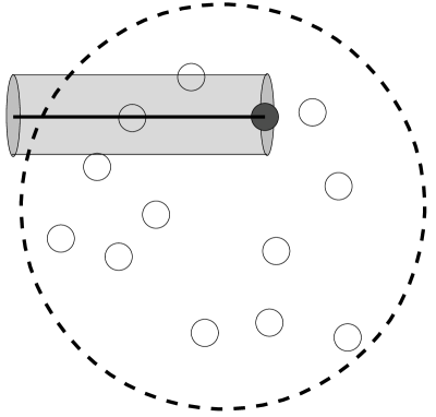
Figure 2: The geometrical cylinder where no particles are allowed for a transparent reaction. For the calculation of $a_{n}$ we draw a cylinder through the whole nucleus and count the number of particles inside. Here we have illustrated one of the legs in the $(p,2p)$ scattering, centered on the particle where the hard collision is made. We construct a similar cylinder for each of the three legs.

Here we have taken into account the fact that at very high energies the path of the incoming particle through the nucleus can be approximated by a straight line. Such a probabilistic calculation of the $a_{n}$ is known to be equivalent to the quantum mechanical Glauber model in the case of factorized ground state densities [9] and has been used over the last decade to determine the $a_{n}$ which are used in models that study multiplicities [10, 11], $E_{t}$ distributions [12, 13], leading hadron distributions [14] and many other measured quantities in p-A and heavy ion collisions at high energies.

For our transparency calculations we need determine the probability that if the projectile nucleon makes a large-angle $(p,2p)$ scatter, no other soft collisions take place. We sum over all particles in the nucleus, and assume that the hard-collision takes place at one particle at a time. We then look at the incoming path, and also follow the paths of the two final state protons, and look whether a geometric scattering takes place along each path. We allow the nucleons to scatter into non-zero angles as determined by the $(p,2p)$ kinematics. The calculation is similar but not identical with the eikonal-DWIA calculation discussed in the previous section. The expression for $T$ resembles Eq. (9) with the exponential factor $P_{i}$ replaced by the probability that there are no other interactions except the hard $pp$ interaction along the appropriate path.

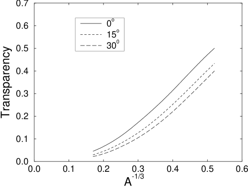
Figure 3: The transparency calculated as a function of $A$ for the Glauber Monte Carlo model. The three curves represent three different laboratory angles for the $pp$ scatter.

In figure 3 we show the dependence of the transparency on the laboratory angle of the $pp$ scatter. The kinematics are usually chosen so that the cm scattering angle is $90^{\circ}$, we see that the transparency increases trivially as the energy increases. We have used $\sigma_{\rm tot}=37~{}{\rm mb}$, which we consider to be a reasonable value for the high-energy $pp$ cross-section in nuclei. This value will be used in all calculations in this paper.

One basic difference between this Glauber calculation and the DWIA calculation is that the Monte Carlo treats the nucleus as composed of confined nucleons of finite volume while the DWIA treats a continuous matter distribution. We believe that at 10 GeV, where the wavelength of the projectile is smaller than the nucleon diameter, one cannot neglect the “lumpiness” of the nuclear medium. In contrast to the eikonal calculation discussed in the previous section, in the Glauber calculation the target nucleon participating in the hard $(p,2p)$ scatter is by definition not counted in the absorptive path. This does not mean that nuclear correlations do not have an effect on the result of the Glauber calculation, but the effect can be different. Let us investigate the generation of correlated nuclei using our Glauber-Monte Carlo algorithm.

3.1 Monte Carlo generation of particles

As in the Eikonal-DWIA calculations we wish to use a nuclear matter calculation as a guide to construct a correlated sampling of a finite nucleus. There are several reasons why we cannot use a correlation function directly as input to the calculation. The most important reason is the fluid nature of the nuclear many-body system, which induces many-particle correlations.

3.1.1 Nuclear matter

Let us first look at the case of nuclear matter. If we consider particles with only two-body interaction, one expects that the probability of finding the particles can be written as a product of two-body correlation factors,

$$\rho(\vec{r}_{1},\ldots)=\prod_{i}\rho\prod_{i<j}g(|\vec{r}_{i}-\vec{r}_{j}|)$$ (17)

where $g$ is a two-body correlation factor. This function should approach one for large separations. The point is that, for nuclear matter, the correlation length – the distance in which $g(r)$ approaches one – is comparable to the internucleon spacing. This means that in general we will be able to find triples of particles ($\vec{r}_{i}$, $\vec{r}_{j}$, $\vec{r}_{k}$) in the Monte-Carlo sample such that at least two of the three $g$’s ($g(\vec{r}_{i}-\vec{r_{j}})$, $g(\vec{r}_{i}-\vec{r_{k}})$ and $g(\vec{r}_{j}-\vec{r_{k}})$) differ significantly from one. This leads to effective (induced) three-body correlations. If we now calculate the two-particle distribution, the probability to find one particle at $\vec{r}_{1}$ and another at $\vec{r}_{2}$,

$$\rho_{2}(\vec{r}_{1},\vec{r}_{2})=\rho^{2}C(|\vec{r}_{1}-\vec{r}_{2}|),$$ (18)

we find that the function correlation function $C$ is in general different from $g$. (Note that in the low-density (gas) approximation $C=g$.) This can be seen in Figs. 4 and 5 for two choices of the function $g$. We have used a Monte-Carlo algorithm where we generate N particles in a square box with periodic boundary conditions.

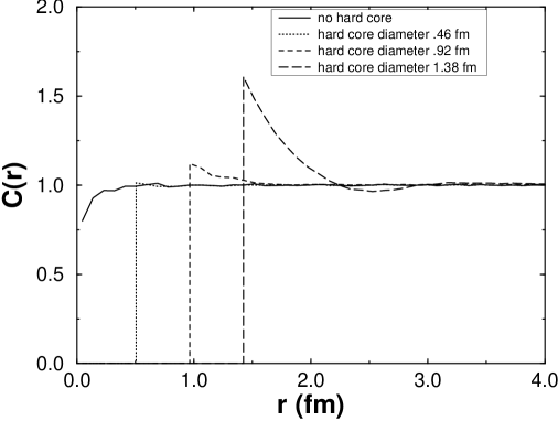
Figure 4: The effect of hard-core correlations in “nuclear matter”, on the correlation function $C$, for various hard-core radii. The solid line is 0 hard core radius. In sequence the other three lines have a hard-core diameter of .46, .92 and 1.38 fm.

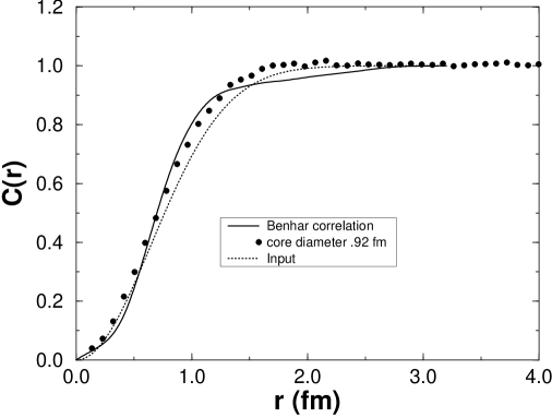
Figure 5: The effect of a Gaussian correlation in “nuclear matter”, on the correlation function $C$. The dashed line is the input Gaussian, the solid line the correlation function used by Benhar et al. The black circles represent the outcome of a Monte-Carlo calculation.

In Fig. 4 we show the effect of a hard-core interaction,

$$g(r)=\left\{\begin{array}[]{lr}0&r<R\\ 1&r>R\end{array}\right..$$ (19)

As one can see the resulting curves do not have very much in common with the results of more standard nuclear matter calculations (see Fig. 5). The hard core reduces the available positions in configuration space so that for the large core radii each particle is surrounded by a number of particles that almost touch. This leads to the strong peak in the correlation function for $r=R$. In Fig. 5 we use a Gaussian $g$,

$$g(r)=1-\exp(-(r/R)^{2}).$$ (20)

This function results in a $C$ that – for $R=.92~{}{\rm fm}$ – is very similar to the realistic correlation function used by Benhar et al. [5] in their calculation for the $(e,e^{\prime}p)$ transparency. This is what we use in our further calculations.

3.1.2 Finite nuclei

Whereas for infinite nuclear matter we can have an arbitrary, but translationally invariant, correlation function, the correlation function for finite nuclei must satisfy a normalization condition. This follows from the equation

$$\int d^{3}r_{2}\rho^{2}(\vec{r}_{1},\vec{r}_{2})=(A-1)\rho(\vec{r}_{2}),$$ (21)

which after the substitution

$$\rho^{2}(\vec{r}_{1},\vec{r}_{2})=\rho(\vec{r}_{1})C(\vec{r}_{1},\vec{r}_{2}\rho(\vec{r}_{2})$$ (22)

becomes

$$\int d^{3}r_{2}C(\vec{r}_{1},\vec{r}_{2})\rho(\vec{r}_{2})/(A-1)=1.$$ (23)

We obviously also require that the one-body distribution coming from the Monte-Carlo generation takes on the form $\rho(\vec{r})$.

We wish to develop an approach to finite nuclei that is close in spirit to the nuclear matter calculation discussed in the previous subsection. Therefor we use an approach based on two-body correlation factors. We use a $N$-particle distribution $\rho$ of the form

$$\rho_{N}(\vec{r}_{1},\ldots,\vec{r}_{N})={\cal N}\prod_{i=1}^{N}\zeta(r_{i})\prod_{i<j}^{N}g(|\vec{r}_{i}-\vec{r}_{j}|).$$ (24)

${\cal N}$ is a normalization factor, that could be absorbed in the effective single particle densities $\zeta$. The function $\zeta$ is chosen such that $\rho(\vec{r})$ takes a given form (usually Wood-Saxon), whereas $g$ is taken to be identical to the nuclear matter result. For a dilute gas one find that $\zeta=\rho$ and $g=C$. Unfortunately a nucleus is more like a fluid than a gas, so that we have to solve for $\zeta$.

In this work we require that for $g$ given by Eq. (20) we obtain a Wood-Saxon density,

$$\rho(r)\propto\frac{1}{1+\exp([r-R_{0}]/\sigma)},$$ (25)

with $\sigma=.545~{}\rm fm$ and $R_{0}=1.14A^{1/3}~{}\rm fm$. It is rather complicated to solve the many-body problem for $\zeta$. We found it convenient to use a parametrized form and look for a set of parameters that yields a result that closely resembles a Wood-Saxon. A form that seems to be sufficient for this goal is

$$\zeta(r)\propto\frac{1}{\left(1+\exp([r-R^{\prime}_{0}]/\sigma^{\prime})\right)\left(1+\alpha r\right)}.$$ (26)

The function $\zeta(r)$ is a parent distribution, from which we chose particles in the Monte-Carlo calculation. If we include the correlation factors $g$ (by a rejection technique) this leads to a single particle distribution of the desired form $\rho(r)$.

To illustrate the accuracy obtained by using (26) to arrive at the Wood-Saxon distribution (25), we show a few of the results of our calculations in Fig. 6. The relevant parameters for a few nuclei are given in Table 1.

Table 1: The parameters of $\zeta$, Eq. 26 for a few nuclei, as determined from a Monte-Carlo calculation.

$A$	$R_{0}$ (fm)	$R_{0}^{\prime}$ (fm)	$\sigma^{\prime}$ (fm)	$\alpha$ (1/fm)
7	2.18	2.18	.545	0.10
12	2.61	2.55	.545	0.13
16	2.87	2.75	.545	0.16
40	3.90	3.70	.545	0.19
100	5.29	4.90	.540	0.19
208	6.75	6.17	.530	0.19

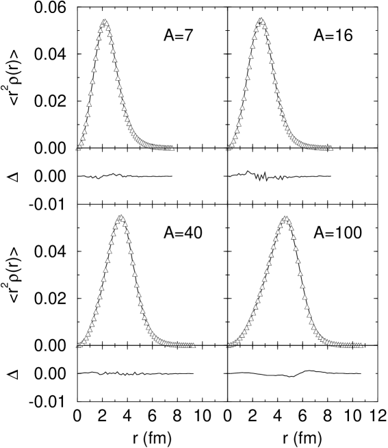
Figure 6: A comparison of the result of the density for the correlated Monte-Carlo result to a Wood-Saxon, for four different nuclei. For each pair of graphs the upper one shows the value of the single-particle distribution in a set of bins. The triangles are the Monte-Carlo results, and the drawn line is the exact result for a Wood-Saxon distribution. The lower graph shows the difference, $\Delta$, between the two sets of results. For parameters see Table 1.

4 Model Dependence of $T$

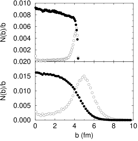
Figure 7: Impact parameter dependence of collisions in ⁶⁴Cu. Filled circles denote the number of all scatters vs. the impact parameter, $b$. Open circles give the number of transparent collisions multiplied by ten. Both figures use a Woods-Saxon density. The upper figure has very small diffuseness, $\sigma=.005~{}{\rm fm}$, the lower has a realistic diffuseness, $\sigma=.545~{}{\rm fm}$.

To elucidate the sensitivity of $T$ to the shape of the nuclear surface we show in Fig. 7 the dependence of $N(b)/b$, the number of collisions at impact parameter, $b$, versus $b$. Superimposed on the same figure is the plot for the number of pure $(p,2p)$ events, i.e., those without initial or final state scattering, $T(b)$ (multiplied by 10). These curves illustrate how the tail of the $N(b)$ distribution determines both the shape and position of $T(b)$. Nost of the transparent events take place where the nuclear density is about $1/4$ of the maximum density.

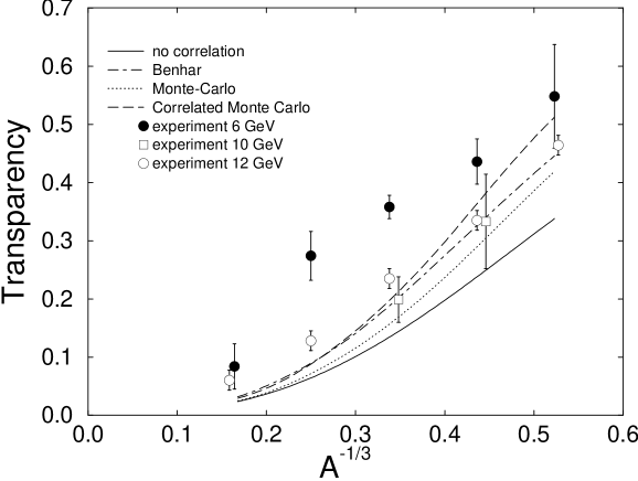
Figure 8: The transparency for the $(p,2p)$ reaction calculated using various methods. The angles $\theta$ have been chosen appropriate to a geometry corresponding to $90^{\circ}$ scattering in the cm frame for $E_{lab}=10~{}{\rm GeV}$. The 6, 10, and 12 Gev data are from Ref. [2].

In Fig. 8 we compare the results of various calculational schemes discussed in this paper. We have calculated the transparency in $(p,2p)$ reactions for the methods discussed in the previous sections, all using a Wood-Saxon density of the form

$$\rho(r)\propto\frac{1}{1+\exp[(r-R_{0})/\sigma]}$$ (27)

where $R_{0}=1.14A^{1/3}$ and $\sigma=.545~{}{\rm fm}$. As stated before the total $pp$ cross section was (in all cases) taken to be $\sigma_{rmtot}=37~{}{\rm mb}$. We have calculated the transparency for the DWIA without correlations, for the correlated DWIA-eikonal approximation, with the correlation function used by Benhar et al. – the one used by Lee and Miller gives almost identical results –, the Glauber Monte Carlo calculation without correlations and this last method with correlations included. The smallest transparency is found for the uncorrelated DWIA calculation, comparable to the work of Farrar et al. If we add correlations to the eikonal calculations, in the form of a nuclear matter correlation function, the transparency increases substantially. Similar results are found for the Glauber calculation, where the results are consistently higher than those from the eikonal calculation. The data of Carroll et al. [2] are superimposed on the family of calculations in Fig 8.

Table 2: Transparencies a calculated for Fig. 8. The column labeled DWIA gives the Farrar-like results, DWIA cor gives the correlated eikonal-DWIA results with a Benhar type correlation function. MC labels the uncorrelated Glauber Monte Carlo calculations, and MC cor gives the correlated result.

$A$	$T_{\rm DWIA}$	$T_{\rm DWIA~{}cor}$	$T_{\rm MC}$	$T_{\rm MC~{}cor}$
7	0.342	0.446	0.419	0.512
12	0.242	0.327	0.291	0.365
16	0.197	0.270	0.233	0.292
40	0.0965	0.134	0.108	0.136
56	0.0732	0.101	0.0807	0.100
100	0.0451	0.0611	0.0476	0.0575
208	0.0243	0.0319	0.0254	0.0298

To ease the comparison for large $A$ we have also tabulated the transparencies in Table 2. From this table we see that the correlated eikonal is, even for high $A$, 30% larger than the uncorrelated eikonal calculation. The effect of correlations on the Glauber Monte-Carlo calculation depends somewhat stronger on $A$, and is $22\%$ for $A=7$ and $17\%$ for $A=208$.

We have found an error in the calculation of Ref. [8]. The effect of including correlations increases the transparency by 60% and not by 100% as previously reported. As can be seen from Table 2 the Monte Carlo method gives somewhat larger values of $T$ than the eikonal approximation for a similar correlation function.

Figure 9: The transparency for the $(e,e^{\prime}p)$ reaction calculated using various methods. For ease of comparison we have also included the $(p,2p)$ results.

Since our work was completed an important calculation of $T$ for the (e,e’p) interaction has appeared in print [5]. Benhar et al. have derived an expression for the transparency which carefully incorporates the best present knowledge of the nuclear correlations. The expression obtained in their work is very similar to the one derived in Sec. 2. We have performed similar calculations, corresponding to removing any of the particles in the nucleus in a given direction. For the eikonal calculation this leads to an expression

$$T=\int d^{3}rP_{1}(\vec{r})\rho(r),$$ (28)

and there is a similar simplification for the transparency in the Glauber scheme. In fig. 9 we compare the same calculational schemes as before. For reference we also show the the $(p,2p)$ results. The difference in curvature as a function of $A$ can be explained as follows: imagine the nucleus as a large sphere. If a proton comes in parallel to the line connecting the poles, transparent events will only take place near the equator (on the surface). The fraction of transparent events is thus proportional to $R/R^{3}\propto A^{-2/3}$. For the $(e,e^{\prime}p)$ reaction where the momentum transfer is parallel to the same axis the whole southern hemisphere will contribute, leading to a transparency proportional to $R^{2}/R^{3}\propto A^{-1/3}$.

It is in our geometrical approach very natural to exclude the struck particle from rescattering the projectile. In the original form of the eikonal model this is not done. One should replace the one-body density $\rho$ in the exponential by the ratio of the two-body and one-body density functions. Lee and and Miller have modified their DWIA calculation to take into account this effect approximately. This is done by multiplying $\rho(r)$ in Eq. (8) by a nuclear matter correlation function $C(z-z_{i})$. The correlation factor reduces the path length in the vicinity of the point where the proton undergoing the $(p,2p)$ interaction is situated. They find that such inclusion increases the value of $T$ by about a factor of 1.6 for Carbon. Thus their result supports the remark [8] that the Farrar et al. calculation neglects this important effect. While the increase in $T$ due to the correlations is similar in both our calculations, the magnitudes may not be the same since the effective correlation functions differ in the DWIA and probabilistic approaches. Lee and Miller use a nuclear correlation function obtained from an earlier paper [15], which differs from the nuclear correlation employed by ref. [5].

Actually our results labeled “Lee and Miller” differ from those in their paper ([4]) for another reason: The definitions of $T$ are not identical. Lee and Miller define $T$ as the ratio of the theoretical DWIA cross section to the theoretical PWIA cross section which is not the same as the expression used by the experimentalists (Eq. (15)) to extract $T$ from the data. As we can see from Eq. (2) and (15) their ratio, $T_{LM}$, is given by

$$T_{LM}=\frac{T\int J(\vec{k},\sigma)\frac{d\sigma_{p,p}(s,t)}{dt}d^{3}k}{\int P(k)\frac{d\sigma_{p,p}(s,t)}{dt}d^{3}k}.$$ (29)

Since $J(\vec{k},\sigma)$ is not equal to $P(k)$, the Lee and Miller definition is not that used in the experimental analysis.

Table 3: Calculated Values of the transparency $T$ for ¹²C in the $(p,2p)$ and $(e,e^{\prime}p)$ reactions. The kinematics used are appropriate to $90^{\circ}$ scattering in the cm frame at a lab energy of $10~{}{\rm GeV}$. Lee and Miller denotes the correlation function employed in Ref. [4], Benhar that in Ref. [5].

Method	$\rho(r)$	Correlation	$T_{(p,2p)}$	$T_{(e,e^{\prime}p)}$
Eikonal	Woods-Saxon	—	0.24	0.60
Eikonal	Woods-Saxon	Lee and Miller	0.32	0.67
Eikonal	Woods-Saxon	Benhar et al.	0.33	0.68
Glauber	Woods-Saxon	-	0.29	0.63
Glauber	Woods-Saxon	This work	0.44	0.72
Eikonal	Gaussian	-	0.17	0.51
Eikonal	Gaussian	Lee and Miller	0.24	0.62
Eikonal	Gaussian	Benhar et al.	0.25	0.63
Glauber	Gaussian	-	0.27	0.54
Eikonal	$(e,e^{\prime})$	-	0.18	0.53
Eikonal	$(e,e^{\prime})$	Lee and Miller	0.26	0.62
Eikonal	$(e,e^{\prime})$	Benhar et al.	0.27	0.63
Glauber	$(e,e^{\prime})$	-	0.28	0.55

The different predictions for Carbon are summarized in Table 3. We have used a Wood-Saxon density as well as a Gaussian density, obtained from using a completely filled set of $s$ and $p$ orbitals with a length parameter $b=0$, similar to the one employed by Lee and Miller. We have also used an experimental charge-density obtained from elastic electron scattering in these calculations [16]. The results with this last density are close to the one obtained with the harmonic-oscillator. As can be seen for the $(p,2p)$ reaction the result of the correlated eikonal and the Monte-Carlo Glauber calculation do not differ very much. The effect of correlations on the Monte-Carlo calculations leads to a result 33% larger than the correlated eikonal calculation. This result seems to be mostly due to finite $A$ corrections, which are missing in the eikonal calculation, and are important for this light nucleus. It is important to note that the effect of correlations in the Monte-Carlo calculations is to significantly enhance the transparency. This shows that one should take into account two effects. First one should not count the participants of the hard $pp$ scatter among the absorbing volume. Secondly, the effect of correlations on the local environment of the struck particle is ver important as well.

All of these effects, the sensitivity of $T$ to the shape of the tail of $\rho(r)$, to the nuclear “granularity”, or to the effect of “nuclear correlations” in the eikonal model serve to emphasize that the magnitude of $T$ may be a poor quantity to use for color transparency studies.

5 Extracting $T$ from the Data

We note from the defining equation, Eq. (15), that the cross section depends on three quantities,$S(k)$, $T$, and $\sigma(s,t)$. If our goal is to search for the presence of color screening, the $t$ dependence of $T$, and not its magnitude, is the crucial quantity. Also, $S(k)$ has intrinsic interest, but not necessarily to the extraction of $T(t)$.

The experimental process for extracting $T$ from the data has been given in Ref. [2] and also in the thesis of Guang Yin Fang [17]. The experimentalists take the factorized form (Eq. (15)) of the nuclear cross section as their basic assumption which we see is the same as the DWIA result. To extract $T$ each observed event can be weighted with $W_{si}$ = $\frac{d}{dt}\sigma(0,0)/\frac{d}{dt}\sigma(k,\epsilon)\equiv\frac{d}{dt}\sigma_{p,p}/\frac{d}{dt}\sigma(k,\epsilon)$ to correct for the cross section dependence on $k$ and $\epsilon$, and is also divided by $Z$. (Ralston and Pire [18] have pointed out the need to consider variations of the $(p,2p)$ cross section from the simple $s^{-10}$ behavior.)

If there were no acceptance biases, so that one could use the fact that the integral over all $k$ is unity, $T$ would be obtained directly.

Since, strictly speaking, $T=T(\theta_{1},\theta_{2})$, and since events with different $t$ might appear at different angles, one can consider adding to future analyses the theoretical weighting factor, $W_{1,2}=1/T(\theta_{1},\theta_{2})$. Otherwise a $\theta$ dependence on $t$ might appear as a spurious dependence of the transparency on $t$. The rise in $T$ resulting in neglecting this effect can be read from Fig. 3 for the special case of an equal angle configuration.

Although we have emphasized that the magnitude of $T$ is model dependent, the dependence of $T$ on the exiting angles would not be expected to be. (The weight, $W_{1,2}$, is easily calculated from our available Monte Carlo code.) Thus we conclude that the data analysis can be refined by using this angular weighting factor for more precise determination of the average $T$ in the experiment.

It might seem on a casual analysis that one could use the transverse missing momentum spectrum observed from the data to predict the longitudinal momentum distribution, since the transverse momentum distribution is not sensitive to the strong $s$ dependence of the cross section. However whenever initial and final state interactions depend on the projectile axis, the transverse and longitudinal momentum distributions in $J(k,\sigma)$ are not identical. A nice internal check of the data would be to unweight the $k_{z}$ distribution with the cross section to see how much it differs from the transverse momentum distribution. This is important if the extraction of $T$ depends on a knowledge of these distributions in order to correct for apparatus acceptance as well as momentum cuts that might be applied to the data.

6 Discussion

It is important to realize that the DWIA approximation results in a factorized cross section which involves an effective momentum distribution, $J(\vec{k},\sigma)$. The binding energy $\epsilon$ has disappeared from this expression because of the sum over all final states in the closure approximation. If the experiment were to detect all $(p,2p)$ events independent of $k$ and $\epsilon$, this would not matter because that sum is unity. But $S(\vec{k},\epsilon)$ is needed to carry out the Monte Carlo calculations used to find the true apparatus acceptance. This is just another way of saying that each event $i$ must be weighted by a $W_{i}(k,\epsilon)$. Since protons of the same $k$ can be ejected from states with different binding energies (and there is really a spectrum of excitation energies for each initial state), it is clear that the $S(\vec{k},\sigma)$ appearing in the factorized formula should be replaced by $S(\vec{k},\epsilon,\sigma)$ so $\epsilon$ appears both in $S$ and in s. But knowledge of the complete spectral function will not be needed if the apparatus is capable of accepting events of a wide enough range of $\vec{k}$ and $\epsilon$ so that the integral of $S$ will be close to unity.

Finally, we point to an important experimental factor. While it is important to determine $k$ and $\epsilon$ for each event to correct for the strong $s$ dependence of the cross section, the key quantity determining the number of pure $(p,2p)$ events, and hence $T$, is the efficiency of the anticoincidence counters that are supposed to trigger on particles produced by the inelastic interactions. If these detectors remove events containing extra protons emitted because of the short range nucleon nucleon correlations they will lower $T$. If they allow in an event containing a pion, they will increase $T$, especially since such events will be given a high weight when $\vec{k}$ is extracted from the reconstruction. Thus complete knowledge of the anticoincidence efficiency is crucial to extracting $T$. This requires generating the soft collisions from the known event structures to find the efficiencies at the different bombarding energies.

7 Conclusions

We have demonstrated, using the DWI approximation, that the transparency depends directly on the nucleon spatial distribution $\rho(\vec{r})$ and the p,p total cross section. To calculate $T$ there is no need to know the transparency for each nucleon wave function. We obtain the classical result that the p-A cross section can be factorized into a $k$ independent transparency, $T(\sigma)$, an effective “normalized to unity” momentum distribution $S(k)$, and the p,p cross section evaluated at the appropriate Mandelstam variables.

Further we point out that the DWIA calculations of Lee and Miller and our discrete nucleon calculation differ considerably in the magnitude of the “nuclear correlations”. In the latter we are dealing with finite size nucleons distributed throughout the nuclear volume rather than a smeared out uniform matter density, $\rho(r)$. The nuclear correlation is incorporated simply, by not counting the struck nucleon in the absorptive path. The smooth correlation function used by Lee and Miller lowers the nucleon density near the struck nucleon in a continuous way consistent with the DWIA. But calculation of their $C(z-z^{\prime})$ shows that it makes for a smaller depression of $\rho$ than required by the existence of discrete nucleons. We suggest that one should not apply the DWIA literally in computing $T$ at energies of ten GeV where the proton wavelengths are smaller than the average internucleon spacing and the confinement of nuclear matter into discrete regions may better describe the physics.

Appendix A Using a nuclear matter correlation function in finite nuclei.

A nuclear matter correlation function cannot be added without further ado to a finite nucleus calculation, since it does not have to satisfy the condition (23). If we wish to remain as close in spirit to such a correlation function, we need to require a simple renormalization. The simplest (symmetric) way to renormalize the nuclear matter $C^{\rm NM}(r)$ is to write

$$C(\vec{r}_{1},\vec{r}_{2})=\gamma(r_{1})C^{\rm NM}(|\vec{r}_{1}-\vec{r}_{2}|)\gamma(r_{2}).$$ (30)

This is symmetric under the interchange of $r_{1}$ and $r_{2}$, and we can easily solve for $\gamma$ from the condition (23). This leads to the integral equation

$$\gamma(r_{1})\int d^{3}r_{2}C^{\rm NM}(|\vec{r}_{1}-\vec{r}_{2}|)\gamma(r_{2})\rho(\vec{r}_{2})/(A-1)=1.$$ (31)

We can easily see that even if there are no correlations, $C^{\rm NM}=1$, $\gamma$ is not equal to 1, ($\gamma=\sqrt{\frac{A-1}{A}}$). This shows the finite $A$ corrections missing in the original work of Farrar et al. [7].

The integral equation (31) can easily be solved numerically on a grid in coordinate space. We have performed such calculations, and find, as expected, that the larger the nucleus, the smaller the effect. For ¹²C $\gamma$ varies by a few percent, whereas for ²⁰⁸Pb the effect is much smaller.

References

- [1] A. H. Mueller, in Proceedings of the XVII Rencontre de Moriond, (Editions Frontieres, France, 1982); S. J. Brodsky and G. R. Farrar, Phys. Rev. Lett. 31 (1973) 1153.
- [2] A. S. Carroll et al., Phys. Rev. Lett. 61 (1988) 1698,
- [3] S. Heppelmann, in Nuclear and Particle Physics on the Light Cone, M. B. Johnson and L. S. Kisslinger (eds.), p.201 (World-Scientific, Singapore, 1989).
- [4] T. S. H. Lee and G.A. Miller, Phys. Rev. C45 (1992) 1863.
- [5] O. Benhar et al., Phys. Rev. Lett. 69 (1992) 881; O. Benhar et al.. Phys. Rev. C44 (1991) 2328.
- [6] R.D. McKeown, Nucl. Phys. A532 (1991) 285.
- [7] Glennys R. Farrar, Huan Liu, Leonid L. Frankfurt and Mark I. Strikman, Phys. Rev. Lett 61 (1988) 686.
- [8] S. Frankel and W. Frati, Phys. Lett. 291B (1992) 368.
- [9] A. Bialas, M. Bleszyński and W. Czyż, Acta Phys. Pol. B8 (1977) 389.
- [10] T. Åkesson et al., Phys. Lett. 119B (1982) 464.
- [11] I. Otterlund, Nucl. Phys. A14 (1984) 87c.
- [12] T. Åkesson et al., Phys. Lett. 231B (1989) 259.
- [13] H. Brody et al., Phys. Rev. D 28 (1983) 2334; S. Frankel and W. Frati, Nuc. Phys. B308 (1988) 699.
- [14] S. Frankel and W. Frati, Phys. Lett. 196 (1987) 399.
- [15] G. A. Miller and J. E. Spencer, Ann.Phys.(NY) 100 (1976) 562.
- [16] E .A. J. M. Offerman em et al., Phys. Rev. C44 (1991) 1096.
- [17] G. Y. Fang, Color Transparency of Nuclear Matter to Hard Scattered Hadrons and the Nuclear Spectral Functions, Ph.D. Thesis, University of Minnesota, 1989.
- [18] J. P. Ralston and B. Pire, Phys. Rev. Lett. 61 (1988) 1823.