Determining neutron-capture cross sections via the surrogate reaction technique

Abstract

Indirect methods play an important role in the determination of nuclear reaction cross sections that are hard to measure directly. In this paper we investigate the feasibility of using the so-called surrogate method to extract neutron-capture cross sections for low energy compound-nuclear reactions in spherical and near-spherical nuclei. We present the surrogate method and develop a statistical nuclear-reaction simulation to explore different approaches to utilize surrogate reaction data. We assess the success of each approach by comparing the extracted cross sections with a predetermined benchmark. In particular, we employ regional systematics of nuclear properties in the $34\leq Z\leq 46$ region to calculate $(n,\gamma)$ cross sections for a series of Zr isotopes, and to simulate a surrogate experiment and the extraction of the desired cross section. We identify one particular approach that may provide very useful estimates of the cross section, and we discuss some of the limitations of the method. General recommendations for future (surrogate) experiments are also given.

I Introduction

Nuclear reaction cross sections are often difficult to measure directly. This is particularly true for reactions relevant to applications in nuclear astrophysics, since radioactive nuclei play an influential role in many cosmic phenomena but cannot be easily studied in the laboratory. Information on these nuclei, and on their relevant cross sections, is needed to improve our understanding of the processes that shape our universe. While indirect methods for determining direct-reaction cross sections have become very popular in recent years Smith and Rehm (2001), compound-nuclear reaction cross sections are typically determined purely theoretically.

For nuclei with mass $A\geq 30$, statistical-reaction model (Hauser-Feshbach) calculations are widely used to estimate cross sections that have not been measured. These calculations require input data such as masses, one- and two-particle separation energies, properties of resonances, level densities, optical potentials for particle transmission coefficients, and gamma strength functions. This data should be constrained by measurements wherever possible, but for the thousands of nuclei involved in astrophysical environments one has to rely on global phenomenology or, alternatively, on microscopic nuclear theories.

In this paper, we explore the possibility of using an indirect method, the surrogate nuclear reaction method, for obtaining $(n,\gamma)$ compound-nuclear reaction cross sections. A simplified version of the method, which combines experiment with reaction theory to obtain cross sections for reactions that proceed through a compound nucleus, was first used in the 1970s Cramer and Britt (1970); Britt and Wilhelmy (1979) to extract ($n,f$) cross sections for various actinides from transfer reactions with $t$ and ³He projectiles on neighboring nuclei, followed by fission. A modern version of the approach was used by Petit et al. to study the ²³³Pa$(n,f)$ reaction cross section using a $({}^{3}{\text{He}},p)$ transfer reaction Petit et al. (2004). More recently, Burke et al. Burke et al. (2006) and Plettner et al. Plettner et al. (2005) constructed ratios of decay data from surrogate experiments on two different uranium isotopes, and used that information to extract the ²³⁷U$(n,f)$ cross section. The surrogate ratio method, as applied to actinide nuclei, was examined in much detail by Escher and Dietrich Escher and Dietrich (2006). These efforts have shown that the surrogate method is a very useful tool for predicting various $(n,f)$ cross sections in the actinide region, and there is no a priori reason why the method should be limited to studies of fission. In principle, the surrogate method can be applied to any reaction that proceeds via a well-defined, equilibrated compound state; but its greatest potential value lies in applications that involve unstable isotopes. Among the unanswered mysteries about the nature and evolution of our universe is the origin of the heavy elements. Much effort is currently being devoted to exploring possible paths for the nucleosynthesis (such as the s and r processes) and astrophysical environments that can produce the elements between iron and uranium. Of particular interest in the context of the s process are $(n,\gamma)$ reactions on branch point nuclei, unstable isotopes with a life time long enough to allow the reaction path to proceed by either neutron capture or $\beta$ decay. In principle, these isotopes are ideally suited for investigations using the surrogate method since they are located next to stable elements that can be used as targets in the surrogate experiment. Surrogate approaches for other neutron-induced reactions have been considered as well. Early experiments Britt and Wilhelmy (1976) were carried out to assess the feasibility of using the surrogate technique to determine cross sections for ($n,\alpha$) and ($n,p$) reactions on nuclei in the mass-90 region. These experiments highlighted several issues that needed to be addressed in order to extract reliable cross sections from surrogate measurements.

The experiments mentioned above were analyzed under the simplifying assumption that the decay probabilities are independent of the particular spins and parities of the compound-nuclear states that are occupied in the neutron-induced as well as in the surrogate reaction. This assumption, which is known as the Weisskopf-Ewing limit Weisskopf and Ewing (1940); Gadioli and Hodgson (1992), is not always valid and its application needs further exploration. We will investigate the validity of the Weisskopf-Ewing approximation for $(n,\gamma)$ reactions involving spherical, or near-spherical, targets in the Zr region. The fact that the spin-parity ($J\Pi$) distributions in the decaying compound nucleus can be very different in the $n$-induced and the surrogate reaction is referred to as the “$J\Pi$ population mismatch”. For s-process branch points, e.g., low-energy neutrons bring in very little angular momentum, while direct reactions leading to the same compound nucleus can produce very different angular-momentum distributions. This leads to challenges for extracting information from a surrogate experiment, as was already recognized from the early experiments in the mass-90 region Britt and Wilhelmy (1976).

Recently, Younes and Britt Younes and Britt (2003a, b) demonstrated that taking into account the $J\Pi$ population mismatch can have a significant effect on the extracted results. They revisited the data from the original surrogate transfer-reaction induced fission measurements from the 1970s, and employed a simple direct-reaction model to account for the angular-momentum population difference between the neutron-induced and direct reactions. They were able to improve on earlier results for ($n,f$) cross sections for various Th, U, Np, Pu, and Am isotopes. For ²³⁵U, Younes and Britt reproduced the known fission cross section for the $J=7/2^{+}$ ground state and were able to predict the fission cross section for the isomeric $1/2^{+}$ state at 77 eV, which to date has not been measured directly.

In this paper we investigate the feasibility of applying the surrogate method to extract low-energy $(n,\gamma)$ cross sections on mass $\sim 90-100$ nuclei. There are essentially two different sources of uncertainty inherent in the surrogate method: (i) Insufficient knowledge of the decay pattern for the relevant compound nucleus, which must be supplemented by reaction modeling; (ii) Insufficient knowledge of the spin-parity distribution of the decaying compound nucleus. We will present calculations that illustrate the effect of these two sources of uncertainty on cross sections extracted from surrogate experiments. We will consider and compare different strategies of utilizing the surrogate data for obtaining unknown compound-nuclear reaction cross sections.

We will present calculations for a range of zirconium isotopes and in particular we perform surrogate experiment simulations to study the extraction of the ⁹¹Zr$(n,\gamma)$⁹²Zr cross section. However, our discussions are more general and can in principle be applied to most spherical and near-spherical nuclei in the mass 90-100 region. This mass region is not only of importance for understanding the s-process nucleosynthesis path, but also encompasses the majority of light fission fragment nuclei of the binary fission yield distribution. Consequently, there is great interest in obtaining cross sections for neutron-induced reactions involving nuclei in this region. A particularly interesting application appears in nuclear astrophysics: ⁹³Zr and ⁹⁵Zr are both s-process branch points and are believed to be produced in AGB stars. It has been proposed Herwig (2005) that the relative abundance of ⁹⁴Zr and ⁹⁶Zr, as measured in presolar grains Nicolussi et al. (1997), depends on the efficiency of mixing between the H- and He-burning shells of AGB stars. Thus, better knowledge of the neutron capture cross sections of ⁹³Zr and ⁹⁵Zr can lead to a diagnostic tool to probe stellar interior physics.

II Method of the Study

In the present work we use a statistical-reaction model simulation to assess whether the surrogate method can be employed to extract low-energy $(n,\gamma)$ cross sections. First, we demonstrate how the typical level of uncertainty in the Hauser-Feshbach parameters affects the cross sections obtained in a purely theoretical approach. The cross section that best represents the available data will later on serve as a benchmark for the surrogate method. The combination of models and parameters used to produce this benchmark cross section is referred to as the “Reference Decay Model” and will be considered as the most realistic description of the true decay of the compound nucleus. We simulate the impact of having insufficient information about the “true” decay by considering variations of the decay model. We also use the same set of decay models when studying the decay of the compound nucleus populated through a surrogate reaction. This type of theoretical approach has a number of distinct benefits: (i) We are able to access physical quantities that are not directly observable in an experiment, such as spin-parity dependent branching ratios for individual exit channels. (ii) We can alter key quantities such as level densities and gamma strength functions and carry out sensitivity studies. (iii) Performing simulations will allow us to identify the main limitations of the method and to quantify the precision that can be expected.

All calculations are carried out with a modified version of the Hauser-Feshbach code Stapre Uhl and Strohmaier (1976); Strohmaier and Uhl (1980). In order to account for the fact that a direct reaction produces a $J\Pi$ distribution in the residual nucleus that is different from the one associated with the desired neutron-induced reaction, we have modified the code so that it is suitable for surrogate-reaction studies. In particular, we included an option to allow the $J\Pi$ distribution of the first compound nucleus to be read in from a file rather than calculated from entrance-channel transmission coefficients. It is therefore possible to specify an arbitrary $J\Pi$ distribution for a given compound nucleus and to predict the decay of the nucleus. In addition, we have implemented the specific models for level densities and photon strength functions that we are using for this work (see Sec. IV.1).

The theoretical framework for the surrogate method is described in Sec. III. Statistical-reaction calculations are performed using recently developed regional systematics for nuclear properties in the $34\leq Z\leq 46$ region. These systematics, and the resulting estimated $(n,\gamma)$ cross sections for a range of zirconium isotopes, are presented in Sec. IV. In Sec. V we use the reference decay model obtained from the regional systematics to simulate a surrogate experiment. We discuss three different approaches for utilizing surrogate data to extract low-energy neutron capture cross sections. We perform sensitivity studies and discuss theoretical and experimental challenges for the surrogate method. Concluding remarks and recommendations are given in Sec. VI.

III Statistical reaction theory and the surrogate idea

III.1 Hauser-Feshbach theory

The formalism appropriate for describing compound-nucleus reactions is based on the statistical Hauser-Feshbach theory Hauser and Feshbach (1952); Gadioli and Hodgson (1992). In this section we summarize the Hauser-Feshbach theory in a form suitable for application to surrogate experiments that will be discussed in Sec. III.2. Let us consider the case of a reaction leading from an entrance channel $a+A$ (denoted $\alpha$) via an intermediate compound-nuclear state $B^{*}$ to an exit channel $c+C$ (denoted $\chi$). The energy-averaged cross section for this reaction, as a function of the center-of-mass energy $\varepsilon_{\alpha}$ in the incoming channel, is written as

$$\sigma_{\alpha\chi}(\varepsilon_{\alpha})=\sum_{J,\Pi}\sigma_{\alpha}(\varepsilon_{\alpha},J,\Pi){G_{\chi}(U,J,\Pi)},$$ (1)

where we have assumed that the Bohr hypothesis of independence between formation and decay holds separately for each value of total angular momentum and parity, $J\Pi$, of the compound nucleus. The formation cross section, $\sigma_{\alpha}(\varepsilon_{\alpha},J,\Pi)$, for particular values of $J\Pi$ in the compound nucleus, as well as the branching ratio of decay into channel $\chi$, $G_{\chi}(U,J,\Pi)$, are both energy-averaged quantities. The excitation energy $U$ of the compound nucleus is related to the separation energy $S_{a}$ of particle $a$ by $U=S_{a}+\varepsilon_{\alpha}$.

For radiative capture reactions at low energies one is usually interested in the cross section for producing a particular isotope. Therefore, we will define $G_{\chi}(U,J,\Pi)$ as the branching ratio of decay into channel $\chi$ integrated over all bound states of the residual nucleus

$$G_{\chi}(U,J,\Pi)=\frac{\sum_{l_{\chi},s_{\chi}}\sum_{J_{C},\Pi_{C}}\int_{0}^{U-S_{c}}dU_{C}T_{\chi}(\varepsilon_{\chi},l_{\chi},)\rho_{C}(U_{C},J_{C},\Pi_{C})}{\sum_{\chi^{\prime}}\sum_{l_{\chi^{\prime}},s_{\chi^{\prime}}}\sum_{J_{C^{\prime}},\Pi_{C^{\prime}}}\int_{0}^{U-S_{c^{\prime}}}dU_{C^{\prime}}T_{\chi^{\prime}}(\varepsilon_{\chi^{\prime}},l_{\chi^{\prime}})\rho_{C^{\prime}}(U_{C^{\prime}},J_{C^{\prime}},\Pi_{C^{\prime}})},$$ (2)

where $s_{\chi}$ and $l_{\chi}$ are, respectively, the exit channel spin and the orbital angular momentum between the residual nucleus and the ejectile. $J_{C}$ and $\Pi_{C}$ denotes the spin and parity, respectively, of a state in the residual nucleus $C$. The excitation energy is given by $U_{C}$, and energy conservation gives $U_{C}=U-S_{c}-\varepsilon_{\chi}$. The terms in the sums are furthermore restricted by parity conservation and spin-coupling conditions. The particle transmission coefficients, $T_{\chi}(\varepsilon_{\chi},l_{\chi})$, can in general depend on the complete set of quantum numbers that define a channel, but the dependence is here limited to energy and orbital angular momentum. For gamma-decay channels, the sum over $l_{\chi},s_{\chi}$ is replaced by a sum over electromagnetic multipoles, and the transmission coefficients accordingly refer to these multipoles. $\rho_{C}(U_{C},J_{C},\Pi_{C})$ denotes the level density of the residual nucleus. The quantum numbers and quantities for all open channels, $\chi^{\prime}$, appearing in the denominator, are defined analogously. Finally, although the above formula does not indicate it in the interest of simplicity, Stapre actually treats each step of the decay completely and correctly; in particular, for primary gammas populating levels that are still above the particle thresholds, Stapre calculates the competition between particle and gamma emission in dealing with further steps in the cascade.

The assumption of full independence between formation and decay of the compound nucleus can be relaxed by the introduction of width fluctuation corrections $w_{\alpha\chi}(\varepsilon_{\alpha},J,\Pi)$. These aim to correct for correlations between the widths of the incoming and outgoing channels. In general, the width fluctuations will only be important for very small energies, where the effect will enhance the elastic channel and simultaneously deplete all other channels due to flux conservation. We will demonstrate in Sec. IV that, for the cases of interest here, the depletion of the $(n,\gamma)$ cross section is $\lesssim 10$% below 1 MeV, and negligible above that.

III.2 The surrogate method

Here we outline how the cross section of Eq. (1) can be determined by a combination of theory and experiment in the surrogate method. In a surrogate experiment, the compound-nuclear state $B^{*}$ is produced via an alternative (“surrogate”) direct reaction $d+D\rightarrow b+B^{*}$, and the decay of $B^{*}$ into the desired channel $\chi$ is observed in coincidence with the outgoing particle $b$. In the following we assume that the ejectile, $b$, is observed at a particular angle $\Omega_{\beta}$ and for simplicity we suppress the angular dependence of the observed quantities. The energy-differential cross section for the direct reaction, constituting the first step of the surrogate reaction sequence, is then

$$\frac{d\sigma_{\delta\beta}}{d\varepsilon_{\beta}}(\varepsilon_{\beta})=\sum_{J,\Pi}\frac{d\sigma_{\delta\beta}}{d\varepsilon_{\beta}}(\varepsilon_{\beta},J,\Pi),$$ (3)

where $\varepsilon_{\beta}$ is the center-of-mass energy in the outgoing channel $b+B^{*}$ (denoted $\beta$), and $J\Pi$ on the right-hand side denote different spin-parity combinations of the states of the compound nucleus populated via the incoming channel $\delta$ of the surrogate reaction. This decomposition must be provided by a reaction-model calculation. Making the non-trivial assumption that $B^{*}$ damps into a fully equilibrated state, we can define the probability for producing the compound nucleus at excitation energy $U$ with spin and parity $J\Pi$

$$F_{\delta\beta}(U,J,\Pi)=\frac{\frac{d\sigma_{\delta\beta}}{d\varepsilon_{\beta}}(\varepsilon_{\beta},J,\Pi)}{\sum_{J^{\prime},\Pi^{\prime}}\frac{d\sigma_{\delta\beta}}{d\varepsilon_{\beta}}(\varepsilon_{\beta},J^{\prime},\Pi^{\prime})}.$$ (4)

For a fixed ejectile angle the reaction kinematics will give a straightforward relation between the projectile and ejectile energies, and the excitation energy $U$ of the compound nucleus.

In a surrogate experiment the ejectile $b$ is measured in coincidence with an appropriate observable that tags the channel $\chi$ of the desired reaction (e.g., a fission fragment for neutron-induced fission reactions, or an emitted gamma-ray for capture reactions). The experimental observable of interest is therefore the probability of this coincidence

$$P_{\chi}(U)=\sum_{J,\Pi}F_{\delta\beta}(U,J,\Pi)G_{\chi}(U,J,\Pi),$$ (5)

where we have combined the formation probability of Eq. (4) with the branching ratio of Eq. (2). As mentioned above, the production of equilibrated compound-nuclear states following the direct reaction is a non-trivial issue that requires further attention. For the purpose of the present study we assume that such states have been produced and that these states subsequently decay according to the branching ratio $G_{\chi}(U,J,\Pi)$.

In principle, width fluctuation corrections should be incorporated in the above expression. However, if the formation of the compound nucleus, represented by $F_{\delta\beta}(U,J,\Pi)$, is entirely independent of its decay, i.e. has none or negligible contribution to the total decay width, then the width fluctuation corrections can be applied to the branching ratios alone. Surrogate reactions such as inelastic scattering, are examples of this type of reaction. In this work, we will neglect width fluctuations in the modeling of the surrogate decay probabilities, but we will introduce them in the final step where we extract the desired $(n,\gamma)$ cross section, see Eq. (6).

III.3 The angular momentum mismatch

The relationship between Eqs. (1) and (5) constitutes the Hauser-Feshbach formulation of the surrogate reaction method. While the standard Hauser-Feshbach formula expresses a cross section in terms of products of formation cross sections and decay branching ratios, the experimental observable in the surrogate approach is a coincidence decay probability which is expressed in terms of formation probabilities and the decay branching ratios. Although these two expressions contain the same branching ratios, $G_{\chi}(U,J,\Pi)$, they are weighted differently because the $J\Pi$ distributions are different in the two reactions. In fact, this mismatch can be quite significant. As we will show in Sec. V, the use of the surrogate technique to extract low-energy $(n,\gamma)$ cross sections is particularly challenging since the neutron will bring in very little angular momentum to the compound nucleus compared with that typically brought in by the $D(d,b)B^{*}$ direct reaction. A theoretical challenge in this case is therefore to determine the $J\Pi$ distribution $F_{\delta\beta}(U,J,\Pi)$ so that the branching ratios $G_{\chi}(U,J,\Pi)$ can be extracted from the observed coincidence decay probability, $P_{\chi}(U)$, see Eq. (5). If this decomposition is well determined, the branching ratios can be inserted in Eq. (1) together with a formation cross section $\sigma_{\alpha}(\varepsilon_{\alpha},J,\Pi)$ calculated with an optical potential, to yield the desired $\sigma_{\alpha\chi}(\varepsilon_{\alpha})$ cross section. At this final stage we can also introduce width fluctuation corrections, represented by the factor $w_{\alpha\chi}$ in the following expression. This procedure for analyzing a surrogate experiment can be outlined in diagram form

$$\begin{array}[]{rlccc}\overbrace{P_{\chi}(U)}^{\mathrm{measured}}&=\sum\limits_{J,\Pi}&\overbrace{F_{\delta\beta}(U,J,\Pi)}^{\mathrm{calculated}}&\overbrace{{G_{\chi}(U,J,\Pi)}}^{\mathrm{extracted}}\\ &&&\big{\Downarrow}\\ \underbrace{\sigma_{\alpha\chi}(\varepsilon_{\alpha})}_{\mathrm{deduced}}&=\sum\limits_{J,\Pi}&\underbrace{\sigma_{\alpha}(\varepsilon_{\alpha},J,\Pi)}_{\mathrm{calculated}}&{G_{\chi}(U,J,\Pi)}&\underbrace{w_{\alpha\chi}(\varepsilon_{\alpha},J,\Pi)}_{\mathrm{calculated}}.\end{array}$$ (6)

At this point we can remind ourselves that we have assumed that the ejectile, $b$, is observed at a particular angle $\Omega_{\beta}$, or alternatively that the experimental data is integrated over a limited range of angles, and that we have neglected all angular dependence in the formulas above. However, the formation probabilities $F_{\delta\beta}(U,J,\Pi)$ are most certainly angle-dependent, and it is therefore desirable for surrogate experiments to be carried out over a wide range of ejectile angles in the $D(d,b)B^{*}$ reaction. Obtaining the same $\sigma_{\alpha\chi}$ for the various angles provides an important consistency check on the procedure.

An important simplification occurs when the branching ratios of Eq. (2) do not depend on $J$ and $\Pi$. This removes most of the model dependencies from the surrogate analysis since the angular-momentum mismatch becomes irrelevant. This limit is known as the Weisskopf-Ewing limit Weisskopf and Ewing (1940). A number of conditions must be satisfied in order for this limit to be applicable Gadioli and Hodgson (1992); Weisskopf and Ewing (1940); Escher and Dietrich (2006). For example, the energy of the compound nucleus must be sufficiently high so that all channels into which it can decay are dominated by integrals over level densities. This condition is not satisfied for low-energy neutron radiative capture and the dramatic simplification of the surrogate analysis that occurs in the Weisskopf-Ewing limit, see e.g. Ref. Britt and Wilhelmy (1979), cannot be utilized. The breakdown of the validity of the Weisskopf-Ewing approximation at low incoming neutron energies is illustrated in the next section, see in particular Fig. 4. Furthermore, the spin-dependence of the level densities in the relevant channels has to be of the simple form $\rho(U,J)\propto(2J+1)$. This condition is satisfied if the spin $J$ is smaller than the spin-cutoff parameter $\sigma_{\mathrm{cut}}$ in the relevant level-density formula. However, it is known that the Weisskopf-Ewing limit is still a useful approximation at somewhat higher spins.

IV Neutron capture on Zr isotopes

In this section we present calculated $(n,\gamma)$ cross sections for a range of Zr isotopes, obtained by applying Hauser-Feshbach theory with decay models adjusted to regional systematics. The purpose is threefold: Firstly, we want to illustrate the quality of the developed systematics and present the uncertainties connected to certain input parameters. Secondly, these calculations provide a prediction for the unmeasured ${}^{95}{\text{Zr}}(n,\gamma){}^{96}{\text{Zr}}$ cross section which is of importance for stellar modeling efforts, see e.g. Refs. Busso et al. (2001); Herwig (2005); Lugaro et al. (2003). And finally, the calculation presented here for ⁹¹Zr$(n,\gamma)$⁹²Zr will serve as a reference when discussing the feasibility of using surrogate experiments to deduce $(n,\gamma)$ cross sections. We use our statistical-reaction decay model to generate gamma-decay probabilities and we are able to perform sensitivity tests by varying the most relevant input parameters.

IV.1 Decay model and regional fit

Neutron capture cross sections modeled with the Hauser-Feshbach formula are most sensitive to the photon transmission coefficients and nuclear level densities. For the modeling of capture reactions with stable targets, these two inputs can usually be constrained by experimental data. In particular, the average total s-wave radiation width, $\left<\Gamma_{\gamma}\right>_{0}$, may be used to determine the overall normalization factor associated with the E1 photon strength function while measured neutron s-wave resonance spacings, $D_{0}$, can be used to fix level-density parameters at the neutron separation energy. For cases where these quantities have not been measured one may attempt to describe them by systematics.

A recent effort has been made to develop regional systematics (as opposed to global prescriptions) for these two quantities for nuclei spanning the range $34\leq Z\leq 46$ (selenium through palladium) Hoffman et al. (2006). The goal in developing these systematics was to model several neutron- and charged-particle reactions on isotopes of yttrium, zirconium, niobium, and molybdenum. Here we make use of the findings of this work. Below we summarize the essential features of the model. More details can be found in Ref. Hoffman et al. (2006).

The level density is described by a backshifted Fermi gas combined with a constant temperature form at low excitation energies Gilbert and Cameron (1965); Iljinov et al. (1992). It is assumed that the parity distribution of nuclear states is equal, i.e. for a given parity $\Pi$, $\rho(U,J,\Pi)=\rho(U,J)/2$. The spin-dependence of the level-density is described by

$$f(U,J)=\frac{2J+1}{2\sigma^{2}}\exp{\left[\frac{-\left(J+\frac{1}{2}\right)^{2}}{2\sigma^{2}}\right]},$$ (7)

where the spin-cutoff parameter is given by

$$\sigma^{2}=0.01496\lambda A^{5/3}\sqrt{\frac{U}{a}}.$$ (8)

In our analysis we fix $\lambda=1$. The level-density parameter $a$, introduced above and also appearing in the Fermi gas formula, is given an energy dependence

$$\begin{split}&a(U,Z,N)=\tilde{a}(Z,N)\\ &\qquad\times\left[1+\delta W(Z,N)\frac{1-\exp\left[-\gamma(U-\Delta)\right]}{U-\Delta}\right]\end{split}$$ (9)

where $\tilde{a}(Z,N)$ is the asymptotic value for large $U$, $\delta W(Z,N)$ is the shell correction as defined in Iljinov et al. (1992), $(U-\Delta)$ is the backshifted energy, and $\gamma$ is a constant factor. Values for the backshifts are taken as the average difference in binding energies of neighboring nuclei, as described in Rauscher et al. (1997). Also taken from Rauscher et al. (1997) are the values $\tilde{a}(Z,N)=0.1337(Z+N)-0.06571(Z+N)^{2/3}$ and $\gamma=0.04884$ MeV^-1. For nuclei with measured $D_{0}$, a shell correction $\delta W(Z,N)$ is determined so that it will reproduce the measured level spacing. For other nuclei, the shell correction is based on the systematics shown in Fig. 1. These systematics were determined by making two least-squares quadratic fits (one for either side of the closed $N=50$ neutron shell) to the extracted shell corrections

$$\delta W(Z,N)=c_{0}N^{2}+c_{1}N+c_{2},$$ (10)

where

$$\begin{array}[]{cccc}c_{0}=&c_{1}=&c_{2}=\\ -0.114399&9.44901&-188.821,&\quad\mathrm{for~{}}N\leq 50\\ -0.0421006&5.45665&-171.285,&\quad\mathrm{for~{}}N>50,\\ \end{array}$$

valid for $34\leq Z\leq 46$. The error bars on the extracted shell corrections reflect uncertainties in the measured $D_{0}$. The level-density parameters related to the constant temperature form used at low excitation energies are fixed by the known discrete spectrum and by requiring the two level density formulae to match tangentially at an energy $U_{m}$. This matching energy may be adjusted to provide the best possible fit to the low-lying level structure without affecting the Fermi gas portion of the level density. Such adjustments were made individually for each nucleus.

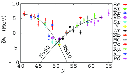
Figure 1: (Color online) Systematics for the shell correction used in the Fermi gas description of the level density. See text for details.

The systematics for the average total s-wave radiation width were determined by assuming a simple dependence on the mass and s-wave resonance spacing:

$$\left\langle\Gamma_{\gamma}\right\rangle_{0}^{\mathrm{sys}}=\left[aA+b\right]\left[c\log_{10}\left(D_{0}\right)+d\right].$$ (11)

Making a least-squares fit to measured $\left\langle\Gamma_{\gamma}\right\rangle_{0}$ (in meV) and $D_{0}$ (in keV) taken from the compilations of Belgya et al. (2005) yields the coefficients $a=-5.928$, $b=343.8$, $c=-42.43$, and $d=343.8$. These systematics were then used to generate a list of suggested values of $\left\langle\Gamma_{\gamma}\right\rangle_{0}$ for nuclei in the range $34\leq Z\leq 46$. The list includes the available experimental values. Systematic values were chosen based on measured $D_{0}$ where available, or on values of $D_{0}$ calculated from the regional level density systematic shown in Fig. 1. The line shape of the E1 photon strength function is described using a simplified version of the extended generalized Lorentzian (EGLO) model Kopecky et al. (1993). The EGLO model corresponds to a Lorentzian with an energy-dependent width. We are using a simplified version in which the width is set to depend only on the nuclear temperature at the energy of the decaying state and not on the energy of the final state. The most important feature, however, is that the magnitude of the strength function is normalized to reproduce the average total s-wave radiation width.

Since we are interested in modeling reactions for a relatively large region of isotopes we use the global nucleon-nucleus optical-model potential by Koning and Delaroche Koning and Delaroche (2003) for the calculations of the nucleon transmission coefficients. It has been shown Koning and Delaroche (2003) that this parameterization gives a very satisfactory fit to measured total cross section data and low-energy observables, such as the s-wave strength function, that are relevant for our application.

IV.2 Neutron capture cross sections for Zr isotopes

Our calculated $(n,\gamma)$ cross sections for the selected range of Zr isotopes ^90-95Zr are shown in Fig. 2. The experimental data for the quantities that constrained our decay model is summarized in Table 1. As noted earlier, the two most important ones are the average total s-wave radiation width, $\left<\Gamma_{\gamma}\right>_{0}$, and the measured s-wave resonance spacing, $D_{0}$. For the two radioactive isotopes, ⁹³Zr and ⁹⁵Zr, for which no such experimental data exist, we have used values obtained from the regional systematics described in the previous section. The error bars given for these cases are estimates based on typical experimental uncertainties for other isotopes in this region. Error estimates for our calculated $(n,\gamma)$ cross sections are shown as dashed and dash-dotted lines in Fig. 2. They were obtained by repeating the calculations using the upper and lower limits of the s-wave radiation width and level spacing, respectively. Our calculated results are compared to available experimental data from the EXFOR/CSISRS database Macklin et al. (1963); Kapchigashev (1965); Boldeman et al. (1975); Musgrove et al. (1977); K.Ohgama et al. (2005); Boldeman et al. (1976); Macklin (1985); Wyrick and Poenitz (1982); Lyon and Macklin (1959) and we find a satisfactory agreement for the isotopes that are well studied and are characterized by high level densities, which implies that the statistical-reaction treatment is well justified. However, the resonance spacing in ⁹¹Zr is rather large and signatures of individual peaks are observed in the ${}^{90}{\text{Zr}}(n,\gamma){}^{91}{\text{Zr}}$ experimental data which suggests that the statistical treatment might not be appropriate for this case. In Table 1 we also present the Maxwellian-averaged $(n,\gamma)$ cross section (MACS) at $k_{B}T=30$ keV. Our results are compared to values recommended by Z.Y. Bao et al. Bao et al. (2000), which are based on an evaluation of available experimental and theoretical results.

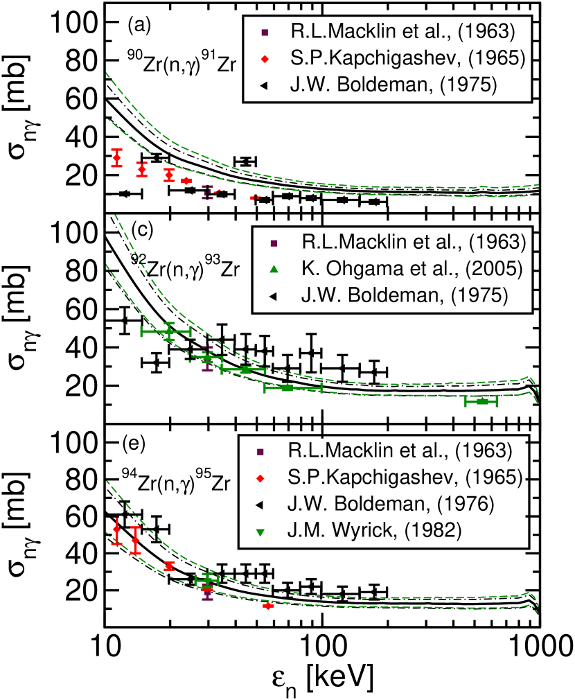
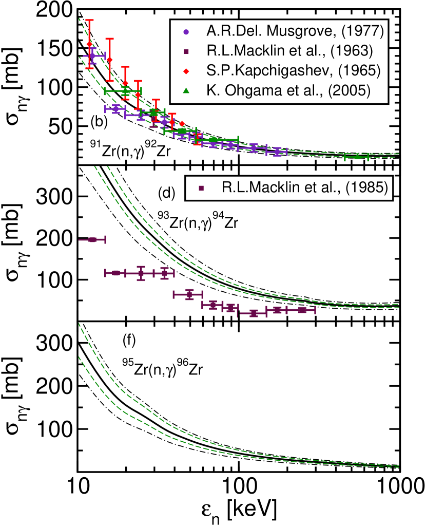
Figure 2: (Color online) Calculated $(n,\gamma)$ cross sections compared to experimental data for six Zr isotopes: ⁹⁰Zr, ⁹¹Zr, ⁹²Zr, ⁹³Zr, ⁹⁴Zr, and ⁹⁵Zr. Experimental data are from Refs. Macklin et al. (1963); Kapchigashev (1965); Boldeman et al. (1975); Musgrove et al. (1977); K.Ohgama et al. (2005); Boldeman et al. (1976); Macklin (1985); Wyrick and Poenitz (1982); Lyon and Macklin (1959). Dashed and dash-dotted lines indicate error bars associated with uncertainties in the s-wave resonance spacing $D_{0}$ and the s-wave average radiative width $\langle\Gamma_{\gamma}\rangle_{0}$, respectively. The error bars for the ⁹³Zr and ⁹⁵Zr $(n,\gamma)$ reactions are estimates based on typical experimental uncertainties for other isotopes in this region.

Table 1: Maxwellian-averaged $(n,\gamma)$ cross section at thermal energy $k_{B}T=30$ keV calculated for different Zr targets. The results from this work are compared to the recommended values by Z.Y. Bao et al. Bao et al. (2000). Also shown in the table are: $Q$ ($Q$-value for the reaction), $N_{D}$ (number of known discrete states in the compound nucleus that form a complete spectrum), $U_{m}$ (matching energy of constant temperature and Fermi-gas level-density regions), $D_{0}$ (level spacing for $s$-wave resonances at the neutron separation energy), and $\left\langle\Gamma_{\gamma}\right\rangle_{0}$ ($s$-wave average radiative width). Experimental data are from the RIPL-2 database Belgya et al. (2005), whereas unmeasured quantities are obtained from our regional systematics.

	90Zr$(n,\gamma)$	91Zr$(n,\gamma)$	92Zr$(n,\gamma)$	93Zr$(n,\gamma)$	94Zr$(n,\gamma)$	95Zr$(n,\gamma)$
$Q$ [MeV]	7.194	8.635	6.734	8.221	6.462	7.856
$N_{D}$	41	6	3	9	1	8
$U_{m}$ [MeV]	3.167	4.658	2.054	3.058	2.0	2.695
$D_{0}$ [keV]	$6.0\pm 1.4$	$0.55\pm 0.10$	$3.5\pm 0.8$	$0.160\pm 0.015$	$3.2\pm 0.8$	$0.26\pm 0.04$
$\left\langle\Gamma_{\gamma}\right\rangle_{0}$ [meV]	$130\pm 20$	$140\pm 40$	$135\pm 25$	$164\pm 40$	$85\pm 20$	$144\pm 40$
Maxwellian-averaged $(n,\gamma)$ cross section (in mb) at thermal energy $k_{B}T=30$ keV
This work	$26\pm 7$	$62\pm 19$	$41\pm 11$	$198\pm 44$	$27\pm 9$	$117\pm 34$
Bao et al. Bao et al. (2000)	$21\pm 2$	$60\pm 8$	$33\pm 4$	$95\pm 10$	$26\pm 1$	$79\pm 12$

Table 2: A summary of the decay models for ⁹¹Zr$(n,\gamma)$⁹²Zr  that are used in this work to investigate the sensitivity to certain key quantities.

	$\left\langle\Gamma_{\gamma}\right\rangle_{0}$	$D_{0}$	$\delta W$	MACS at
	[meV]	[keV]	[MeV]	30 keV [mb]
Reference	140	0.55	-1.743	62
Decay model 1	280	0.55	-1.743	115
Decay model 2	140	0.45	-1.237	74

V Theoretical analysis of decay data from a surrogate experiment

In this section we explore different approaches for utilizing decay probabilities measured in a surrogate experiment to extract low-energy neutron capture cross sections. We perform our simulations for the ⁹¹Zr$(n,\gamma)$⁹²Zr reaction. Let us first take a closer look at some of the details of the statistical-reaction calculation introduced in the previous section. The decay model for ⁹²Zr described in Sec. IV.1 will act as our reference model for these studies, and the corresponding $(n,\gamma)$ cross section serves as the reference (or “true”) cross section that we seek to extract from our simulated surrogate experiments.

V.1 The ⁹¹Zr$(n,\gamma)$⁹²Zr reaction

Neutron transmission coefficients calculated with the global optical-model potential by Koning and Delaroche Koning and Delaroche (2003) are shown in Fig. 3(a) for several partial waves on a ⁹¹Zr target. For $l>0,$ these are the appropriately weighted averages of the coefficients with $j=l\pm\frac{1}{2}$. The rapid increase of the p-wave transmission coefficient with increasing neutron energy is characteristic of all isotopes in this mass region, and corresponds to the well known $3p$ giant single-particle resonance. An interesting consequence of this feature is that low-energy neutron absorption (above approximately 10 keV) populates predominantly the $J\Pi$-states of the compound nucleus that can be reached by either s-wave or p-wave capture. The effect is clearly illustrated in Fig. 3(b) where the $J\Pi$ population of ⁹²Zr, following the absorption of 30 keV neutrons on ${}^{91}{\text{Zr}}(5/2^{+})$, is shown to be dominated by $1^{-},2^{-},3^{-},4^{-}$ and $2^{+},3^{+}$ states.

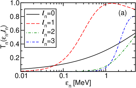
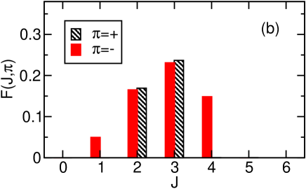
Figure 3: (Color online) (a) Energy- and $l$-dependence of neutron transmission coefficients on a ⁹¹Zr target. (b) $J\Pi$ population of the ⁹²Zr compound nucleus following neutron absorption on ${}^{91}{\text{Zr}}(5/2^{+})$ at $\varepsilon_{n}=30$ keV.

It is important to realize that there is generally a very small number of open decay channels following the absorption of low-energy neutrons on spherical, or near-spherical, targets. Other particle-decay thresholds usually appear above the neutron separation energy, and inelastic channels are closed when the first excited states of the target are above the incoming neutron energy. This leaves only two possible decay paths: compound-elastic scattering leading back to the target ground state, and gamma deexcitation of the compound nucleus. We now focus on the branching ratio defined in Eq. (2). In this special case, the sum over open channels ($\chi^{\prime}$) appearing in the denominator contains only two terms. The important quantities are therefore the neutron transmission coefficients discussed above and the product of the gamma transmission coefficients with the level density of the compound nucleus. The latter quantity must be integrated over all states that can be reached by a primary gamma transition. For low-energy neutrons, a single gamma deexcitation is usually enough to bring the compound nucleus below the neutron-decay threshold, which will inevitably lead to a continued gamma cascade down towards the ground state. As noted previously, the Stapre code correctly computes the gamma cascade even when neutron emission is possible within the cascade.

Fig. 4 shows the gamma branching ratios for ⁹²Zr as a function of $J\Pi$ and neutron energy. For comparison we also plot the total gamma decay probability which we define as the ⁹²Zr production cross section divided by the neutron absorption cross section. These results are obtained with width-fluctuation corrections turned off. The results shown in this plot demonstrate a feature of nuclei that is particularly striking near closed shells, namely a dramatic dependence of the compound-nucleus gamma decay branching ratios on $J\Pi$ at low energies above threshold. For some $J\Pi$ values the probability for gamma decay is close to one, whereas for others it is on the order of $10^{-3}$. Clearly we are very far from the Weisskopf-Ewing limit and certain approximations that have previously been used in the analysis of surrogate experiments cannot be used here. The reason for the dramatic dependence on $J\Pi$ is the behavior of the neutron transmission coefficients, shown in Fig. 3(a), in combination with the small number of discrete states at low excitation energies in the initial nucleus ⁹¹Zr. Those compound-nuclear states in ⁹²Zr that can reach an energetically allowed state in ⁹¹Zr by the emission of an s- or p-wave neutron have a very small gamma-decay probability. For the other states, the branching ratios are determined by the competition between $l\geq 2$ neutron transmission coefficients and gamma transmission coefficients. It turns out that the gamma-decay channel usually dominates although the gamma transmission coefficients are still very small. It is also important to note the convergence of the curves at higher energies $E_{n}\gtrsim 3$ MeV. This demonstrates the onset of the Weisskopf-Ewing limit with the resulting approximate independence of $J\Pi$ for the branching ratios. In the Sec. V.3 we return to this issue and discuss how we can utilize the observed behavior for our purposes.

Before we discuss the sensitivity to properties of the nuclear decay model, we introduce the notation $\sigma^{\mathrm{ref}}_{n\gamma}(\varepsilon_{n})$, $\sigma^{\mathrm{ref}}_{\mathrm{abs}}(\varepsilon_{n})$, and $G^{\mathrm{ref}}_{\gamma}(U,J,\Pi)$. These quantities are the results of our reference calculation and they denote, respectively, the radiative neutron-capture cross section, the neutron absorption cross section, and the gamma branching ratios of Eq. (1).

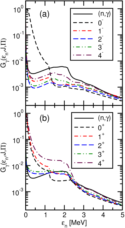
Figure 4: (Color online) Gamma branching ratios as a function of spin, parity and excitation energy of the decaying state in ⁹²Zr. The energy is given as the equivalent neutron energy $\varepsilon_{n}=U-S_{n}$. The total gamma-decay probability following neutron absorption, as described in the text, is shown as a solid line in both panels. Width-fluctuation corrections were turned off when producing these results.

By introducing variations from the reference decay model we will be able to study the effects of our lack of knowledge of the true decay model, which is one of the two major uncertainties associated with the surrogate method. As previously mentioned, the modeling of neutron capture reactions is most sensitive to the nuclear level density at, and somewhat below, the neutron separation energy, as well as to the E1 photon strength function at small gamma energies ($\sim 2-3$ MeV). In order to quantitatively investigate this sensitivity we introduce two decay models, “Decay model 1” and “Decay model 2”, in addition to the “Reference Decay model” corresponding to the parameter set from the regional systematics. The most important parameters for the three models are summarized in Table 2, together with the resulting MACS at 30 keV. The salient feature of Decay model 1 is a factor of two increase in the magnitude of the E1 photon strength function. Such uncertainty in the size of the gamma-transition strength is not unrealistic when moving to unstable isotopes for which no experimental data exists. The $(n,\gamma)$ cross section is almost directly proportional to the magnitude of the E1 photon strength function, as is clearly seen in Fig. 5 where the ratio of the modeled capture cross section to the reference calculation is shown. The logarithmic energy axis was introduced in order to cover a large energy range while still focusing on the relevant small energies. For Decay model 2 we decreased the level spacing $D_{0}$ for s-wave resonances by modifying the shell correction $\delta W$ in the formula for the level-density parameter $a$, Eq. (LABEL:eq:ilj-apar). We choose this particular way of modifying the level density since $\delta W$ is the free parameter in our regional systematic. The $\lesssim 20$% decrease of the level spacing at the separation energy implies a $\gtrsim 20$% increase of the level density, and again we observe a proportional increase in the capture cross section. Finally, we present the results obtained when turning off the width-fluctuation corrections. As expected, turning off width-fluctuation corrections results in an increase in the capture cross section. From Fig. 5 we infer that it is approximately a 10% effect at small energies and completely negligible at higher energies ($\gtrsim 2$ MeV).

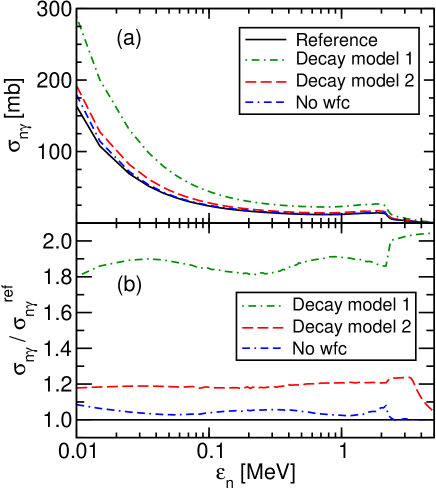
Figure 5: (Color online) Sensitivity of the ⁹¹Zr$(n,\gamma)$⁹²Zr cross section to variations of key parameters in the decay model. (a) Cross sections calculated using the three decay models of Table 2 plus one calculation using the Reference Decay model but turning off width-fluctuation corrections. (b) The ratio to the reference cross section.

V.2 Simulating the direct reaction of a surrogate experiment

The first step of the reaction that takes place in a surrogate experiment is a direct reaction, such as a transfer or inelastic scattering reaction, that produces the relevant intermediate nucleus in a highly excited state. For the purpose of measuring the decay probabilities that are pertinent for the desired reaction, it is important that the intermediate nucleus first equilibrates into a compound-nuclear state. The relevant net result is therefore the distribution of $J\Pi$ states in the compound nucleus that is populated following the direct reaction. In principle, one would like to be able to describe this direct-reaction process, leading to an equilibrated compound nucleus, using an appropriate direct-reaction model. However, this is a non-trivial task since it requires a description of transfer and inelastic scattering reactions leading to unbound states, as well as an understanding of the damping of those states into equilibrated compound-nuclear states. Moreover, a variety of projectile-target combinations with a range of possible incident energies may be considered for producing the compound nucleus of interest. Different reaction mechanisms, regions of the nuclear chart, and projectile energies yield different compound-nuclear $J\Pi$ distributions and also provide different challenges for a proper theoretical description. DWBA calculations relevant to the present work for inelastic alpha scattering to highly excited states in spherical nuclei are currently under way and will be reported elsewhere.

For the present purpose of simulating surrogate experiments we use simple schematic distributions. Furthermore, we assume that the distributions are independent of the compound nucleus excitation energy in the energy range just above the neutron separation energy that we are interested in. Since inelastic scattering reactions can be used to populate most compound nuclei that are relevant for studies of s-process branch points, we employ distributions that exhibit the asymmetry between natural- and unnatural-parity states that is characteristic for those reactions with even-even targets. In the absence of a spin-dependent interaction, a distorted-wave Born approximation description of such a reaction yields only $J^{\Pi}=0^{+},1^{-},2^{+},3^{-},\ldots$ states. Distribution A, shown in Fig. 6(a), contains only such natural-parity states and we will use this distribution as the reference (“true”) population of the compound nucleus ⁹²Zr^∗ in a simulation of our benchmark surrogate reaction ${}^{92}{\text{Zr}}(\alpha,\alpha^{\prime}){}^{92}{\text{Zr}}^{*}$. For this reason we denote this distribution $F^{A,\mathrm{ref}}(J,\Pi)$. Furthermore, the gamma-decay probability that is obtained when combining this $J\Pi$ distribution with our reference gamma branching ratio, $G^{\mathrm{ref}}_{\gamma}(U,J,\Pi)$, in Eq. (5) will be denoted $P^{\mathrm{ref}}_{\gamma}(U)$. The decay probability $P^{\mathrm{ref}}_{\gamma}(U)$ thus corresponds to what would be measured in our simulated surrogate experiment, indicated as a solid curve in Fig. 9(a).

In addition to $F^{A,\mathrm{ref}}(J,\Pi)$ we use two more schematic distributions: $F^{A+\delta}(J,\Pi)$ and $F^{B}(J,\Pi)$. They are shown in Fig. 6(b,c), respectively. The first one is almost identical to $F^{A,\mathrm{ref}}(J,\Pi)$, but contains a small random noise to simulate a minor error in the predicted distribution. Finally, Distribution B represents a significantly different population without any asymmetry between different parity states. The average angular momentum deposited in the compound nucleus, $\langle J\rangle$, is approximately 2.0 for all distributions. Therefore, these simulations correspond to a study of the sensitivity to deviations in the assumed $J\Pi$ distribution while keeping the average transferred angular momentum approximately fixed.

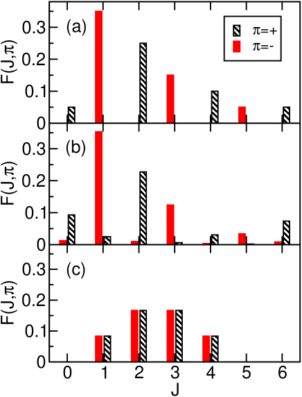
Figure 6: (Color online) Schematic surrogate populations used in this study: (a) $F^{A,\mathrm{ref}}(J,\Pi)$; (b) $F^{A+\delta}(J,\Pi)$; (c) $F^{B}(J,\Pi)$. See text for further details.

V.3 Three alternative analysis approaches

In the following we will assume that Distribution A, $F^{A,\mathrm{ref}}(J,\Pi)$, is a reasonable representation of the $J\Pi$ distribution of a compound nucleus created in a surrogate reaction (such as inelastic scattering off an even-even near-spherical nucleus). Also, we assume that the Reference Decay model with the parameters from Section IV represents a realistic description of the “true” decay of the compound nucleus, populated either through the neutron-induced or the surrogate reaction. The function $P_{\gamma}^{\mathrm{ref}}(U)$, calculated from Eq. (5) using the (energy-independent) formation probability $F(J,\Pi)$ from Distribution A and the branching ratios $G_{\chi}(U,J,\Pi)$ from the Reference Decay model, is then the quantity that is observed in our simulated Surrogate experiment. We now investigate various possibilities of extracting the desired “true” cross section $\sigma_{n\gamma}^{\mathrm{ref}}(\varepsilon_{n})$, represented by the “Reference” cross section in Fig. 5. In order to test the different procedures, we introduce uncertainties in the modeling by using Decay model 1 or 2 (see Table 2). This will illustrate the effect of having insufficient knowledge of the “true” decay of the compound nucleus. Furthermore, for the approaches that require the theoretical prediction of the $J\Pi$ population of the compound nucleus created in the surrogate reaction we make use of the schematic distributions introduced in Sec. V.2. This will illustrate the effect of having insufficient knowledge of the $J\Pi$ distribution of the decaying nucleus.

We discuss three different approaches that utilize decay data from a surrogate experiment to extract the desired low-energy $(n,\gamma)$ cross section. The three approaches are labeled as follows:

1. Weisskopf-Ewing approximation.

2. Full modeling of the $J\Pi$ population following the surrogate reaction.

3. Normalization of the decay model in the Weisskopf-Ewing region.

Below we discuss each one of these approaches in some detail and draw some conclusions regarding their applicability.

V.3.1 Weisskopf-Ewing approximation

The results and discussion of the preceding sections imply that the convenient Weisskopf-Ewing approximation cannot be utilized in the surrogate approach when trying to extract low-energy $(n,\gamma)$ cross sections for spherical and near-spherical targets. It was shown that the gamma-decay branching ratios depend very sensitively on the particular $J\Pi$ population of the intermediate nucleus due to the small number of open decay channels.

Fig. 7 illustrates the inadequacy of the Weisskopf-Ewing approximation for this purpose. In this simulation the extracted $(n,\gamma)$ cross section is obtained by simply multiplying the reference absorption cross section [$\sigma^{\mathrm{ref}}_{\mathrm{abs}}(\varepsilon_{n})$] by the reference surrogate decay data, [$P^{\mathrm{ref}}_{\gamma}(U)$]. This procedure corresponds to the simulation labeled “WE” in Table 3. The extracted cross section is compared to the reference cross section. We find disagreement at the level of one order of magnitude, and also that the shape of the extracted cross section is wrong.

Table 3: Combinations of decay models (see Table 2) and $J\Pi$ distributions (see Fig. 6) used in the simulations.

Simulation	Decay model	$J\Pi$ distribution
Reference	Reference	A,ref
WE	Reference	—
1	2	A+$\delta$
2	2	B
3	1	A+$\delta$
4	1	B

We briefly mention here the surrogate ratio method, which is based on the Weisskopf-Ewing approximation. This method has been used to extract $(n,f)$ cross sections in the actinide region Burke et al. (2006); Plettner et al. (2005). The goal of the ratio method is to determine the ratio of two cross sections of two “similar” compound-nuclear reactions. An independent determination of one of these cross sections then allows one to infer the other. The desired ratio of the two cross sections is obtained indirectly from surrogate measurements of the ratio of decay probabilities under the assumption that the Weisskopf-Ewing limit is valid. It was demonstrated in Ref. Escher and Dietrich (2006) that the ratio approach may actually reduce the error that is usually associated with neglecting the $J\Pi$ dependence of the branching ratios. However, as we have just shown in Fig. 7, the error encountered when applying the simple Weisskopf-Ewing approximation to low-energy $(n,\gamma)$ reactions is about one order of magnitude larger than in the $(n,f)$ case. In the latter case, the error rarely exceeds a factor of two even at small neutron energies (see in particular Fig. 10 of Ref. Escher and Dietrich (2006)). Furthermore, for spherical or near-spherical targets, the $J\Pi$ dependence of the gamma-decay branching ratios at low energies is very sensitive to the particular level structure of the target, as shown in Sec. IV. Thus, it is hard to reduce the effects of this sensitivity simply by measuring the ratio of decay probabilities for two neighboring isotopes.

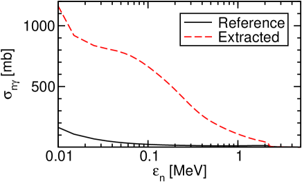
Figure 7: (Color online) Extraction of $(n,\gamma)$ cross section from a surrogate experiment simulation using the Weisskopf-Ewing approximation; see simulation “WE” of Table 3 and discussion in text.

V.3.2 Full modeling of the $J\Pi$ population following the surrogate reaction

For applications in the actinide region there have been attempts to take the effects of the $J\Pi$ population mismatch into account when estimating $(n,f)$ cross sections from surrogate experiment data Younes and Britt (2003a, b). In that work, the population of the compound nucleus following a $(t,p)$ reaction was calculated in a distorted-wave Born Approximation approach. Furthermore, efforts are currently underway to develop a more advanced direct-reaction framework in which the surrogate reactions to unbound states, and their subsequent equilibration into compound-nuclear states, can be studied in greater detail. However, the application of the surrogate method to low-energy $(n,\gamma)$ reactions is very challenging, in particular when near-spherical targets are involved. We will show that a small uncertainty in the predicted $J\Pi$ population can lead to a very large error in the extracted cross section.

A surrogate analysis inspired by the diagram depicted in Eq. (6) is performed by first introducing a modeled gamma-decay probability, $P_{\gamma}^{\mathrm{model}}(U)$, with both the $J\Pi$ distribution and the gamma-decay branching ratios obtained from initial modeling efforts

$$\begin{split}P_{\gamma}^{\mathrm{model}}(U)&=\sum_{J,\Pi}F^{\mathrm{model}}(U,J,\Pi)G_{\gamma}^{\mathrm{model}}(U,J,\Pi)\\ &\equiv\sum_{J,\Pi}P_{\gamma}^{\mathrm{model}}(U,J,\Pi).\end{split}$$ (12)

This calculated quantity is then compared to the measured gamma-decay probability. A fit to the experimental data is achieved by introducing a fitting function $\eta(U,J,\Pi)$ that relates the modeled decay probability with the measured one

$$P_{\gamma}^{\mathrm{exp}}(U)=\sum_{J,\Pi}\eta(U,J,\Pi)P_{\gamma}^{\mathrm{model}}(U,J,\Pi).$$ (13)

For simplicity we assume that the functions $\eta(U,J,\Pi)$ are independent of $J$ and $\Pi$ so that the fit corresponds to an energy-dependent normalization. In this case it is simple to evaluate the correction factor as

$$\eta(U)=\frac{P_{\gamma}^{\mathrm{exp}}(U)}{P_{\gamma}^{\mathrm{model}}(U)},$$ (14)

and subsequently use it to extract the desired cross section

$$\begin{split}\sigma^{\mathrm{extract}}_{n\gamma}(\varepsilon_{n})=\eta(U)&\sum_{J,\Pi}\sigma^{\mathrm{model}}_{\mathrm{abs}}(\varepsilon_{n},J,\Pi)\\ &\quad\times G^{\mathrm{model}}_{\gamma}(U,J,\Pi)w_{n\gamma}(\varepsilon_{n},J,\Pi).\end{split}$$ (15)

In the final step we have also introduced the theoretical width-fluctuation corrections, $w_{n\gamma}(\varepsilon_{n},J,\Pi)$. The numerical calculations discussed below were calculated using the statistical-model code Stapre to calculate the various factors in the above equation, including the width-fluctuation corrections, $w_{n\gamma}(\varepsilon_{n},J,\Pi)$.

We will now test this procedure by performing several simulations. We use the simulated surrogate decay data, $P_{\gamma}^{\mathrm{ref}}(U)$, as corresponding to the experimental data in the numerator of Eq. (14). As for the calculated quantity appearing in the denominator, we introduce some variations in the modeled decay probabilities and the predicted $J\Pi$ population. The question is to what extent the analysis procedure will be able to correct for these variations. In the first simulation we use Decay model 2 to calculate $G_{\gamma}^{\mathrm{model}}(U,J,\Pi)$. We know that this decay model overestimates the cross section by $\sim$20 % (see Table 2). Furthermore, we assume that we have a very good, but not perfect, estimate of the $J\Pi$ population of the intermediate nucleus. The distribution $F^{\mathrm{model}}(U,J,\Pi)$ only differs from the reference (“true”) population $F^{A,\mathrm{ref}}(J,\Pi)$ by a small random noise. For this purpose we use the distribution $F^{A+\delta}(J,\Pi)$ shown in Fig. 6(b). The combination of Decay model 2 and the $J\Pi$ distribution $F^{A+\delta}(J,\Pi)$ is denoted Simulation 1 in Table 3. The procedure outlined above results in the normalization function $\eta(U)$, shown in Fig. 8(b) plotted as a function of the equivalent neutron energy $\varepsilon_{n}$. Using this normalization function in Eq. (15) yields the extracted $(n,\gamma)$ cross section shown as a dashed line in Fig. 8(a). For this case the procedure works relatively well and the MACS at 30 keV for the extracted cross section is 67 mb. This number should be compared with the 74 mb that is the original prediction of Decay model 2, and the 62 mb that is the reference result that we were aiming for.

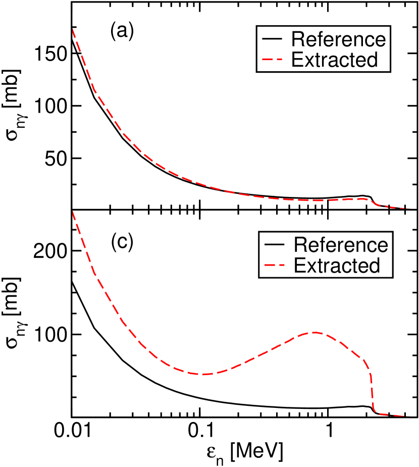
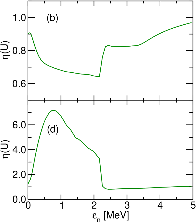
Figure 8: (Color online) Extraction of $(n,\gamma)$ cross section from two different surrogate experiment simulations using a full modeling of the $J\Pi$ population: (a) Simulation 1, and (c) Simulation 2, see Table 3. Panels (b) and (d) show the respective normalization functions $\eta(U)$. Note that $U=\varepsilon_{n}+S_{n}$.

In the second simulation we use a model for the $J\Pi$ population that is a poor representation of the “true” $J\Pi$ distribution. In this case, we find that the approach outlined above results in a very poor correction of the decay model, and consequently of the extracted cross section. For this simulation we use the combination of Decay model 2 and the $J\Pi$ distribution $F^{B}(J,\Pi)$, which is denoted Simulation 2 in Table 3. The extracted $(n,\gamma)$ cross section is shown as a dashed line in Fig. 8(c), and the normalization function $\eta(U)$ is shown in Fig. 8(d). The extracted cross section is very different from the desired result below about 2.2 MeV.

The above results imply that one may be able to use surrogate data to correct a theoretical decay model provided one has sufficiently accurate information on the $J\Pi$ population of the compound nucleus that decays in the surrogate experiment. Obtaining a reliable prediction of the relevant $J\Pi$ population is challenging, since it requires accurate direct-reaction calculations involving the nuclear continuum. Furthermore, the equilibration process that follows the production of a highly excited, intermediate nucleus in a surrogate reaction is not sufficiently well understood; possible decay mechanisms other than damping into the compound nucleus need to be accounted for if they are present. Nevertheless, it may be possible to obtain some experimental signatures of the $J\Pi$ population of the decaying nucleus. While the high sensitivity of the gamma-decay branching ratios to the $J\Pi$ population makes the extraction of the desired cross section from a surrogate experiment very difficult, it should also result in certain experimental observables, such as the relative intensities of discrete gamma transitions, being useful to constrain calculated $J\Pi$ distributions. This remains to be investigated in more detail.

V.3.3 Normalization of the decay model in the Weisskopf-Ewing region

In the third approach we utilize the fact that surrogate experiments can, in principle, provide decay data for a very wide energy range. Thus it is possible to collect data from an energy region in which the Weisskopf-Ewing limit is approximately correct. For ⁹²Zr, we find from Fig. 4, that this occurs at $\varepsilon_{n}$ approximately 3 MeV. A fit to the surrogate decay data in this region will be less sensitive to the predicted $J\Pi$ population than at lower energies. In addition, the sensitivity studies for the calculated $(n,\gamma)$ cross section, presented in Sec. V.1, showed that modeling errors in the s-wave average radiative width $\left\langle\Gamma_{\gamma}\right\rangle_{0}$, or in the level spacing $D_{0}$, change primarily the magnitude of the calculated cross section, but do not affect the energy dependence of the cross section very much. Therefore, one may try to normalize the decay model in the Weisskopf-Ewing region, where the modeled quantities are not very sensitive to the $J\Pi$ population. The extracted scaling factor is then used in the final calculation of the desired cross section at small energies. The normalization simply becomes an energy- and $J\Pi$-independent factor, $\eta$.

We examine the outcome of this approach for three different simulations. As before, we employ the decay probability $P^{\mathrm{ref}}_{\gamma}(U)$ to represent the measured quantity in our simulated surrogate experiment. It is shown as a solid line in Fig. 9(a). The dashed line corresponds to the modeled decay probability obtained from Simulation 2, see Table 3, using the schematic distribution B (representing a large error compared to the reference “true” distribution), combined with Decay model 2 (yielding gamma-decay branching ratios that are overestimated by $\sim$20%). The dash-dotted line is the modeled decay probability of Simulation 3, in which the schematic distribution $F^{A+\delta}(J,\Pi)$ is used in combination with Decay model 1. In this case, the modeled $J\Pi$ population is very close to the reference distribution, but the decay model is one that produces gamma-decay branching ratios that are known to be a factor two too large. The dash-dash-dotted line corresponds to Simulation 4 in which we still use Decay model 1, but the population of the intermediate state is described by the schematic distribution B. From Fig. 9(a) we observe that the calculated gamma-decay probabilities differ by up to an order of magnitude in the most relevant energy regime.

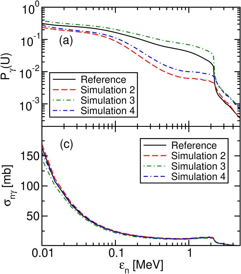
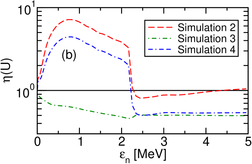
Figure 9: (Color online) (a) Gamma-decay probabilities for different simulations. The solid line corresponds to the reference model whereas the other three are based on different combinations of the assumed $J\Pi$ population and decay model (see Table 3). (b) The normalization functions $\eta(U)$. Their value at $\varepsilon_{n}=3$ MeV is used in the final cross section calculation. Note that $U=\varepsilon_{n}+S_{n}$. (c) The extracted cross sections, for the respective simulations, obtained by employing the analysis approach outlined in Sec. V.3.3. The solid line is the reference cross section.

The next step in the analysis procedure is to construct the normalization functions $\eta(U)$ as described in Eq. (14). The resulting functions are shown in Fig. 9(b). In this analysis approach, we focus on the high-energy region in which the normalization functions have become almost energy-independent. This is the region in which the Weisskopf-Ewing limit is approximately applicable. Still, we want to extract the normalization at an energy which is not too far away from the region of interest. In this particular case we use the energy $\varepsilon_{n}=3$ MeV, and for our three different simulations we obtain the normalization factors $\eta=$ 0.88, 0.50, and 0.54, respectively. The final step is simply to apply this constant renormalization to our modeling of the desired reaction in Eq. (15). Again, we introduce width fluctuation corrections at this stage. Note that a different decay model was used in Simulation 2 as compared to Simulations 3 and 4, and that both of them differ from the reference (“true”) decay model. The final result of this procedure is shown in Fig. 9(c) where the extracted cross sections are compared to the reference result represented by the solid line. The quality of the extracted cross sections is remarkable considering the very different initial choices of decay models and $J\Pi$ populations. The MACS at 30 keV for the three simulations are 65, 58, and 62 mb, respectively, to be compared to the 62 mb for the reference cross section.

The underlying reason for the success of this approach is the direct proportionality between variations of the level density formula, or gamma-strength function, and the corresponding effect on the gamma-decay branching ratios as demonstrated, e.g., in Fig. 5. In the Weisskopf-Ewing limit this proportionality leads to a universal and energy-independent scaling of all $J\Pi$ components. This observation promises to be very useful for surrogate experiments in which data can be obtained for equivalent neutron energies at which the Weisskopf-Ewing limit is applicable. However, as we have seen in the ⁹²Zr example, see Fig. 9(a), the surrogate gamma-decay probabilities are quite small for energies above $\varepsilon_{n}\sim 1$ MeV, and consequently the measurement is challenging. The conclusion is that, given good-quality surrogate data in this energy region, the normalization approach outlined above offers an almost model-independent way of extracting the low-energy $(n,\gamma)$ cross section for spherical and near-spherical nuclei.

VI Conclusions and recommendations

We have examined the feasibility of using the surrogate method to extract low-energy $(n,\gamma)$ cross sections for spherical and near-spherical nuclei in the mass 90-100 region. In particular, several Zr isotopes were studied and the ⁹¹Zr$(n,\gamma)$⁹²Zr reaction was used as a test case. Our study was performed by carrying out simulations to explore three different approaches to utilize surrogate reaction data. The sensitivity of the extracted cross sections to uncertainties in the theoretical modeling was investigated for the different approaches and their performance was assessed by comparing with a predetermined benchmark.

One of the main results of the paper is the demonstration of the large sensitivity of the gamma-decay branching ratios, and consequently the surrogate-reaction gamma-decay probability, to the $J\Pi$ population of the intermediate compound nucleus, and the effect that this sensitivity has on the extracted cross section. It was found that an approach in which the $J\Pi$ population mismatch was not taken into account, gave an extracted cross section that deviated from the benchmark result by an order of magnitude. On the other hand, full modeling of the population of the compound nucleus is very difficult as it involves the description of direct reactions to continuum states and their subsequent equilibration into a compound-nuclear state. The third and final analysis approach proposed in this paper promises to be the most viable one. It begins with a careful modeling of the decay, preferably using regional systematics to constrain unknown nuclear properties. Surrogate decay data collected at slightly higher energies are then utilized to normalize the modeled gamma-decay branching ratios so that the desired cross section can be extracted.

It needs to be emphasized that these findings, and the sensitivities that were studied, apply to the analysis of our simulated surrogate experiment. In actual experiments, additional uncertainties are introduced, e.g., the identification of the final state, and the finite energy and angular resolutions. Furthermore, a prerequisite for our simulations of surrogate reactions has been the population of a fully equilibrated compound-nuclear intermediate state. The question how this state is formed, through the population of highly-excited states in the direct surrogate reaction followed by multi-step equilibration processes, deserves to be studied in much greater detail. In particular, the probability for pre-equilibrium emission of particles should be investigated for different surrogate reactions.

The theoretical modeling in this paper was performed using Hauser-Feshbach statistical-reaction theory. The approaches for normalizing the decay model using surrogate-reaction experimental data is based on the use of traditional decay models. Furthermore, these decay models were applied to describe the decay from all relevant $J\Pi$ states in the entire energy range of interest. This implies that the arguments presented here are not applicable to regions of nuclei that are too far away from the valley of stability, where the use of established level-density formulae and parameterized gamma-strength functions has to be questioned. The same observation applies to the optical potentials that were used in this work to calculate particle transmission coefficients. The normalization procedures outlined in Sec. V.3 rests on the accuracy of the optical model that is used to compute the absorption cross section. Finally, we stress that width fluctuation corrections were always applied in the final modeling part of the analysis. Those corrections cannot be obtained from the surrogate experimental data.

With the insights gained from this study we can give a few general recommendations for future surrogate experiments: (1) Good particle identification is very important since one needs the absolute normalization to get the decay probabilities with good accuracy. We note that the gamma-decay probability is expected to decrease dramatically in magnitude and one must be able to measure them up to a few MeV above the neutron separation energy. (2) Consequently one also needs to be able to efficiently identify the desired decay channel. For gamma decay this might require the existence of a very strong collector $2^{+}\rightarrow 0^{+}$ transition to tag the occurrence of a gamma cascade. This requirement would limit the method to cases where the intermediate nucleus is an even-even isotope. However, other options for tagging the gamma cascade are being considered Bernstein . (3) The energy resolution is less of an issue if the approach of renormalizing the decay model at high energies is used. In this procedure the energy dependence is obtained from the statistical-reaction modeling. Still, an energy resolution that is better than 100 keV should be desirable. (4) Additional experimental information, such as relative intensities of the gammas de-exciting low-lying levels of different spin and parity, can help to gain insight into the $J\Pi$ population of the compound nucleus. However, one should remember that the observed gamma intensities depend on the properties of the gamma cascade that proceeds through the quasi-continuum as well as on the initial $J\Pi$ distribution, and so it is important that the properties of this cascade be accurately modeled. (5) Measuring the decay at different emission angles of the ejectile in the initial direct reaction should provide an experimental handle to vary the $J\Pi$ population. However, it remains to be seen from direct-reaction modeling for each particular case how large this change can actually be. (6) Finally, we recommend that benchmark experiments, in which the surrogate data is used to extract a known cross section, are carried out since this will provide very valuable insights into the issues discussed in this paper.

Finally, we note that applications involving spherical nuclei probably constitute one of the most challenging applications of the surrogate method. This statement applies, in particular, to isotopes near magic shells such as the Zr isotopes studied in the present work. In addition, low-energy $(n,\gamma)$ reactions provide the most difficult reaction with regards to the angular momentum mismatch. In contrast, for deformed nuclei there is usually a larger number of open decay channels and that reduces the sensitivity of the gamma-decay branching ratios to the initial $J\Pi$ population. In particular, the Weisskopf-Ewing limit might be reached already at relatively low excitation energies above the neutron separation energy.