Nuclear forces with $\Delta$-excitations up to next-to-next-to-leading order I:
peripheral nucleon-nucleon waves

Abstract

We study the two-nucleon force at next-to-next-to-leading order in a chiral effective field theory with explicit $\Delta$ degrees of freedom. Fixing the appearing low-energy constants from a next-to-leading order calculation of pion-nucleon threshold parameters, we find an improved convergence of most peripheral nucleon-nucleon phases compared to the theory with pions and nucleons only. In the delta-full theory, the next-to-leading order corrections are dominant in most partial waves considered.

I Introduction

The forces between nucleons based on chiral effective field theory have been studied in great detail over the last decade, for reviews see e.g. Bedaque:2002mn ; Epelbaum:2005pn . Most calculations are based on the chiral effective Lagrangian formulated in terms of the asymptotically observed ground state fields, the pions and nucleons chirally coupled to external sources. The excitation of baryon and meson resonances is encoded in the low-energy constants (LECs) of the pion-nucleon interaction beyond leading order. Such a framework provides an accurate representation of the nucleon-nucleon (NN) phase shifts if extended to sufficient high order, state-of-the-art calculations have been carried out to next-to-next-to-next-to-leading order in the chiral expansion. This is very similar to the description of pion-nucleon scattering in chiral perturbation theory well below the $\Delta$-excitation energy, where a precise description of the pertinent phase shifts has been obtained in a complete one-loop (fourth order) calculation, see e.g. Ref. Fettes:2000xg . Still, it can be argued that the explicit inclusion of the delta, which is the most important resonance in nuclear physics, allows one to resum a certain class of important contributions and thus leads to an improved convergence as compared to the delta-less theory, provided a proper power counting scheme such as the small scale expansion (SSE) Hemmert:1997ye is employed. The SSE is a phenomenological extension of chiral perturbation theory in which the delta-nucleon mass splitting is counted as an additional small parameter. This improved convergence has been explicitely demonstrated for pion-nucleon scattering where the description of the phase shifts at third order in the SSE comes out superior (inferior) to the third (fourth) order chiral expansion in the pure pion-nucleon theory Fettes:2000bb . Note, however, that the theory with explicit deltas has more LECs at a given order due to the richer operator structure when spin-3/2 fields are present. Clearly, for a description of pion-nucleon scattering in the $\Delta$-region or pion production in NN collisions the inclusion of the spin-3/2 fields as active degrees of freedom is mandatory, see e.g. Hanhart:2003pg for a review.

In this work, we want to analyze the two-nucleon forces by systematically including the $\Delta$-resonance beyond leading order in the small scale expansion, extending earlier work presented in Refs. Ordonez:1995rz ; Kaiser:1998wa (the precise relation to these papers will be given below). More precisely, we construct and analyze the two-pion exchange NN potential at next-to-next-to-leading order (NNLO). For that, we must determine the sum of the subleading $\pi N\Delta$ LECs $b_{3},b_{8}$ together with the $\pi N$ LECs $c_{i}$ (the values of these differ from the ones obtained in chiral perturbation theory). This is achieved by working out the threshold coefficients of pion-nucleon scattering from tree graphs at second order which is of sufficient accuracy for the inclusion of the corresponding operators in the NNLO potential. From that, we can deduce the momentum and coordinate space representations of various isoscalar and isovector potentials. Having done that, we calculate the peripheral phases in NN scattering based on perturbation theory. It is well established that these peripheral waves do not require a non-perturbative resummation and therefore let one most directly analyze the effects of various contributions to the effective two-nucleon potential.

The manuscript is organized as follows. In Sect. II we work out the contributions of the two-pion exchange (TPE) graphs including the $\Delta$-resonance at NNLO. We then determine the corresponding dimension-two LECs from a fit to the $\pi N$ threshold parameters in Sect. III. The resulting coordinate space representation of the TPE potential and the peripheral NN waves are shown and discussed in Sect. IV. We end with a summary and outlook. The appendix contains explicit analytical formulae for the $\pi N$ threshold coefficients.

II $\Delta$-contributions to the two-nucleon force up to NNLO

In this chapter, we construct the two-pion exchange potential (TPEP) with one or two intermediate $\Delta$-state(s) at NNLO. We employ here standard Weinberg power counting for the two-nucleon effective potential, that is the leading TPEP starts at next-to-leading order (NLO) ($\nu=2$) and the first corrections to it appear at NNLO ($\nu=3$). The leading order ($\nu=0$) potential is given by the static one-pion exchange. Since we are only considering peripheral waves with the angular momentum $l\geq 2$, no four-nucleon contact interactions contribute to the accuracy we are working at.

II.1 Effective Lagrangian and power counting

The calculations performed in the following are based on the effective chiral Lagrangian of pions, nucleons and deltas. We employ here the heavy baryon formulation and display only the terms of relevance for our study:

$${\cal L} = {\cal L}^{(1)}+{\cal L}^{(2)}+\ldots$$

$${\cal L}^{(1)} = \bar{N}\,{\cal A}_{\pi N}^{(1)}\,N+\bar{T}\,{\cal A}_{\pi\Delta}^{(1)}\,T+\left(\bar{T}\,{\cal A}_{\pi N\Delta}^{(1)}\,N+{\rm h.c.}\right)~{},$$

$${\cal L}^{(2)} = \bar{N}\,{\cal A}_{\pi N}^{(2)}\,N+\left(\bar{T}\,{\cal A}_{\pi N\Delta}^{(2)}\,N+{\rm h.c.}\right)~{},$$ (2.1)

with

$${\cal A}_{\pi N}^{(1)} = i\,v\cdot D+g_{A}\,u\cdot S~{},$$

$${\cal A}_{\pi N}^{(2)} = c_{1}\,\langle\chi_{+}\rangle+c_{2}\,(v\cdot u)^{2}+c_{3}\,u\cdot u+c_{4}\,[S^{\mu},S^{\nu}]u_{\mu}u_{\nu}~{},$$

$${\cal A}_{\pi\Delta}^{(1)} = -\,\left(iv\cdot D^{ij}-(m_{\Delta}-m_{N})\,\delta^{ij}+\ldots\right)\,g^{\mu\nu}~{},$$

$${\cal A}_{\pi N\Delta}^{(1)} = h_{A}\,P^{\mu\alpha}\,w_{\alpha}^{i}~{},$$

$${\cal A}_{\pi N\Delta}^{(2)} = P^{\mu\alpha}\,i\,(b_{3}+b_{8})\,w_{\alpha\beta}^{i}\,v^{\beta}~{},$$ (2.2)

where $N$ denotes the large component of the nucleon field, $T$ is an abbreviation for the large component of the delta field, $T\equiv T_{\mu}^{i}$, with $i$ an isospin and $\mu$ a Lorentz index. We use standard notation: $U(x)=u^{2}(x)$ collects the pion fields, $u_{\mu}=i(u^{\dagger}\partial_{\mu}u-u\partial_{\mu}u^{\dagger})$, $\chi_{+}=u^{\dagger}\chi u^{\dagger}+u\chi^{\dagger}u$ includes the explicit chiral symmetry breaking, $\langle\ldots\rangle$ denotes a trace in flavor space and $D_{\mu}(D_{\mu}^{ij})$ is the chiral covariant derivative for the nucleon (delta) fields. Furthermore, $P_{\mu\nu}$ is the standard projector on the 3/2-components, $P_{\mu\nu}=g_{\mu\nu}-v_{\mu}v_{\nu}-4S_{\mu}S_{\nu}/(1-d)$, with $v_{\mu}$ the four-velocity, $S_{\mu}$ the covariant spin vector and $d$ the number of space-time dimensions. We also have $w_{\alpha}^{i}=\langle\tau^{i}u_{\alpha}\rangle/2$ and $w_{\alpha\beta}^{i}=\langle\tau^{i}[\partial_{\alpha},u_{\beta}]\rangle/2$. In the following, we also use the notation $\Delta\equiv m_{\Delta}-m_{N}$ for the $N\Delta$ mass splitting (which can not be confused with the same symbol denoting the delta field). For further notation and discussion, we refer to Ref. Fettes:2000bb . The pertinent LECs are at leading order the nucleon axial-vector coupling $g_{A}$ and the $\pi N\Delta$ axial coupling $h_{A}$. At NLO, we have the four dimension-two $\pi N$ LECs $c_{i}$ ($i=1,2,3,4$) and the combination of $\pi N\Delta$ LECs $b_{3}+b_{8}$. Strictly speaking, all couplings and masses appearing in the effective Lagrangian should be taken at their chiral limit values, but to the accuracy we are working, we can use their pertinent physical values.

The various terms are ordered according to the so-called small scale expansion, in which the small expansion parameter $Q$ includes external momenta, pion masses and the nucleon-delta mass splitting,

$$Q\in\{p/\Lambda_{\chi},M_{\pi}/\Lambda_{\chi},(m_{\Delta}-m_{N})/\Lambda_{\chi}\}~{},$$ (2.3)

with $\Lambda_{\chi}\simeq 1\,$GeV the scale of chiral symmetry breaking. The various contributions are ordered according to the chiral power $\nu\geq 0$. Note also that in the Weinberg power counting used here, $1/m$ corrections to vertices and propagators are suppressed by an extra power of $Q$. We remark that while the SSE is a phenomenologically viable extension of chiral perturbation theory, it can not be straightforwardly used to study the chiral limit of QCD. For that, one has to enforce decoupling. We refrain from a more detailed discussion of this issue here since it does not play a role for the results presented in this paper.

II.2 Two-pion exchange potential with intermediate deltas

Figure 1: Leading contributions to the $2\pi$–exchange NN potential with single and double $\Delta$–excitations. Dashed, solid and double-solid lines represent pions, nucleons and $\Delta$–isobars, respectively. Solid dots denote the leading order (LO) vertices.

The NN potential in the center-of-mass system (CMS) can be conveniently expressed in the form:

$$V = V_{C}+\mbox{\boldmath$\tau$}_{1}\cdot\mbox{\boldmath$\tau$}_{2}\,W_{C}+\left[V_{S}+\mbox{\boldmath$\tau$}_{1}\cdot\mbox{\boldmath$\tau$}_{2}\,W_{S}\right]\,\vec{\sigma}_{1}\cdot\vec{\sigma}_{2}+\left[V_{T}+\mbox{\boldmath$\tau$}_{1}\cdot\mbox{\boldmath$\tau$}_{2}\,W_{T}\right]\,\vec{\sigma}_{1}\cdot\vec{q}\,\,\vec{\sigma}_{2}\cdot\vec{q}$$

$$+ \left[V_{LS}+\mbox{\boldmath$\tau$}_{1}\cdot\mbox{\boldmath$\tau$}_{2}\,W_{LS}\right]\,i(\vec{\sigma}_{1}+\vec{\sigma}_{2})\cdot(\vec{q}\times\vec{k})+\left[V_{\sigma L}+\mbox{\boldmath$\tau$}_{1}\cdot\mbox{\boldmath$\tau$}_{2}\,W_{\sigma L}\right]\,\vec{\sigma}_{1}\cdot(\vec{q}\times\vec{k})\,\,\vec{\sigma}_{2}\cdot(\vec{q}\times\vec{k})\,,$$

where the superscripts $C$, $S$, $T$, $LS$ and $\sigma L$ of the scalar functions $V_{C}$, $\ldots$, $W_{\sigma L}$ refer to the central, spin-spin, tensor, spin-orbit and quadratic spin-orbit components, respectively. Further, $\vec{p}$ and $\vec{p}\,^{\prime}$ are the initial and final CMS momenta, $\vec{\sigma}_{i}$ ($\mbox{\boldmath$\tau$}_{i}$) refers to the spin (isospin) matrices of the nucleon $i$ and $\vec{q}\equiv\vec{p}\,^{\prime}-\vec{p}$, $\vec{k}\equiv\frac{1}{2}(\vec{p}\,^{\prime}+\vec{p}\,)$. The leading contributions to the 2NF due to intermediate $\Delta$ excitations arise at NLO, $\nu=2$, from diagrams shown in Fig. 1. In the context of chiral EFT, they were first discussed by Ordóñez et al. (Ordonez:1995rz, ) using old-fashioned time-ordered perturbation theory. These contributions were then re-considered by Kaiser et al. (Kaiser:1998wa, ) using the Feynman graph technique. In that work, compact analytical expressions for the corresponding non-polynomial pieces of the TPEP were presented. For the sake of completeness, we list below the results from (Kaiser:1998wa, ) which are generalized to spectral-function regularization with an arbitrary cutoff $\tilde{\Lambda}$ (for a precise definition of spectral function regularization, see Epelbaum:2003gr ):

• $\Delta$–excitation in the triangle graphs:

  $$W_{C}=-\frac{h_{A}^{2}}{216\pi^{2}F_{\pi}^{4}}\,\biggl{\{}(6\Sigma-\omega^{2})L^{\tilde{\Lambda}}(q)+12\Delta^{2}\Sigma D^{\tilde{\Lambda}}(q)\biggr{\}}\,.$$ (2.5)

• Single $\Delta$–excitation in the box graphs:

  $$V_{C} = -\frac{g_{A}^{2}\,h_{A}^{2}}{12\pi F_{\pi}^{4}\Delta}\,(2M_{\pi}^{2}+q^{2})^{2}\,A^{\tilde{\Lambda}}(q)\,,$$

  $$W_{C} = -\frac{g_{A}^{2}\,h_{A}^{2}}{216\pi^{2}F_{\pi}^{4}}\,\biggl{\{}(12\Delta^{2}-20M_{\pi}^{2}-11q^{2})L^{\tilde{\Lambda}}(q)+6\Sigma^{2}D^{\tilde{\Lambda}}(q)\biggr{\}}\,,$$

  $$V_{T} = -\frac{1}{q^{2}}V_{S}=-\frac{g_{A}^{2}\,h_{A}^{2}}{48\pi^{2}F_{\pi}^{4}}\,\biggl{\{}-2L^{\tilde{\Lambda}}(q)+(\omega^{2}-4\Delta^{2})D^{\tilde{\Lambda}}(q)\biggr{\}}\,,$$

  $$W_{T} = -\frac{1}{q^{2}}W_{S}=-\frac{g_{A}^{2}\,h_{A}^{2}}{144\pi F_{\pi}^{4}\Delta}\,\omega^{2}\,A^{\tilde{\Lambda}}(q)~{}.$$ (2.6)

• Double $\Delta$–excitation in the box graphs:

  $$V_{C} = -\frac{h_{A}^{4}}{27\pi^{2}F_{\pi}^{4}}\,\biggl{\{}-4\Delta^{2}L^{\tilde{\Lambda}}(q)+\Sigma[H^{\tilde{\Lambda}}(q)+(\Sigma+8\Delta^{2})D^{\tilde{\Lambda}}(q)]\biggr{\}}\,,$$

  $$W_{C} = -\frac{h_{A}^{4}}{486\pi^{2}F_{\pi}^{4}}\,\biggl{\{}(12\Sigma-\omega^{2})L^{\tilde{\Lambda}}(q)+3\Sigma[H^{\tilde{\Lambda}}(q)+(8\Delta^{2}-\Sigma)D^{\tilde{\Lambda}}(q)]\biggr{\}}\,,$$

  $$V_{T} = -\frac{1}{q^{2}}V_{S}=-\frac{h_{A}^{4}}{216\pi^{2}F_{\pi}^{4}}\,\biggl{\{}6L^{\tilde{\Lambda}}(q)+(12\Delta^{2}-\omega^{2})D^{\tilde{\Lambda}}(q)\biggr{\}}\,,$$

  $$W_{T} = -\frac{1}{q^{2}}W_{S}=-\frac{h_{A}^{4}}{1296\pi^{2}F_{\pi}^{4}}\,\biggl{\{}2L^{\tilde{\Lambda}}(q)+(4\Delta^{2}+\omega^{2})D^{\tilde{\Lambda}}(q)\biggr{\}}\,.$$ (2.7)

The quantities $\Sigma$, $L^{\tilde{\Lambda}}$, $A^{\tilde{\Lambda}}$, $D^{\tilde{\Lambda}}$ and $H^{\tilde{\Lambda}}$ in the above expressions are defined as follows:

$$\Sigma = 2M_{\pi}^{2}+q^{2}-2\Delta^{2}\,,$$

$$L^{\tilde{\Lambda}}(q) = \theta(\tilde{\Lambda}-2M_{\pi})\,\frac{\omega}{2q}\,\ln\frac{\tilde{\Lambda}^{2}\omega^{2}+q^{2}s^{2}+2\tilde{\Lambda}q\omega s}{4M_{\pi}^{2}(\tilde{\Lambda}^{2}+q^{2})}~{},\quad\omega=\sqrt{q^{2}+4M_{\pi}^{2}}~{},\quad s=\sqrt{\tilde{\Lambda}^{2}-4M_{\pi}^{2}}\,,$$

$$A^{\tilde{\Lambda}}(q) = \theta(\tilde{\Lambda}-2M_{\pi})\frac{1}{2q}\arctan\frac{q(\tilde{\Lambda}-2M_{\pi})}{q^{2}+2\tilde{\Lambda}M_{\pi}}\,,$$

$$D^{\tilde{\Lambda}}(q) = \frac{1}{\Delta}\,\int_{2M_{\pi}}^{\tilde{\Lambda}}\frac{d\mu}{\mu^{2}+q^{2}}\,\arctan\frac{\sqrt{\mu^{2}-4M_{\pi}^{2}}}{2\Delta}\,,$$

$$H^{\tilde{\Lambda}}(q) = \frac{2\Sigma}{\omega^{2}-4\Delta^{2}}\biggl{[}L^{\tilde{\Lambda}}(q)-L^{\tilde{\Lambda}}(2\sqrt{\Delta^{2}-M_{\pi}^{2}})\biggr{]}\,.$$ (2.8)

Figure 2: Subleading contributions to the $2\pi$–exchange NN potential with single and double $\Delta$–excitations. Filled squares denote subleading vertices. For remaining notation see Fig. 1.

The subleading contributions to the 2NF due to intermediate $\Delta$–excitations arise at NNLO, $\nu=3$, from the diagrams shown in Fig. 2. The contribution from the first graph was already discussed in Ref. Ordonez:1995rz based on time-ordered perturbation theory. Notice that the loop integral was treated numerically, and no contributions involving the subleading $\pi N\Delta$ vertices were considered in that work.

The simplest way to evaluate the subleading $\Delta$-contributions to the NN potential is using the Feynman graph technique. Since the corresponding diagrams do not involve reducible topologies, one obtains the same result for the corresponding static TPEP using Feynman diagrams, time-ordered perturbation theory or the method of unitary transformations. We find the following expressions for the subleading $\Delta$-contributions:

• $\Delta$–excitation in the triangle graphs:

  $$V_{C} = -\frac{h_{A}^{2}\,\Delta}{18\pi^{2}F_{\pi}^{4}}\,\biggl{\{}6\Sigma\,\Big{(}4c_{1}M_{\pi}^{2}-2c_{2}\Delta^{2}-c_{3}(2\Delta^{2}+\Sigma)\Big{)}\,D^{\tilde{\Lambda}}(q)$$

  $$\mbox{\hskip 54.06006pt}+\Big{(}-24\,c_{1}M_{\pi}^{2}+c_{2}\,(\omega^{2}-6\Sigma)+6\,c_{3}\,(2\Delta^{2}+\Sigma)\Big{)}L^{\tilde{\Lambda}}(q)\biggr{\}}\,,$$

  $$W_{C} = -\frac{(b_{3}+b_{8})\,h_{A}\,\Delta}{108\pi^{2}F_{\pi}^{4}}\,\biggl{\{}12\Delta^{2}\,\Sigma\,D^{\tilde{\Lambda}}(q)+(-\omega^{2}+6\Sigma)L^{\tilde{\Lambda}}(q)\biggr{\}}\,,$$

  $$W_{T} = -\frac{1}{q^{2}}W_{S}=-\frac{c_{4}\,h_{A}^{2}\,\Delta}{72\pi^{2}F_{\pi}^{4}}\,\biggl{\{}(\omega^{2}-4\Delta^{2})D^{\tilde{\Lambda}}(q)-2L^{\tilde{\Lambda}}(q)\biggr{\}}\,.$$ (2.9)

• Single $\Delta$–excitation in the box graphs:

  $$W_{C} = -\frac{(b_{3}+b_{8})\,g_{A}^{2}\,h_{A}\,\Delta}{108\pi^{2}F_{\pi}^{4}}\,\biggl{\{}6\Sigma^{2}\,D^{\tilde{\Lambda}}(q)+\Big{(}\omega^{2}-12(\Delta^{2}+\Sigma)\Big{)}L^{\tilde{\Lambda}}(q)\biggr{\}}\,,$$

  $$V_{T} = -\frac{1}{q^{2}}V_{S}=-\frac{(b_{3}+b_{8})\,g_{A}^{2}\,h_{A}\,\Delta}{24\pi^{2}F_{\pi}^{4}}\,\biggl{\{}(\omega^{2}-4\Delta^{2})D^{\tilde{\Lambda}}(q)-2L^{\tilde{\Lambda}}(q)\biggr{\}}\,.$$ (2.10)

• Double $\Delta$–excitation in the box graphs:

  $$V_{C} = 6W_{C}=-\frac{4(b_{3}+b_{8})\,h_{A}^{3}\,\Delta}{81\pi^{2}F_{\pi}^{4}}\,\biggl{\{}3(8\Delta^{2}-\Sigma)\,\Sigma\,D^{\tilde{\Lambda}}(q)+3\Sigma\,H^{\tilde{\Lambda}}(q)+(-\omega^{2}+12\Sigma)L^{\tilde{\Lambda}}(q)\biggr{\}}\,,$$

  $$V_{T} = -\frac{1}{q^{2}}V_{S}=6W_{T}=-\frac{6}{q^{2}}W_{S}=-\frac{(b_{3}+b_{8})\,h_{A}^{3}\,\Delta}{54\pi^{2}F_{\pi}^{4}}\,\biggl{\{}(-\omega^{2}+12\Delta^{2})D^{\tilde{\Lambda}}(q)+6L^{\tilde{\Lambda}}(q)\biggr{\}}\,.$$ (2.11)

It is instructive to verify the consistency between the results obtained in chiral EFT with and without explicit $\Delta$’s. Clearly, both formulations differ from each other only by the different counting of the $\Delta N$ mass splitting, $\Delta\sim M_{\pi}\ll\Lambda_{\chi}$ versus $M_{\pi}\ll\Delta\sim\Lambda_{\chi}$. Expanding the various terms in Eqs. (2.5)-(• ‣ II.2) in powers of $1/\Delta$ and counting $\Delta\sim\Lambda_{\chi}$ should, therefore, yield either terms polynomial in momenta (i.e. contact interactions) or non-polynomial contributions absorbable into a redefinition of the LECs in chiral EFT without explicit $\Delta$’s (in harmony with the decoupling theorem). Expanding Eqs. (2.5)-(• ‣ II.2) in powers of $1/\Delta$ and using the relations

$$D^{\tilde{\Lambda}}(q) = -\frac{1}{2\Delta^{2}}\,L^{\tilde{\Lambda}}(q)-\frac{1}{24\Delta^{4}}\,(4M_{\pi}^{2}+q^{2})\,L^{\tilde{\Lambda}}(q)+\mbox{\it polyn}+\mathcal{O}\left(\Delta^{-6}\right)\,,$$

$$H^{\tilde{\Lambda}}(q) = L^{\tilde{\Lambda}}(q)-\frac{q^{2}}{4\Delta^{2}}\,L^{\tilde{\Lambda}}(q)+\mbox{\it polyn}+\mathcal{O}\left(\Delta^{-4}\right)\,,$$ (2.12)

where polyn refers to terms polynomial in $q^{2}$, it is easy to verify that the only remaining non-polynomial contributions up to NNLO are the ones given in the first and the last lines in Eq. (• ‣ II.2). They can be exactly reproduced in EFT without explicit $\Delta$’s by an appropriate shift in the LECs $c_{3}$ and $c_{4}$ Kaiser:1998wa . The contributions to these LECs due to the $\Delta$, $c_{3}=-2c_{4}=-{4}h_{A}^{2}/(9\Delta)$, were analyzed already in Bernard:1996gq .

III Determination of the LECs from pion-nucleon scattering

Next, we must fix parameters. At leading order, we use $g_{A}=1.27$ for the nucleon axial-vector coupling. The corresponding $N\Delta$ axial-coupling $h_{A}$ is less well known, we therefore use here two extreme values, namely $h_{A}=1.05$ as in Ref. Fettes:2000bb and $h_{A}=3g_{A}/(2\sqrt{2})=1.34$ from SU(4) (or large $N_{c}$). To proceed, we must determine the various dimension-two LECs. We determine these LECs from a fit at order $Q^{2}$ to the S– and P–wave $\pi N$ threshold parameters, which is consistent at the order we are working. Note that because of our treatment of the nucleon mass, there are no $1/m$-corrections to the $\pi N$ amplitude at this order. The pertinent Feynman diagrams describing elastic $\pi N$ scattering at this order are shown in Fig. 3.

Figure 3: Tree graphs for pion-nucleon scattering at NLO. The filled circles/squares denote leading/subleading vertices. Crossed graphs are not shown. Note that due to the Weinberg counting of the nucleon mass, some graphs with fixed dimension-two LECs do not appear at this order. Also, diagrams that simply lead to a nucleon mass shift are not shown.

The explicit analytical expressions for the threshold parameters calculated at ${\cal O}(Q^{2})$ are collected in App. A. These depend on the $\pi N$ LECs $c_{i}$ ($i=1,\ldots,4$) and the combination of $\pi N\Delta$ LECs $b_{3}+b_{8}$. To determine these couplings, we fit to the EM98 phase shifts, corresponding to Fit 2 in Ref. Fettes:2000bb . The resulting values for the LECs are collected Tab. 1 and the corresponding threshold parameters are shown in Tab. 2. Various remarks are in order. First, we note that the inclusion of the $\Delta$ leads to much smaller values for $c_{2}$ and $c_{3}$ and a sizeably reduced $c_{4}$. This is consistent with the findings in Bernard:1996gq , where it was shown that about half of the strength of $c_{4}$ is due to the $\rho$-meson exchange in the t-channel whereas $c_{2}$ and $c_{3}$ are largely given by the delta. The two fits with the delta, denoted fit 1 and fit 2 in Tab. 1 differ by the value of $h_{A}$ used as input. The resulting values of the LECs are quite different, but (as we will show later) the TPEP does not change much. The combination $b_{3}+b_{8}$ comes out of natural size in both fits. Also notice that both fits lead to very similar results for $\pi N$ threshold coefficients (the differences are not visible in Table 2). We also stress that there are significant deviations between different PWAs leading to further uncertainties in the LECs. Furthermore, additional significant changes in the LECs appear if one goes to ${\cal O}(Q^{3})$. For these reasons, we do not assign any uncertainties to these LECs in our study which can only be addressed with sufficient precision in a one-loop calculation within the SSE. What is already obvious from the values for the dimension-two LECs is that the TPEP contribution will be greatly enhanced/reduced at NLO/NNLO leading to a better convergence than for the delta-less theory. This is also reflected in the results displayed in Tab. 2. At second order in the chiral expansion one is not able to fit some of the threshold parameters, most notably the P-wave scattering volumes. This changes drastically when the delta is included – this is consistent with the statement made earlier that the inclusion of the $\Delta$ resums some important contributions to the $\pi N$ scattering amplitude (but not all).

		LECs					$Q^{2}$, no $\Delta$					$Q^{2}$, fit 1					$Q^{2}$, fit 2					$Q^{3}$ no $\Delta$ Fettes:1998ud , fit 2
		$c_{1}$					$-$0.57					$-$0.57					$-$0.57					$-1.42\pm 0.03$
		$c_{2}$					2.84					$-$0.25					0.83					$3.13\pm 0.04$
		$c_{3}$					$-$3.87					$-$0.79					$-$1.87					$-5.58\pm 0.01$
		$c_{4}$					2.89					1.33					1.87					$3.50\pm 0.01$
		$h_{A}$					–					$1.34^{\star}$					$1.05^{\star}$					–
		$b_{3}+b_{8}$					–					1.40					2.95					–

Table 1: Determinations of the LECs from S– and P–wave threshold parameters in $\pi N$ scattering based on the $Q^{2}$ fits with and without explicit $\Delta$’s. LECs used as input are marked by the star. Also shown are the values determined in Ref. Fettes:1998ud from fit 2 at $Q^{3}$ without explicit $\Delta$’s (the errors given are purely statistical and do not reflect the true uncertainty of the LECs). The LECs $c_{i}$ and $b_{3}+b_{8}$ are given in GeV^-1.

							$Q^{2}$, no $\Delta$					$Q^{2}$ fits 1, 2					$Q^{3}$ no $\Delta$ Fettes:1998ud , fit 2					EM98
		$a_{0+}^{+}$					0.41					0.41					0.49					$0.41\pm 0.09$
		$b_{0+}^{+}$					$-$4.46					$-$4.46					$-$5.23					$-4.46$
		$a_{0+}^{-}$					7.74					7.74					7.72					$7.73\pm 0.06$
		$b_{0+}^{-}$					3.34					3.34					1.62					$1.56$
		$a_{1-}^{-}$					$-$0.05					$-$1.32					$-$1.19					$-1.19\pm 0.08$
		$a_{1-}^{+}$					$-$2.81					$-$5.30					$-$5.38					$-5.46\pm 0.10$
		$a_{1+}^{-}$					$-$6.22					$-$8.45					$-$8.16					$-8.22\pm 0.07$
		$a_{1+}^{+}$					9.68					12.92					13.66					$13.13\pm 0.13$

Table 2: Values of the S– and P–wave threshold parameters in $\pi N$ scattering for the various fits as described in the text on comparison with the data. Both fit 1 and fit 2 lead to very similar results. Units are appropriate inverse powers of the pion mass times $10^{-2}$.

IV Results for the potential and the peripheral waves

Having determined the LECs we are now in the position to present the results for the potential and peripheral partial waves. To be precise, we first consider the various components of the NN potential in coordinate space and then discuss the resulting peripheral waves.

The coordinate space representations of the various components of the TPEP up to NNLO are defined according to

$$\tilde{V}(r) = \tilde{V}_{C}(r)+\tilde{W}_{C}(r)\;(\mbox{\boldmath$\tau$}_{1}\cdot\mbox{\boldmath$\tau$}_{2})+\Bigl{[}\tilde{V}_{S}(r)+\tilde{W}_{S}(r)\;(\mbox{\boldmath$\tau$}_{1}\cdot\mbox{\boldmath$\tau$}_{2})\Bigr{]}\,(\vec{\sigma}_{1}\cdot\vec{\sigma}_{2})$$ (4.13)

$${}+\Bigl{[}\tilde{V}_{T}(r)+\tilde{W}_{T}(r)\;(\mbox{\boldmath$\tau$}_{1}\cdot\mbox{\boldmath$\tau$}_{2})\Bigr{]}(3\vec{\sigma}_{1}\cdot\hat{r}\;\vec{\sigma}_{2}\cdot\hat{r}-\vec{\sigma}_{1}\cdot\vec{\sigma}_{2})\,.$$

The functions $\tilde{V}_{C,S,T}(r)$ can be determined for any given $r>0$ via

$$\tilde{V}_{C}(r) = \frac{1}{2\pi^{2}r}\int_{2M_{\pi}}^{\infty}d\mu\,\mu\,e^{-\mu r}\,\rho_{C}(\mu)\,,$$

$$\tilde{V}_{T}(r) = -\frac{1}{6\pi^{2}r^{3}}\int_{2M_{\pi}}^{\infty}d\mu\,\mu\,e^{-\mu r}\,(3+3\mu r+\mu^{2}r^{2})\rho_{T}(\mu)\,,$$

$$\tilde{V}_{S}(r) = -\frac{1}{6\pi^{2}r}\int_{2M_{\pi}}^{\infty}d\mu\,\mu\,e^{-\mu r}\,\Bigl{(}\mu^{2}\rho_{T}(\mu)-3\rho_{S}(\mu)\Bigr{)}\,,$$ (4.14)

where the spectral functions $\rho_{i}(\mu)$ are obtained from $V_{i}(q)$ by Kaiser:1997mw :

$$\rho_{i}(\mu)={\rm Im}~{}\left[V_{i}(0^{+}-i\mu)\right]\,.$$ (4.15)

The coordinate space representations of the isovector parts are given by the above equations replacing $\tilde{V}_{C,S,T}(r)\to\tilde{W}_{C,S,T}(r)$ and $V_{C,S,T}(q)\to W_{C,S,T}(q)$. Notice further that for $\mu>2M_{\pi}$:

$${\rm Im}~{}\left[A^{\tilde{\Lambda}}(0^{+}-i\mu)\right] = \frac{\pi}{4\mu}\,\theta(\tilde{\Lambda}-\mu)\,,$$

$${\rm Im}~{}\left[L^{\tilde{\Lambda}}(0^{+}-i\mu)\right] = -\frac{\pi}{2\mu}\,\sqrt{\mu^{2}-4M_{\pi}^{2}}\,\theta(\tilde{\Lambda}-\mu)\,,$$

$${\rm Im}~{}\left[D^{\tilde{\Lambda}}(0^{+}-i\mu)\right] = \frac{\pi}{2\mu\Delta}\arctan\frac{\sqrt{\mu^{2}-4M_{\pi}^{2}}}{2\Delta}\,\theta(\tilde{\Lambda}-\mu)\,.$$ (4.16)

In Figs. 4 and 5 the results for the functions $\tilde{V}_{C,S,T}(r)$ and $\tilde{W}_{C,S,T}(r)$ entering the TPEP are shown up to NNLO in EFT with (EFT-$\Delta$) and without explicit $\Delta$’s (EFT-$\Delta/\,$) and using $\tilde{\Lambda}=700$ MeV.

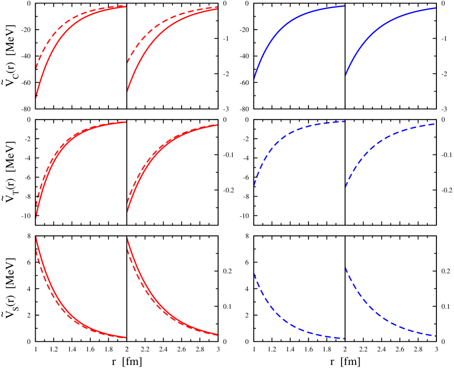
Figure 4: Isoscalar two-pion exchange potentials in coordinate space. Left (right) panels show the results with (without) explicit $\Delta$’s. Dashed and solid lines refer to the NLO and NNLO results, respectively. There are no contributions to $\tilde{V}_{C}$ ($\tilde{V}_{T,S}$) at NLO-$\Delta/\,$ (NNLO-$\Delta/\,$).

For the LECs $c_{i}$ and $b_{3}+b_{8}$, we use the values obtained in fit 1, see Tab. 1.

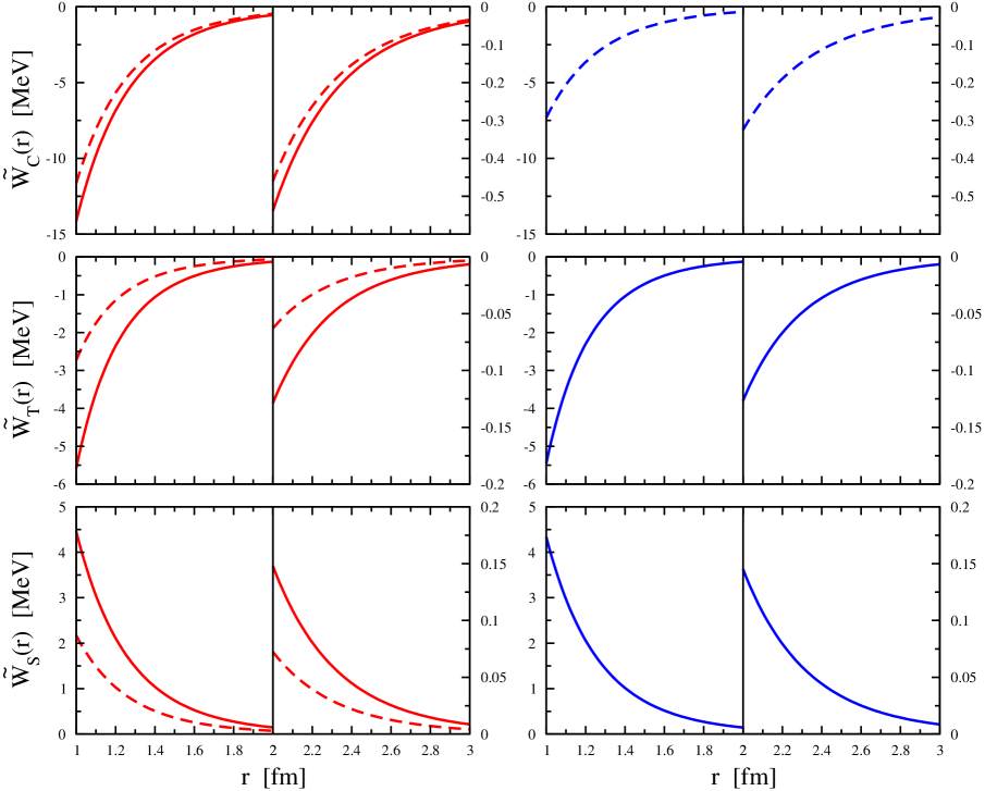
Figure 5: Isovector two-pion exchange potentials in coordinate space. Left (right) panels show the results with (without) explicit $\Delta$’s. Dashed and solid lines refer to the NLO and NNLO results, respectively. There are no contributions to $\tilde{W}_{C}$ ($\tilde{W}_{T,S}$) at NNLO-$\Delta/\,$ (NLO-$\Delta/\,$).

The results at NNLO-$\Delta/\,$ are based on the values for $c_{i}$ given in the second column of Tab. 1 (these are not very different from the ones obtained in the literature using other values of these LECs). The isoscalar central potential $\tilde{V}_{C}(r)$ is known to be the strongest part of the chiral TPEP. In EFT-$\Delta/\,$, it receives the first contribution at NNLO. The SSE leads to a much more natural convergence pattern for $\tilde{V}_{C}(r)$ with the dominant contribution being generated at NLO-$\Delta$. The correction at NNLO-$\Delta$ is still significant and produces further attraction. Notice also that the NNLO-$\Delta/\,$ result for $\tilde{V}_{C}(r)$ lies between the NLO-$\Delta$ and NNLO-$\Delta$ ones. Contrary to the central part, the isoscalar tensor and spin-spin potentials $\tilde{V}_{T,S}(r)$ as well as the isovector central potential $\tilde{W}_{C}(r)$ receive the contributions at NLO-$\Delta/\,$ with no further corrections at NNLO-$\Delta/\,$. As shown in Figs. 4 and 5, the leading contributions due to the intermediate $\Delta$-excitation turn out to be significant in all these cases while the subleading corrections (i.e. at NNLO-$\Delta$) are less important. Notice that the resulting potential $\tilde{W}_{C}(r)$ at NNLO-$\Delta$ is nearly twice as strong as at NNLO-$\Delta/\,$. The strength of the remaining isovector tensor and spin-spin parts of the potential $\tilde{W}_{T,S}(r)$ at NNLO-$\Delta/\,$ comes out remarkably close to the one obtained at the same order in the EFT without explicit $\Delta$’s, see Fig. 5. Again, contrary to EFT-$\Delta/\,$, the NLO contributions to $\tilde{W}_{T,S}(r)$ in the theory with explicit $\Delta$’s do not vanish. Let us now comment on the sensitivity of the TPEP to the value of the LEC $h_{A}$ used as an input in the determination of the LECs $c_{i}$ and $b_{3}+b_{8}$, see the discussion in section III. While the values of the LECs obtained in fits 1 and 2 for two different choices of $h_{A}$ differ significantly from each other, see Tab. 1, the resulting S- and P-wave threshold parameters nearly coincide in both cases, see Tab. 2. As demonstrated in Fig. 6, a similar trend holds also for the TPEP.

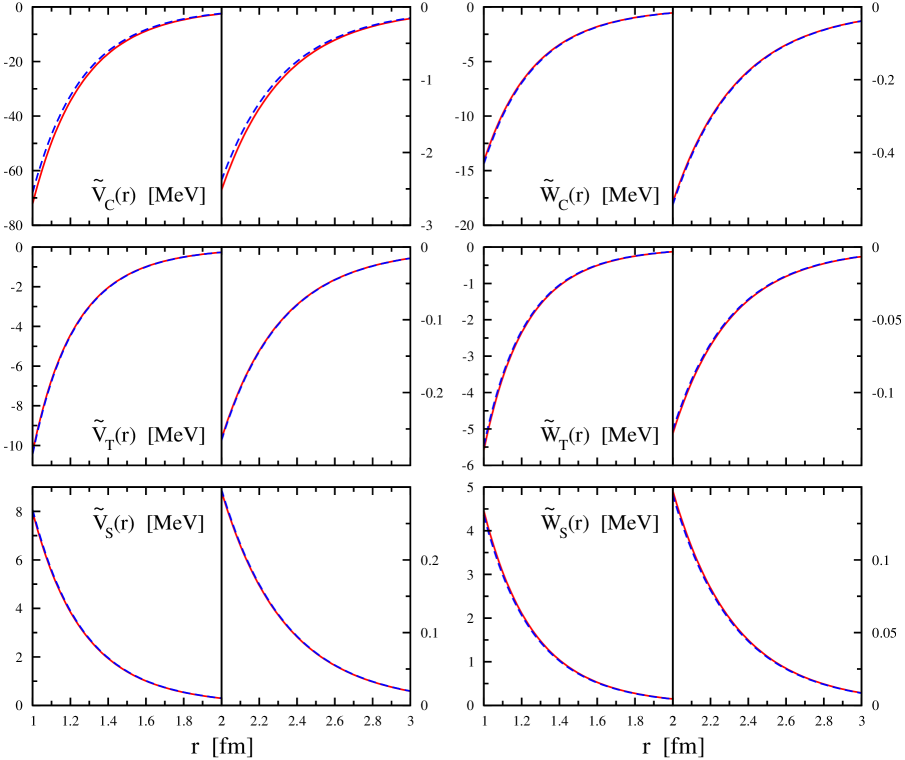
Figure 6: Sensitivity of the NNLO two-pion exchange potential to the choice of the low-energy constant $h_{A}$. Solid (dashed) lines show the NNLO potentials with $h_{A}={3}g_{A}/(2\sqrt{2})\sim 1.34$ ($h_{A}=1.05$) and the LECs $c_{i}$ chosen according to fits 1 and 2 in Tab. 1.

The only visible (but still very small) difference is observed for the isoscalar central part of the potential.

We will now consider D- and higher partial waves up to NNLO in chiral EFT with and without explicit deltas following the lines of Refs. (Kaiser:1998wa, ; Epelbaum:2003gr, ). Using Born approximation for the scattering amplitude, the phase shifts and mixing angles in the convention of Stapp et al. (Stapp:1956mz, ) are determined by the 2N potential $V$ as:

$$\delta^{sj}_{l}=-\frac{mq}{(4\pi)^{2}}\langle lsj|V|lsj\rangle\,,\quad\quad\epsilon_{j}=-\frac{mq}{(4\pi)^{2}}\langle j-1,sj|V|j+1,sj\rangle\,,$$ (4.17)

where $s$ and $j$ refer to the total spin and angular momentum, respectively, and $q$ is the nucleon CMS momentum. Clearly, such an approximation violates unitarity. This violation is small provided that the corresponding phase shifts are small. Alternatively, one can use the $K$–matrix approach in order to restore unitarity, see e.g. (Entem:2002sf, ). Here and in what follows, we adopt the same notation for the matrix elements in the $|lsj\rangle$ basis as in Ref. (Epelbaum:2004fk, ). The expressions for the partial wave decomposition can be found in appendix B of this reference.

Our results for D- F- and G-waves and for the mixing parameters $\epsilon_{2,3,4}$ are shown in Figs. 7-9.

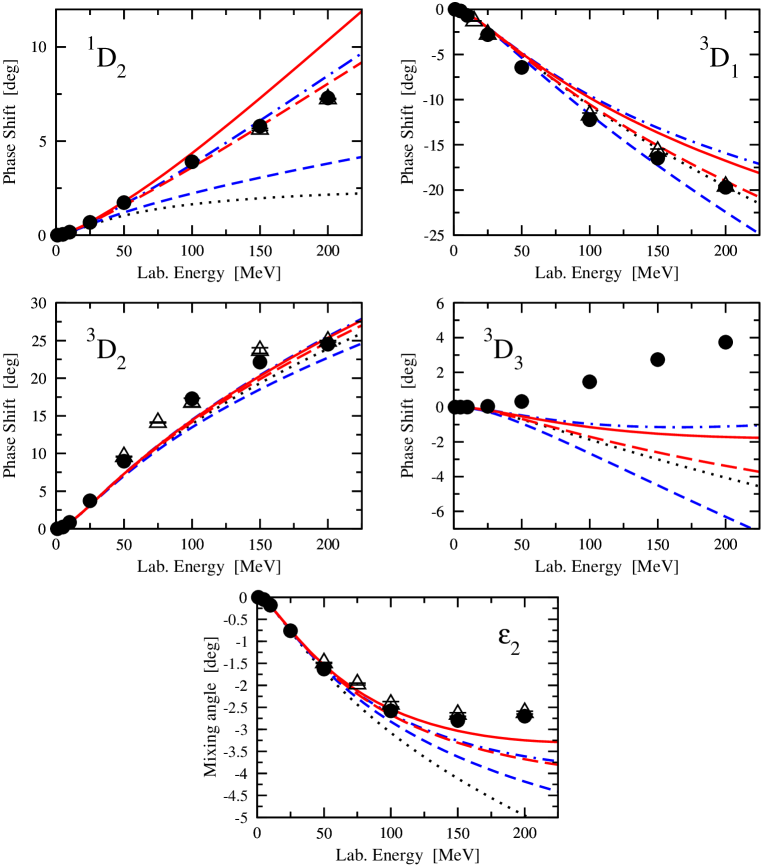
Figure 7: D–wave NN phase shifts and the mixing parameter $\epsilon_{2}$. The dotted curve is the LO prediction (i.e. based on the pure OPEP). Long-dashed (short-dashed) and solid (dashed-dotted) lines show the NLO and NNLO results with (without) the explicit $\Delta$-contributions and using the SFR with $\tilde{\Lambda}=700$ MeV. The filled circles (open triangles) depict the results from the Nijmegen multi–energy PWA (Stoks:1993tb, ; NNonline, ) (Virginia Tech single–energy PWA (SAID, )).

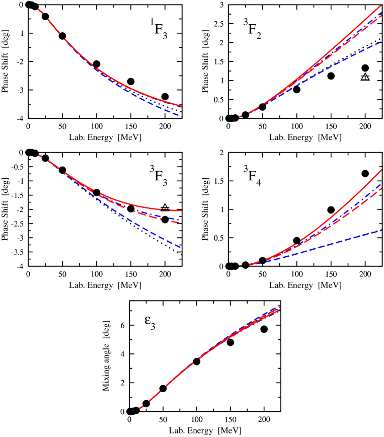
Figure 8: F–wave NN phase shifts and the mixing parameter $\epsilon_{3}$. The dotted curve is the LO prediction (i.e. based on the pure OPEP). Long-dashed (short-dashed) and solid (dashed-dotted) lines show the NLO and NNLO results with (without) the explicit $\Delta$-contributions and using the SFR with $\tilde{\Lambda}=700$ MeV. The filled circles (open triangles) depict the results from the Nijmegen multi–energy PWA (Stoks:1993tb, ; NNonline, ) (Virginia Tech single–energy PWA (SAID, )).

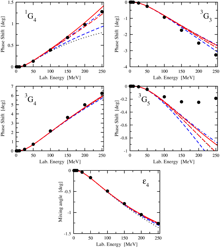
Figure 9: G–wave NN phase shifts and the mixing parameter $\epsilon_{4}$. The dotted curve is the LO prediction (i.e. based on the pure OPEP). Long-dashed (short-dashed) and solid (dashed-dotted) lines show the NLO and NNLO results with (without) the explicit $\Delta$-contributions and using the SFR with $\tilde{\Lambda}=700$ MeV. The filled circles depict the results from the Nijmegen multi–energy PWA (Stoks:1993tb, ; NNonline, ).

The two sets of the LECs obtained in fit 1 and fit 2, see Tab. 1, yield nearly the same results for all phase shifts and mixing parameters as one might expect from Fig. 6. In all channels, the convergence pattern is strongly improved in the SSE as compared to the pure chiral expansion. While the NLO corrections are small and the dominant contributions in the EFT-$\Delta/\,$ arise at NNLO, the changes between NLO and NNLO are typically much smaller than the ones between LO and NLO in the EFT-$\Delta$. The only exceptions are observed in the ${}^{3}D_{1}$, ${}^{3}D_{3}$ and ${}^{3}G_{5}$, where the NLO-$\Delta$ result appears to be close to the LO one. In all other partial waves, the results at NLO-$\Delta$ are very similar to the ones at NNLO-$\Delta/\,$. While most peripheral partial waves are reasonably well described at both NNLO-$\Delta$ and NNLO-$\Delta/\,$ using the SFR cutoff $\tilde{\Lambda}=700$ MeV, the description of the ${}^{3}D_{3}$ and ${}^{3}G_{5}$ phase shifts is rather poor. It should, however, be understood that since the phase shifts in these channels are much smaller in magnitude than in the other D- and G-waves, respectively, the observed deviations have little effect on NN scattering observables. Notice also that, especially in the ${}^{3}D_{3}$ partial wave, the contributions due to iteration of the potential in the Lippmann-Schwinger equation, which are not considered in this work, might be significant.

Finally, we would like to emphasize that the results shown in Figs. 7-9 correspond to one particular choice of the SFR cutoff $\tilde{\Lambda}=700$ MeV. The theoretical uncertainty associated with the variation of $\tilde{\Lambda}$ in the range $\tilde{\Lambda}=500\ldots 800$ MeV is exemplified in Fig.10 where the ${}^{3}F_{4}$ partial wave is shown at NNLO-$\Delta$ and NNLO-$\Delta/\,$. We note that the uncertainty at NNLO is comparable in both approaches. Note further that the results for NNLO-$\Delta/\,$ differs slightly from the one displayed in Ref. Epelbaum:2003gr due to a different choice of the LECs $c_{3,4}$.

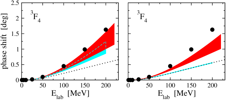
Figure 10: Theoretical uncertainty in the ${}^{3}F_{4}$ partial wave due to the variation of the SFR cutoff as described in the text. Left panel: Delta-full theory. The upper (lower) band refers to NNLO (NLO) and the dotted line is the leading order OPEP. Right panel: Same for the delta-less theory.

For a detailed discussion on the theoretical uncertainty in both peripheral and low partial waves in EFT without explicit $\Delta$’s the reader is referred to Epelbaum:2003gr ; Epelbaum:2003xx ; Epelbaum:2004fk .

V Summary and conclusions

In this paper, we have analyzed the two-nucleon two-pion-exchange potential in an effective field theory with explicit deltas (based on the so-called small scale expansion) at next-to-next-to-leading order in the chiral expansion. The pertinent results can be summarized as follows:

• At NNLO, the potential with single and double delta-excitations is shown in Figs. 1,2. It depends on 7 low-energy constants, the leading order axial-vector couplings $g_{A}$ and $h_{A}$, the dimension-two $\pi N$ LECs $c_{1},c_{2},c_{3},c_{4}$ and the combination $b_{3}+b_{8}$ from the $\pi N\Delta$ Lagrangian.

• We have determined these dimension-two LECs from a fit to the pion-nucleon S-and P-wave threshold parameters, based on the ${\cal O}(Q^{2})$ representation of the $\pi N$ scattering amplitude in the SSE, see Tables 1,2. As expected, the values for the $c_{i}$ ($i=2,3,4$) are considerably smaller than in chiral perturbation theory.

• The resulting coordinate space potentials show a more natural convergence behaviour than in the theory without deltas. In the delta-full theory, the leading contributions to the TPEP at NLO turn out to be significant while the subleading NNLO corrections are smaller, see Figs. 4,5.

• This convergence pattern is also reflected in the peripheral partial waves, that have been calculated in first Born approximation, see Figs. 7–9. Furthermore, for most partial waves the description at NLO in the delta-full theory is better than in the delta-less theory. We also find a mild improvement in some partial waves at NNLO. For the larger D-waves, these results should only be considered indicative due to the accuracy of the Born approximation.

• The theoretical uncertainty due to the variation of the SFR cutoff $\tilde{\Lambda}$ is of the expected size and comparable to the case of the delta-less theory at NNLO, see Fig. 10 for one typical case.

The work presented here paves the way to a systematic analysis of nuclear forces based on a theory with explicit deltas. A lot of work remains to be done before this will be achieved, in particular:

• The low partial waves and the deuteron require a non-perturbative treatment, i.e. the solution of the regularized Lippmann-Schwinger equation. This will be dealt with in a subsequent paper kem2 .

• To achieve a higher precision, we have to go to N³LO. To do that, one must first reconsider $\pi N$ scattering within the SSE at one-loop order, extending the work of Ref. Fettes:2000bb . It also requires a careful re-evaluation of the corresponding two- and three-pion exchange contributions with intermediate deltas. That these corrections will not be negligible follows from the calculations of sub-leading three-pion-exchanges in the delta-less theory, see Ref. Kaiser:2001dm .

• In the theory with explicit deltas, three-nucleon force (3NF) arises already at NLO. Its leading term is included in all current 3NF models and is usually referred to as the Fujita-Miyazawa force FM50 . The first corrections to it appear at NNLO, some of these are again proportional to the combination of LECs $b_{3}+b_{8}$. The ordering of various contributions to the 3NF in the theory with explicit deltas is therefore very different from the one based on the pure pion-nucleon theory, as discussed e.g. in Pandharipande:2005sx .

• Additional isospin violation effects arise in the 2NF and 3NF due to the mass splittings of the various delta charge states. These should be investigated systematically within the consistent EFT extending earlier model-dependent work Li:1998xh .

Appendix A $\pi N$ threshold coefficients at order $Q^{2}$

In this appendix we give explicit expressions for $\pi N$ threshold coefficients $a_{0+}^{\pm}$, $b_{0+}^{\pm}$ and $a_{1\pm}^{\pm}$ at order $Q^{2}$ (calculated in the SSE) used in section III to determine the corresponding LECs. These are in standard notation:

$$a_{0+}^{+} = \frac{1}{2\pi F_{\pi}^{2}(m+M_{\pi})}\,(-2c_{1}+c_{2}+c_{3})\,mM_{\pi}^{2}\,,$$

$$b_{0+}^{+} = \frac{1}{8\pi F_{\pi}^{2}m(m+M_{\pi})}\,\Big{(}2c_{1}(2m-M_{\pi})M_{\pi}+c_{2}(4m^{2}-2mM_{\pi}+M_{\pi}^{2})+c_{3}(4m^{2}-2mM_{\pi}+M_{\pi}^{2})\Big{)}\,,$$

$$a_{0+}^{-} = \frac{1}{8\pi F_{\pi}^{2}(m+M_{\pi})}\,mM_{\pi}\,,$$

$$b_{0+}^{-} = \frac{1}{32\pi F_{\pi}^{2}mM_{\pi}(m+M_{\pi})}\,(2m^{2}-2mM_{\pi}+M_{\pi}^{2})\,,$$

$$a_{1-}^{-} = -\frac{1}{24\pi F_{\pi}^{2}M_{\pi}(m+M_{\pi})}\,m\,(g_{A}^{2}-4c_{4}M_{\pi})+\frac{1}{27\pi F_{\pi}^{2}(m+M_{\pi})(M_{\pi}+\Delta)}\,m\,\Big{(}h_{A}^{2}-2h_{A}\,(b_{3}+b_{8})M_{\pi}\Big{)}\,,$$

$$a_{1-}^{+} = -\frac{1}{12\pi F_{\pi}^{2}M_{\pi}(m+M_{\pi})}\,m\,(g_{A}^{2}+2c_{3}M_{\pi})+\frac{2}{27\pi F_{\pi}^{2}(m+M_{\pi})(M_{\pi}+\Delta)}\,m\,\Big{(}h_{A}^{2}-2h_{A}\,(b_{3}+b_{8})M_{\pi}\Big{)}\,,$$

$$a_{1+}^{-} = -\frac{1}{24\pi F_{\pi}^{2}M_{\pi}(m+M_{\pi})}\,m\,(g_{A}^{2}+2c_{4}M_{\pi})$$

$${}+\frac{1}{54\pi F_{\pi}^{2}(m+M_{\pi})(M_{\pi}^{2}-\Delta^{2})}\,m\,\Big{(}h_{A}^{2}(2M_{\pi}+\Delta)+2h_{A}\,(b_{3}+b_{8})M_{\pi}(M_{\pi}+2\Delta)\Big{)}\,,$$

$$a_{1+}^{+} = \frac{1}{24\pi F_{\pi}^{2}M_{\pi}(m+M_{\pi})}\,m\,(g_{A}^{2}-4c_{3}M_{\pi})$$ (A.1)

$${}-\frac{1}{27\pi F_{\pi}^{2}(m+M_{\pi})(M_{\pi}^{2}-\Delta^{2})}\,m\,\Big{(}h_{A}^{2}(M_{\pi}+2\Delta)+2h_{A}\,(b_{3}+b_{8})M_{\pi}(2M_{\pi}+\Delta)\Big{)}\,.$$

References

- (1) P. F. Bedaque and U. van Kolck, Ann. Rev. Nucl. Part. Sci. 52, 339 (2002), nucl-th/0203055.
- (2) E. Epelbaum, Prog. Part. Nucl. Phys. 57, 654 (2006), nucl-th/0509032.
- (3) N. Fettes and U.-G. Meißner, Nucl. Phys. A 676, 311 (2000), hep-ph/0002162.
- (4) T. R. Hemmert, B. R. Holstein, and J. Kambor, J. Phys. G 24, 1831 (1998), hep-ph/9712496.
- (5) N. Fettes and U.-G. Meißner, Nucl. Phys. A 679, 629 (2001), hep-ph/0006299.
- (6) C. Hanhart, Phys. Rept. 397, 155 (2004), hep-ph/0311341.
- (7) C. Ordóñez, L. Ray, and U. van Kolck, Phys. Rev. C 53, 2086 (1996), hep-ph/9511380.
- (8) N. Kaiser, S. Gerstendorfer, and W. Weise, Nucl. Phys. A 637, 395 (1998), nucl-th/9802071.
- (9) E. Epelbaum, W. Glöckle, and U.-G. Meißner, Eur. Phys. J. A 19, 125 (2004), nucl-th/0304037.
- (10) V. Bernard, N. Kaiser, and U.-G. Meißner, Nucl. Phys. A 615, 483 (1997), hep-ph/9611253.
- (11) N. Fettes, U.-G. Meißner, and S. Steininger, Nucl. Phys. A 640, 199 (1998), hep-ph/9803266.
- (12) N. Kaiser, R. Brockmann, and W. Weise, Nucl. Phys. A 625, 758 (1997), nucl-th/9706045.
- (13) E. Epelbaum, W. Glöckle, and U.-G. Meißner, Nucl. Phys. A 747, 362 (2005), nucl-th/0405048.
- (14) E. Epelbaum, W. Glöckle, and U.-G. Meißner, Eur. Phys. J. A 19, 401 (2004), nucl-th/0308010.
- (15) H. P. Stapp, T. J. Ypsilantis, and N. Metropolis, Phys. Rev. 105, 302 (1957).
- (16) D. R. Entem and R. Machleidt, Phys. Rev. C66, 014002 (2002), nucl-th/0202039.
- (17) V. G. J. Stoks, R. A. M. Klomp, M. C. M. Rentmeester, and J. J. de Swart, Phys. Rev. C 48, 792 (1993).
- (18) NN-Online program, M. C. M. Rentmeester et al., http://nn-online.org.
- (19) SAID on-line program, R. A.Arndt et al., http://gwdac.phys.gwu.edu.
- (20) H. Krebs, E. Epelbaum and U.-G. Meißner, in preparation.
- (21) N. Kaiser, Phys. Rev. C 63, 044010 (2001), nucl-th/0101052.
- (22) J.-I. Fujita and H. Miyazawa, Prog. Theor. Phys. 17, 360 (1957)
- (23) V. R. Pandharipande, D. R. Phillips and U. van Kolck, Phys. Rev. C 71, 064002 (2005), nucl-th/0501061.
- (24) G. Q. Li and R. Machleidt, Phys. Rev. C 58, 3153 (1998), nucl-th/9807080.