TUM-T39-07-04

Chiral Perturbation Theory and the first moments of the Generalized Parton Distributions in a Nucleon

Marina Dorati^a,b, Tobias A. Gail^b and Thomas R. Hemmert^b

^a Dipartimento di Fisica Nucleare e Teorica
Universita’ degli Studi di Pavia and INFN, Pavia, Italy
^b Physik-Department, Theoretische Physik T39
TU München, D-85747 Garching, Germany

We discuss the first moments of the parity-even Generalized Parton Distributions (GPDs) in a nucleon, corresponding to six (generalized) vector form factors. We evaluate these fundamental properties of baryon structure at low energies, utilizing the methods of covariant Chiral Perturbation Theory in the baryon sector (BChPT). Our analysis is performed at leading-one-loop order in BChPT, predicting both the momentum and the quark-mass dependence for the three (generalized) isovector and (generalized) isoscalar form factors, which are currently under investigation in lattice QCD analyses of baryon structure. We also study the limit of vanishing four-momentum transfer where the GPD-moments reduce to the well known moments of Parton Distribution Functions (PDFs). For the isovector moment $\langle x\rangle_{u-d}$ our BChPT calculation predicts a new mechanism for chiral curvature, connecting the high values for this moment typically found in lattice QCD studies for large quark masses with the smaller value known from phenomenology. Likewise, we analyze the quark-mass dependence of the isoscalar moments in the forward limit and extract the contribution of quarks to the total spin of the nucleon. We close with a first glance at the momentum dependence of the isoscalar C-form factor of the nucleon.

1 Introduction

Understanding the structure of the nucleon arising from the underlying dynamics of quarks and gluons—governed by the theory of Quantum-Chromo-Dynamics (QCD)—is still one of the major challenges in nuclear physics. About a decade ago the concept of Generalized Parton Distributions (GPDs) has emerged among theorists, constituting a universal framework bringing a host of seemingly disparate nucleon structure observables like form factors, moments of parton distribution functions, etc. under one theoretical roof. For reviews of this very active field of research we refer to [1].

Working in twist-2 approximation, the parity-even part of the structure of the nucleon is encoded via two Generalized Parton Distribution functions $\textit{H}^{q}(x,\xi,t)$ and $\textit{E}^{q}(x,\xi,t)$. For a process where the incoming (outgoing) nucleon carries the four-momentum $p_{1}^{\mu}\,(p_{2}^{\mu})$ we define two new momentum variables

$$\Delta^{\mu}=p_{2}^{\mu}-p_{1}^{\mu};\quad\bar{p}=(p_{1}^{\mu}+p_{2}^{\mu})/2.$$ (1)

The GPD variable $x$ then corresponds to Bjorken-$x$, which in the parton model of the nucleon can be interpreted as the fraction of the total momentum of the nucleon carried by the probed quark $q$. $t\equiv\Delta^{2}$ denotes the total four-momentum transfer (squared) to the nucleon, whereas the “skewdness” variable $\xi=-n\cdot\Delta/2$ with $n\cdot\bar{p}=1$ interpolates between the $t$- and the $x$-dependence of the GPDs. Throughout this work we focus on the non-perturbative regime of QCD: $-t<<1$ GeV², i.e. the realm of strongly interacting matter in our solar system making up humans, planets, etc.. We are therefore utilizing the methods of Chiral Effective Field Theory (ChEFT) for our analysis [2].

The 3-dimensional parameter space of GPDs is vast and rich in information about nucleon structure. The experimental program of their determination is only at the beginning at laboratories like CERN, Desy, JLAB, …[1]. However, moments of GPDs can be interpreted much easier and are connected to well-established hadron structure observables. E.g. the zero-th order (Mellin-) moments in the variable $x$ correspond to the contribution of quark $q$ to the well known Dirac and Pauli form factors $F_{1}(t),\,F_{2}(t)$ of the nucleon:

$$\int_{-1}^{1}dx\,x^{0}\,\textit{H}^{q}(x,\xi,t) = F_{1}^{q}(t),$$ (2)

$$\int_{-1}^{1}dx\,x^{0}\,\textit{E}^{q}(x,\xi,t) = F_{2}^{q}(t).$$ (3)

For the case of 2 light flavors the isoscalar and isovector Dirac and Pauli form factors of the nucleon have been studied at low values of $t$ at the one-loop level in Chiral Effective Field Theory, both in non-relativistic [3] and in covariant [4, 5] schemes. The chiral extrapolation of these form factors for lattice QCD data with the help of ChEFT has been discussed in refs.[8, 9, 10, 11], whereas the status of the experimental situation is reviewed in ref.[12].

In this work we want to focus on the first moments in $x$ of these nucleon GPDs

$$\int_{-1}^{1}dx\,x\,\textit{H}^{q}(x,\xi,t) = A_{2,0}^{q}(t)+(-2\xi)^{2}\textit{C}_{2,0}^{q}(t),$$ (4)

$$\int_{-1}^{1}dx\,x\,\textit{E}^{q}(x,\xi,t) = B_{2,0}^{q}(t)-(-2\xi)^{2}\textit{C}_{2,0}^{q}(t),$$ (5)

where one encounters three generalized form factors $A_{2,0}^{q}(t),\,B_{2,0}^{q}(t),\,C_{2,0}^{q}(t)$ of the nucleon for each quark flavor $q$. For the case of 2 light flavours the generalized isoscalar and isovector form factors have been analyzed in a series of papers at leading-one-loop order in the non-relativistic framework of HBChPT, starting with the pioneering analyses of Chen and Ji as well as Belitsky and Ji [13, 14, 15, 16]. In this work we want to provide the first analysis of these generalized form factors utilizing the methods of covariant Baryon Chiral Perturbation Theory (BChPT) for 2 light flavors, pioneered in ref.[4]. Utilizing a variant of Infrared Regularization [17] for the loop diagrams, our BChPT formalism is constructed in such a way that we exactly reproduce the corresponding HBChPT result of the same chiral order in the limit of small pion masses.

We note that (at $t=0$) a covariant BChPT calculation differs from a non-relativistic one—provided both are performed at the same chiral order $D$—by an infinite series of terms $\sim(m_{\pi}/M_{0})^{n}$, where $M_{0}$ denotes the mass of the nucleon (in the chiral limit), estimated to be around 890 MeV [19]. Such terms quickly become relevant once the pion mass $m_{\pi}$ takes on values larger than 140 MeV, as it typically occurs in present-day lattice QCD simulations of (generalized) form factors. Aside from this resummation property in $(1/M_{0})^{n}$, we note that the power-counting analysis determining possible operators and allowed topologies for loop diagrams at a particular chiral order (see section 3.3) is identical between covariant and non-relativistic frameworks. Both schemes organize a perturbative calculation as a power series in $(p/\Lambda_{\chi})^{D}$, where $p$ corresponds either to a small 3-momentum or to the mass of the pion, whereas $\Lambda_{\chi}\approx 1.2$ GeV denotes the scale of chiral symmetry breaking. Finally, we would like to note that the first moments of nucleon GPDs have also been studied in constituent quark models (e.g. see ref.[20]) and chiral quark soliton models (e.g. see ref.[21]) of the nucleon, which—in contrast to ChEFT—can also provide dynamical insights into the short-distance structure present in the generalized form factors.

This paper is organized as follows: In the next section we specify the operators with which we are going to obtain information on the three generalized isoscalar and the three generalized isovector form factors of the nucleon. In section 3 we portray the effective chiral Lagrangean required for the calculation, immediately followed by the sections containing our leading-one-loop results of the generalized form factors in the isovector (section 4) and in the isoscalar (section 5) matrix elements. A summary of the main results concludes this paper, while a few technical details regarding the calculation of the amplitudes in covariant BChPT are relegated to the appendices.

2 Extracting the First Moments of GPDs

2.1 Generalized Form Factors of the Nucleon

In Eqs.(4,5) of the Introduction it was shown that the first moments of nucleon GPDs are connected to three generalized form factors. In lattice QCD one can directly access the contribution of quark flavor $q$ to these generalized form factors of the nucleon by evaluating the matrix element [1]

$$i\langle p^{\prime}|\overline{q}\gamma_{\{\mu}\overleftrightarrow{\textit{D}}_{\nu\}}\,q|p\rangle = \overline{u}(p^{\prime})\bigg{[}{\textit{A}_{2,0}^{q}(\Delta^{2})}\gamma_{\{\mu}\overline{p}_{\nu\}}-\frac{{\textit{B}_{2,0}^{q}(\Delta^{2})}}{2M_{N}}\>\Delta^{\alpha}i\sigma_{\alpha\{\mu}\overline{p}_{\nu\}}+\frac{{\textit{C}_{2,0}^{q}(\Delta^{2})}}{M_{N}}\>\Delta_{\{\mu}\Delta_{\nu\}}\bigg{]}\,u(p).$$ (6)

The brackets $\{\ldots\}$ denote the completely symmetrized and traceless combination of all indices in an operator. $u\,(\overline{u})$ is a Dirac spinor of the incoming (outgoing) nucleon of mass $M_{N}$, for which the quark matrix-element is evaluated. In ChEFT we employ the same philosophy and also extract information about the first moments of nucleon GPDs of Eq.(4,5) via a calculation of the generalized form factors according to Eq.(6).

Studying a strongly interacting system with 2 light flavors in the non-perturbative regime of QCD, with the methods of ChEFT one can only directly access the singlet $(s)$ and triplet $(v)$ contributions of the quarks to the the three form factors:

$$i\langle p^{\prime}|\overline{q}\gamma_{\{\mu}\overleftrightarrow{\textit{D}}_{\nu\}}\,q|p\rangle_{u+d} = \overline{u}(p^{\prime})\bigg{[}{\textit{A}_{2,0}^{s}(\Delta^{2})}\gamma_{\{\mu}\overline{p}_{\nu\}}-\frac{{\textit{B}_{2,0}^{s}(\Delta^{2})}}{2M_{N}}\>\Delta^{\alpha}i\sigma_{\alpha\{\mu}\overline{p}_{\nu\}}+\frac{{\textit{C}_{2,0}^{s}(\Delta^{2})}}{M_{N}}\>\Delta_{\{\mu}\Delta_{\nu\}}\bigg{]}\,\frac{{\bf 1}}{2}\,u(p),$$

$$i\langle p^{\prime}|\overline{q}\gamma_{\{\mu}\overleftrightarrow{\textit{D}}_{\nu\}}\,q|p\rangle_{u-d} = \overline{u}(p^{\prime})\bigg{[}{\textit{A}_{2,0}^{v}(\Delta^{2})}\gamma_{\{\mu}\overline{p}_{\nu\}}-\frac{{\textit{B}_{2,0}^{v}(\Delta^{2})}}{2M_{N}}\>\Delta^{\alpha}i\sigma_{\alpha\{\mu}\overline{p}_{\nu\}}+\frac{{\textit{C}_{2,0}^{v}(\Delta^{2})}}{M_{N}}\>\Delta_{\{\mu}\Delta_{\nu\}}\bigg{]}\,\frac{\tau^{a}}{2}\,u(p).$$

Note that the shown 2 x 2 unit matrix ${\bf 1}$ and the Pauli-matrices $\tau^{a},\,a=1,2,3$ on the right hand sides of Eqs.(LABEL:defs,LABEL:defv) operate in the space of a (proton,neutron) doublet field.

At present, not much is known yet experimentally about the momentum dependence of these 6 form factors. The main source of information at the moment is provided by lattice QCD studies of these objects (e.g. see refs.[22, 23, 24]). Given that present-day lattice simulations work with quark-masses much larger than those realized for $u$ and $d$ quarks in the standard model, one also needs to know the quark-mass dependence of all 6 form factors, in order to extrapolate the lattice QCD results down to the real world of light $u$ and $d$ quarks. This information is also encoded in the ChEFT results, typically expressed in form of a pion-mass dependence of the observables under study. (The connection between the explicit breaking of chiral symmetry due to non-zero quark-masses and the resulting effective pion-mass is addressed in section 3.2.)

The need for a chiral extrapolation of lattice QCD results for the generalized form factors of the nucleon leads to a further complication in the analysis: One needs to be aware that it is common practice in current lattice QCD analyses that the mass parameter $M_{N}$ in Eqs.(LABEL:defs,LABEL:defv) does not correspond to the physical mass of a nucleon, instead, it represents a (larger) nucleon mass consistent with the values of the quark-masses employed in the simulation. Fortunately the quark-mass dependence of $M_{N}$ has been studied in detail in ChEFT, both in non-relativistic [6] and in covariant frameworks [19]. The next-to-leading one-loop chiral formulae of ref.[19] provide a stable extrapolation function up to effective pion-masses $\sim 600$ MeV. In this work we utilize the ${\cal O}(p^{4})$ BChPT result (see Appendix C)

$$M_{N}(m_{\pi}) = M_{0}-4c_{1}m_{\pi}^{2}+\frac{3g_{A}^{2}m_{\pi}^{3}}{32\pi^{2}F_{\pi}^{2}\sqrt{4-\frac{m_{\pi}^{2}}{M_{0}^{2}}}}\left(-4+\frac{m_{\pi}^{2}}{M_{0}^{2}}+4c_{1}\frac{m_{\pi}^{4}}{M_{0}^{3}}\right)\arccos{\left(\frac{m_{\pi}}{2M_{0}}\right)}$$ (9)

$$+4e_{1}^{r}(\lambda)m_{\pi}^{4}-\frac{3m_{\pi}^{4}}{128\pi^{2}F_{\pi}^{2}}\Bigg{[}\left(\frac{6g_{A}^{2}}{M_{0}}-c_{2}\right)+4\left(\frac{g_{A}^{2}}{M_{0}}-8c_{1}+c_{2}+4c_{3}\right)\log{\left(\frac{m_{\pi}}{\lambda}\right)}\Bigg{]}$$

$$-\frac{3c_{1}g_{A}^{2}m_{\pi}^{6}}{8\pi^{2}F_{\pi}^{2}M_{0}^{2}}\log{\left(\frac{m_{\pi}}{M_{0}}\right)}+{\cal O}(p^{5}).$$

in order to correct for the mass effects in Eqs.(LABEL:defs,LABEL:defv). The coupling constants occurring in this formula are described in detail in ref.[19]. Possible effects of higher orders can be estimated as ${\cal O}(p^{5})\sim\delta_{M}\frac{m_{\pi}^{5}}{\Lambda_{\chi}^{4}}$, where $\delta_{M}$ could be varied within natural size estimates $-3,\ldots,+3$ [18].

We note that the trivial, purely kinematical effect of $M_{N}=M_{N}(m_{\pi})$ in Eqs.(LABEL:defs,LABEL:defv) could induce quite a strong quark-mass dependence into the form factors $B_{2,0}^{s,v}(t),\,C_{2,0}^{s,v}(t)$ and might even be able to mask any “intrinsic” quark-mass dependence in these form factors. We are reminded of the analysis of the Pauli form factors $F_{2}^{s,v}(t)$ in ref.[9], where the absorption of the analogous effect into a “normalized magneton” even led to a different slope (!) for the isovector anomalous magnetic moment $\kappa_{v}=F_{2}^{v}(t=0)$ when compared to the quark mass dependence of the “not-normalized” lattice data. We therefore urge the readers that this effect should be taken into account in any quantitative (future) analysis of the quark-mass dependence of the generalized form factors $B_{2,0}^{s,v}(t),\,C_{2,0}^{s,v}(t)$ as well. For completeness—based on the extensive studies of ref.[19]—we suggest a set of couplings in table 1 to be used in Eq.(9) from which one can estimate the impact of this effect in the matrix elements of Eqs.(LABEL:defs, LABEL:defv).

$g_{A}$	$F_{\pi}$ [GeV]	$M_{0}$ [GeV]	$c_{1}$ [GeV-1]	$c_{2}$ [GeV-1]	$c_{3}$ [GeV-1]	$e_{1}^{r}$(1GeV) [GeV-3]	$\delta_{M}$
1.2	0.0924	0.889	-0.817	3.2	-3.4	1.44	0

Table 1: Input values used in this work for the numerical analysis of the chiral extrapolation functions.

Finally, we note that in the forward limit $t\rightarrow 0$ the generalized form factors $A_{2,0}^{s,v}(t=0)$ can be understood as moments of the ordinary Parton Distribution Functions (PDFs) $q(x),\,\bar{q}(x)$ [1]:

$$\langle x\rangle_{u\pm d} = A_{2,0}^{s,v}(t=0)=\int_{0}^{1}dx\,x\left(q(x)+\bar{q}(x)\right)_{u\pm d}.$$ (10)

Experimental results exist for $\langle x\rangle$ in proton- and “neutron-” targets, from which one can estimate the isoscalar and isovector quark contributions at the physical point [26] at a regularization scale $\mu$. In this work we choose $\mu=2$ GeV for our comparisons with phenomenology. In section 4.1 we attempt to connect the physical value for $\langle x\rangle_{u-d}$ with recent (preliminary) lattice QCD results from the LHPC collaboration [24], whereas in section 5.1 we analyse the quark-mass dependence of $\langle x\rangle_{u+d}$ with (quenched) lattice QCD results from the QCDSF collaboration [22].

2.2 Generalized Form Factors of the Pion

The first moment of a generalized parton distribution function in a pion $\textit{H}^{q}_{\pi}(x,\xi,t)$ can be defined analogously to the case of a nucleon discussed above. One obtains [1]

$$\int_{-1}^{1}dx\,x\,\textit{H}^{q}_{\pi}(x,\xi,t) = A_{\pi}^{q}(t)+(-2\xi)^{2}\textit{C}_{\pi}^{q}(t).$$ (11)

The two functions $A_{\pi}^{q}(t),\,C_{\pi}^{q}(t)$ are the generalized form factors of the pion, generated by contributions of quark flavor $q$. In the forward limit one recovers the first moment of the ordinary parton distribution functions in a pion:

$$\langle x\rangle_{\pi} = A_{\pi}^{q}(t=0)=\int_{0}^{1}dx\,x\left(q(x)+\bar{q}(x)\right).$$ (12)

In the analysis of the isoscalar GPD moments of a nucleon we encounter tensor fields directly interacting with the pion cloud of the nucleon. One therefore needs to understand the relevant pion-tensor couplings in terms of the 2 generalized form factors $A_{\pi}(t),\,C_{\pi}(t)$. We note that the two generalized form factors of the pion have been analysed at one-loop level already in ref.[27] for the total sum of quark and gluon contributions, whereas the quark contribution to the form factors as defined in Eq.(11) has been the focus of the more recent work [28].

3 Formalism

3.1 Leading Order Nucleon Lagrangean

The well-known leading order Lagrangean in BChPT is given as [4]

$$\mathcal{L}_{\pi N}^{(1)}=\overline{\psi}_{N}\left\{i\gamma^{\mu}D_{\mu}-M_{0}+\frac{g_{A}^{0}}{2}\gamma^{\mu}\gamma_{5}u_{\mu}\right\}\psi_{N},$$ (13)

with

$$D_{\mu}\psi_{N} = \left\{\partial_{\mu}-iv_{\mu}^{(0)}+\frac{1}{2}\left[u^{\dagger},\partial_{\mu}u\right]-\frac{i}{2}u^{\dagger}\left(\tilde{v}_{\mu}+\tilde{a}_{\mu}\right)u-\frac{i}{2}u\left(\tilde{v}_{\mu}-\tilde{a}_{\mu}\right)u^{\dagger}\right\}\psi_{N},$$ (14)

$$u_{\mu} = iu^{\dagger}\nabla_{\mu}Uu^{\dagger}.$$ (15)

$U\equiv u^{2}$ corresponds to a non-linear realization of the (quasi-) Goldstone boson fields, $\tilde{v}_{\mu},\,\tilde{a}_{\mu}$ denote arbitrary isovector vector, axial-vector background fields, while $v_{\mu}^{(0)}$ is the isosinglet vector background field. The covariant derivative $\nabla_{\mu}U$ is defined as

$$\nabla_{\mu}U=\partial_{\mu}U-i\left(\tilde{v}_{\mu}+\tilde{a}_{\mu}\right)U+iU\left(\tilde{v}_{\mu}-\tilde{a}_{\mu}\right).$$ (16)

Finally, we note that the coupling $g_{A}^{0}$ denotes the axial-coupling of the nucleon (in the chiral limit), whereas $M_{0}$ corresponds to the nucleon mass (in the chiral limit).

We now want to extend this Lagrangean to the interaction between external tensor fields and a strongly interacting system at low energies. In this work we focus on symmetric, traceless tensor fields with positive parity in order to calculate the generalized form factors of the nucleon. In particular, we utilize the (chiral) tensor structures

$$V_{\mu\nu}^{\pm} = \frac{1}{2}\left(g_{\mu\alpha}g_{\nu\beta}+g_{\mu\beta}g_{\nu\alpha}-\frac{2}{d}g_{\mu\nu}g_{\alpha\beta}\right)\times\left(u^{\dagger}V^{\alpha\beta}_{R}u\pm uV^{\alpha\beta}_{L}u^{\dagger}\right),$$

$$V_{\mu\nu}^{0} = \frac{1}{2}\left(g_{\mu\alpha}g_{\nu\beta}+g_{\mu\beta}g_{\nu\alpha}-\frac{2}{d}g_{\mu\nu}g_{\alpha\beta}\right)\tilde{v}^{\alpha\beta}\;\frac{{\bf 1}}{2}\;.$$ (17)

We note, that the chiral tensor fields $V_{\mu\nu}^{\pm}$ transform as $hV_{\mu\nu}^{\pm}h^{\dagger}$ under chiral rotations, where $h$ corresponds to the standard compensator field of 2 flavour ChPT [4], whereas $V_{\mu\nu}^{0}$ is a chiral singlet. Chiral transformation properties for all remaining structures in our Lagrangeans are standard and can be found in the literature. The right- and left-handed fields $V_{\alpha\beta}^{(R,L)}$ are related to the symmetric (isovector) tensor fields of definite parity $v_{\alpha\beta}^{i},\,a_{\alpha\beta}^{i},\,i=1,2,3$ via

$$V_{\alpha\beta}^{R} = \left(v_{\alpha\beta}^{i}+a_{\alpha\beta}^{i}\right)\times\frac{\tau^{i}}{2}\,,$$

$$V_{\alpha\beta}^{L} = \left(v_{\alpha\beta}^{i}-a_{\alpha\beta}^{i}\right)\times\frac{\tau^{i}}{2}\,,$$ (18)

while $\tilde{v}_{\alpha\beta}$ denotes the symmetric isoscalar tensor field of positive parity.

In order to study possible interactions with external tensor fields originating from the leading order Lagrangean Eq.(13), we re-write it into the equivalent form

$$\mathcal{L}_{t\pi N}^{(0,1)} = \overline{\psi}_{N}\left\{\frac{1}{2}\left(i\gamma^{\mu}\widetilde{g_{\mu\nu}}\overrightarrow{D}^{\nu}-i\overleftarrow{D}^{\nu}\widetilde{g_{\mu\nu}}\gamma^{\mu}\right)-M_{0}+\ldots\right\}\psi_{N},$$ (19)

with

$$\widetilde{g_{\mu\nu}} = g_{\mu\nu}+a_{2,0}^{s}V_{\mu\nu}^{0}+\frac{a_{2,0}^{v}}{2}V_{\mu\nu}^{+}.$$ (20)

The coupling $a_{2,0}^{s}\,(a_{2,0}^{v})$ has been defined such that it corresponds to the chiral limit value of $\langle x\rangle_{u-d}$ $(\langle x\rangle_{u+d})$ defined in Eq.(10). We note that the coupling $a_{2,0}^{s}$ is allowed to be different from unity, as we only sum over the $u+d$ quark contributions in the isoscalar moments, but neglect the contributions from gluons. While this separation between quark- and gluon-contributions does not occur in nature, it can be implemented in lattice QCD analyses at a fixed renormalization scale (e.g see refs.[22, 23, 24]).

While the construction of the parity-even tensor interactions with a strongly interacting system started from the ${\cal O}(p)$ BChPT Lagrangean, inspection of the resulting Lagrangean Eq.(19) reveals that the leading interactions actually start out at ${\cal O}(p^{0})$, as we do not assign a chiral power $p^{n}$ to any of the tensor fields. Furthermore, symmetries allow the addition of the parity-odd tensor interaction $\sim V_{\mu\nu}^{-}$. We finally obtain

$$\mathcal{L}_{t\pi N}^{(0)} = \frac{1}{2}\overline{\psi}_{N}\left\{i\gamma^{\mu}\left(a_{2,0}^{s}V_{\mu\nu}^{0}+\frac{a_{2,0}^{v}}{2}V_{\mu\nu}^{+}+\frac{\Delta a_{2,0}^{v}}{2}V_{\mu\nu}^{-}\gamma_{5}\right)\overrightarrow{D}^{\nu}\right.$$ (21)

$$\left.\quad\quad-i\overleftarrow{D}^{\nu}\gamma^{\mu}\left(a_{2,0}^{s}V_{\mu\nu}^{0}+\frac{a_{2,0}^{v}}{2}V_{\mu\nu}^{+}+\frac{\Delta a_{2,0}^{v}}{2}V_{\mu\nu}^{-}\gamma_{5}\right)\right\}\psi_{N},$$

with the coupling $\Delta a_{2,0}^{v}$ corresponding to the chiral limit value of the axial quantity $\langle\Delta x\rangle_{u-d}$ [29].

The ${\cal O}(p^{1})$ part of the leading order pion-nucleon Lagrangean in the presence of external symmetric, traceless tensor fields with positive parity then reads

$$\mathcal{L}_{t\pi N}^{(1)} = \overline{\psi}_{N}\left\{i\gamma^{\mu}D_{\mu}-M_{0}+\frac{g_{A}^{0}}{2}\gamma^{\mu}\gamma_{5}u_{\mu}+\frac{b_{2,0}^{v}}{8M_{0}}\bigg{(}i\sigma_{\alpha\mu}\>\left[\overrightarrow{D}^{\alpha},V^{\mu\nu}_{+}\right]\overrightarrow{D}_{\nu}+h.c.\bigg{)}\right.$$ (22)

$$\left.\quad\quad+\frac{b_{2,0}^{s}}{4M_{0}}\bigg{(}i\sigma_{\alpha\mu}\>\left[\overrightarrow{\nabla}^{\alpha},V^{\mu\nu}_{0}\right]\overrightarrow{D}_{\nu}+h.c.\bigg{)}+\ldots\right\}\psi_{N},$$

where we have introduced $\nabla^{\alpha}=\partial^{\alpha}-iv_{(0)}^{\alpha}$. The two new couplings $b_{2,0}^{v},\,b_{2,0}^{s}$ can be interpreted as the chiral limit values of the form factors $B_{2,0}^{v}(0),\;B_{2,0}^{s}(0)$ in the limit $t\rightarrow 0$. No further structures enter our calculation at this order. Finally, we note that the coupling $b_{2,0}^{s}$ is only allowed to exist because we do not sum over the gluon contributions in the isoscalar moments, otherwise this form factor is bound to vanish in the forward limit $B_{2,0}^{q+g}(t=0)\equiv 0$ [30].

3.2 Consequences for the Meson Lagrangean

The choice of assigning the chiral power $p^{0}$ to the symmetric tensor fields $V_{\mu\nu}^{L,R,0}$ also has the consequence that the well-known leading-order chiral Lagrangean for 2 light flavours in the meson sector [31] is modified:

$$\mathcal{L}_{t\pi\pi}^{(2)}=\frac{F_{0}^{2}}{4}\;Tr\left[\nabla_{\mu}U^{\dagger}\left(g^{\mu\nu}+4x_{\pi}^{0}V^{\mu\nu}_{0}\right)\nabla_{\nu}U+\chi^{\dagger}U+\chi U^{\dagger}\right].$$ (23)

We note that the new coupling $x_{\pi}^{0}$ has been defined such that it corresponds to the chiral limit value of $\langle x\rangle_{\pi}$ of Eq.(12). It is allowed to differ from unity because we only sum over the quark-distribution functions in the isoscalar channel and neglect the contributions from gluons.

The explicit breaking of chiral symmetry via the finite quark masses is encoded via

$$\chi=2\,B_{0}\left(\tilde{s}+i\tilde{p}\right),$$ (24)

if one switches off the external pseudoscalar background field $\tilde{p}$ and assigns the 2-flavour quark mass-matrix ${\it M_{q}}$ to the scalar background field $\tilde{s}$. To the order we are working here we obtain the resulting pion mass $m_{\pi}$ via

$$m_{\pi}^{2}=2\,B_{0}\,\hat{m}+{\cal O}({\it M_{q}}^{2}),$$ (25)

where $\hat{m}=(m_{u}+m_{d})/2$ and $B_{0}$ corresponds to the value of the chiral condensate. The other free parameter at this order $F_{0}$ can be identified with the value of the pion-decay constant (in the chiral limit).

3.3 Power-counting with tensor fields in BChPT

We start from the general power-counting formula of Baryon ChPT:

$$D = 2L+1+\sum_{d}(d-2)N_{d}^{M}+\sum_{d}(d-1)N_{d}^{MB}.$$ (26)

$D$ denotes the chiral dimension $p^{D}$ of a particular Feynman Diagram, $L$ counts the number of loops in the diagram, whereas the variables $N_{d}^{M,\,MB}$ count the number of vertices of chiral dimension $d$ from the pion $(M)$ and pion-Nucleon $(MB)$ Lagrangeans.

To leading order we only have the tree level contributions from the $p^{0}$-Lagrangean of Eq.(21) with $L=0,\,N_{2}^{M}=0,\,N_{0}^{MB}=1$, resulting in $D=0$.

At next-to-leading order $D=1$ we find additional tree level contributions from the $p^{1}$ Lagrangean of Eq.(22) with $L=0,\,N_{2}^{M}=0,\,N_{1}^{MB}=1$.

The first loop contributions enter at $D=2$ with $L=1,\,N_{2}^{M}=0,\,N_{0}^{MB}=1$ plus possible contributions from $N_{1}^{MB}$. The corresponding diagrams are shown in Fig.1. Diagram (e) in that Figure represents (loop) corrections from the nucleon Z-factor (given in appendix C) which at this order renormalize only the tree-level tensor couplings of the $p^{0}$-Lagrangean. Note that there is an additional possibility of obtaining $D=2$ contributions via $L=0,\,N_{2}^{M}=0,\,N_{2}^{MB}=1$, corresponding to further tree level contributions discussed in the next subsection.

In this first paper we will stop with our analysis of the generalized form factors at the $D=2$, i.e. ${\cal O}(p^{2})$ level, corresponding to a (covariant) leading-one-loop calculation. The next-to-leading one-loop effects of $D=3$ will be postponed to a later communication [32].

Figure 1: Loop diagrams contributing to the first moments of the GPDs of a nucleon at leading-one-loop order in BChPT. The solid and dashed lines represent nucleon and pion propagators respectively. The solid dot denotes a coupling to a tensor field from the ${\cal O}(p^{0})$ Lagrangean of Eq.(21). Aside from the trivial unity-contribution, wavefunction renormalization to the couplings of the order $p^{1}$ Lagrangean only start to contribute at next-to-leading one loop order.

The (perhaps) surprising finding of this powercounting analysis is the observation that the tensor coupling to the pion field controlled by the coupling $x_{\pi}^{0}$ in Eq.(23) does not contribute at leading-one-loop order! It only starts to enter at $D=3$ via $L=1,\,N_{2}^{M}=1$ and $N_{1}^{MB}=1$ or $2$. (The corresponding diagram for $N_{1}^{MB}=2$ is shown in Fig.2, while the not-shown diagram for $N_{1}^{MB}=1$ is expected to sum to zero due to isospin-symmetry.) We therefore note that the generalized form factors of the nucleon behave quite different from the standard Dirac and Pauli form factors of the nucleon, where the pion-cloud interactions with the external source a la Fig.2 are part of the leading-one-loop result and play a prominent role in the final result. We will discuss the impact of this particular $D=3$ contribution further in section 5.3 when we try to estimate the possible size of higher order corrections to our ${\cal O}(p^{2})$ analysis.

Figure 2: (Isoscalar) tensor field coupling to the pion cloud of the nucleon. This process only starts to contribute at next-to-leading one-loop order in BChPT.

We now move on to a discussion of the tensor interactions in the ${\cal O}(p^{2})$ Lagrangean which are present at $D=2$ according to our analysis.

3.4 Next-to-leading Order Nucleon Lagrangean

At next-to-leading order the covariant BChPT Lagrangean for 2-flavour QCD contains 7 independent terms in the presence of general scalar, pseudoscalar, vector and axial-vector background fields, governed by the couplings $c_{1},\ldots c_{7}$ [33]. Extending this scenario to symmetric and traceless tensor background fields with positive parity, the symmetries allow the construction of six additional terms to describe the interaction at tree-level to this order:

$$\begin{split}\mathcal{L}_{t\pi N}^{(2)}=&\frac{c_{8}}{4M_{0}^{2}}\,\overline{\psi}_{N}\bigg{\{}Tr(\chi_{+})V_{\mu\nu}^{+}\gamma^{\mu}i\overrightarrow{D}^{\nu}+h.c.\bigg{\}}\psi_{N}\\ &+\frac{c_{9}}{2M_{0}^{2}}\,\overline{\psi}_{N}\bigg{\{}Tr(\chi_{+})\gamma^{\mu}i\overrightarrow{D}^{\nu}+h.c.\bigg{\}}\psi_{N}V_{\mu\nu}^{0}\\ &+\frac{c_{2,0}^{v}}{2M_{0}}\overline{\psi}_{N}\>\bigg{\{}\big{[}\overrightarrow{D}^{\mu},[\overrightarrow{D}^{\nu},V_{\mu\nu}^{+}]\big{]}\bigg{\}}\psi_{N}\\ &+\frac{c_{2,0}^{s}}{M_{0}}\overline{\psi}_{N}\>\bigg{\{}\big{[}\overrightarrow{\nabla}^{\mu},[\overrightarrow{\nabla}^{\nu},V_{\mu\nu}^{0}]\big{]}\bigg{\}}\psi_{N}\\ &+\frac{c_{12}}{4M_{0}^{2}}\overline{\psi}_{N}\bigg{\{}\big{[}\overrightarrow{D}^{\alpha},[\overrightarrow{D}_{\alpha},V_{\mu\nu}^{+}]\big{]}\gamma^{\mu}i\overrightarrow{D}^{\nu}+h.c.\bigg{\}}\psi_{N}\\ &+\frac{c_{13}}{2M_{0}^{2}}\overline{\psi}_{N}\bigg{\{}\gamma^{\mu}i\overrightarrow{D}^{\nu}+h.c.\bigg{\}}\psi_{N}\>\big{[}\overrightarrow{\nabla}^{\alpha},[\overrightarrow{\nabla}_{\alpha},V_{\mu\nu}^{0}]\big{]}\\ &+\ldots\end{split}$$ (27)

with $\chi_{+}=u^{\dagger}\chi u^{\dagger}+u\chi^{\dagger}u$. The physics behind these couplings $c_{i},\,i=8,\ldots 13$ with respect to the generalized form factors of the nucleon is quite simple: $c_{8}\;(c_{9})$ governs the leading quark-mass insertion in $\langle x\rangle_{u-d}\;(\langle x\rangle_{u+d})$, whereas the couplings $c_{10},\,c_{11}$ give the values of the generalized form factors $C_{2,0}^{v}(0),\,C_{2,0}^{s}(0)$ in the double limit $t\rightarrow 0,\,m_{\pi}\rightarrow 0$. We can therefore denote them as $c_{2,0}^{v},\,c_{2,0}^{s}$. Finally, the couplings $c_{12}\,,c_{13}$ parametrize the contributions of short-distance physics to the slopes of the generalized form factors $A_{2,0}^{v}(t),\,A_{2,0}^{s}(t)$ (in the chiral limit). Note that the operator controlled by the coupling $c_{9}$ is not allowed to exist when we add the gluon-contributions on the left hand side of Eq.(LABEL:defs) [34].
After laying down the necessary effective Lagrangeans for our calculation, we are now proceeding to the results of our calculation.

4 Generalized isovector Form Factors in ${\cal O}(p^{2})$ BChPT

4.1 Moments of the isovector GPDs at $t=0$

In this subsection we present our results for the generalized isovector form factors of the nucleon at $t=0$. For the PDF-moment $A_{2,0}^{v}(t=0)$ we obtain to ${\cal O}(p^{2})$ in BChPT

$$A_{2,0}^{v}(0) \equiv \langle x\rangle_{u-d}$$ (28)

$$= a_{2,0}^{v}+\frac{a_{2,0}^{v}m_{\pi}^{2}}{(4\pi F_{\pi})^{2}}\Bigg{\{}-(3g_{A}^{2}+1)\log\frac{m_{\pi}^{2}}{\lambda^{2}}-2g_{A}^{2}+g_{A}^{2}\frac{m_{\pi}^{2}}{M_{0}^{2}}\bigg{(}1+3\log\frac{m_{\pi}^{2}}{M_{0}^{2}}\bigg{)}$$

$$-\frac{1}{2}g_{A}^{2}\frac{m_{\pi}^{4}}{M_{0}^{4}}\log\frac{m_{\pi}^{2}}{M_{0}^{2}}+g_{A}^{2}\frac{m_{\pi}}{\sqrt{4M_{0}^{2}-m_{\pi}^{2}}}\bigg{(}14-8\frac{m_{\pi}^{2}}{M_{0}^{2}}+\frac{m_{\pi}^{4}}{M_{0}^{4}}\bigg{)}\arccos{\left(\frac{m_{\pi}}{2M_{0}}\right)}\Bigg{\}}$$

$$+\frac{\Delta a_{2,0}^{v}g_{A}m_{\pi}^{2}}{3(4\pi F_{\pi})^{2}}\Bigg{\{}2\frac{m_{\pi}^{2}}{M_{0}^{2}}\bigg{(}1+3\log\frac{m_{\pi}^{2}}{M_{0}^{2}}\bigg{)}-\frac{m_{\pi}^{4}}{M_{0}^{4}}\log\frac{m_{\pi}^{2}}{M_{0}^{2}}+\frac{2m_{\pi}(4M_{0}^{2}-m_{\pi}^{2})^{\frac{3}{2}}}{M_{0}^{4}}\arccos\bigg{(}\frac{m_{\pi}}{2M_{0}}\bigg{)}\Bigg{\}}$$

$$+4m_{\pi}^{2}\frac{c_{8}^{(r)}(\lambda)}{M_{0}^{2}}+{\cal O}(p^{3}).$$

Many of the parameters in this expression are well known from analyses of chiral extrapolation functions. Numerical estimates for their chiral limit values can be found in table 1. Furthermore, in a first fit to lattice data we constrain the coupling $\Delta a_{2,0}^{v}$ from the phenomenological value of $\langle\Delta x\rangle_{u-d}^{phen.}\approx 0.21$ via [29]

$$\langle\Delta x\rangle_{u-d}=\Delta a_{2,0}^{v}+{\cal O}(m_{\pi}^{2})$$ (29)

and perform a 2-parameter fit with the couplings $a_{2,0}^{v},\,c_{8}^{(r)}(1\mbox{GeV})$ at the regularization scale $\lambda=1$ GeV. We fit to the (preliminary) LHPC data for this quantity as given in ref.[24], including lattice data up to effective pion masses of $m_{\pi}\approx$ 600 MeV. The resulting values for the fit parameters together with their statistical errors are given in table 2 and the resulting chiral extrapolation function is shown as the solid line in Fig.3. We note that the extrapolation curve tends towards smaller values for small quark-masses, but does not quite reach the phenomenological value at the physical point, which was not included in the fit. We have therefore tested what might happen if we estimate possible corrections to the solid curve arising from higher orders. From dimensional analysis we know that the leading chiral contribution to $\langle x\rangle_{u-d}$ beyond our calculation takes the form ${\cal O}(p^{3})\sim\delta_{A}\,\frac{m_{\pi}^{3}}{\Lambda_{\chi}^{2}M_{0}}+...$. Constraining $\delta_{A}$ between values $-1,\ldots,+1$ and repeating the fit with this uncertainty term included leads to the grey band indicated in Fig.3. Reassuringly, the phenomenological value for $\langle x\rangle_{u-d}$ lies well within that band of possible next-order corrections, giving us no indication that something may be inconsistent with the large values for $\langle x\rangle_{u-d}$ typically found in lattice QCD simulations for large quark-masses. The resulting values for the couplings $a_{2,0}^{v},\,c_{8}^{(r)}(1\mbox{GeV})$ of Fit I are also well within expectations.

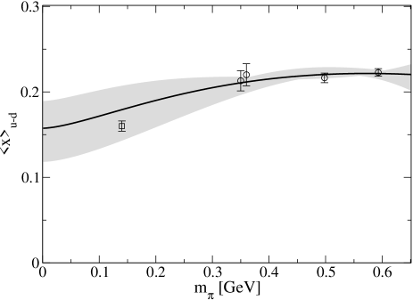
Figure 3: “Fit I” of the ${\cal O}(p^{2})$ result of Eq.(28) to the (preliminary) LHPC lattice data of ref.[24]. The corresponding parameters are given in Table 2. Note that the phenomenological value at physical pion mass was not included in the fit. The grey band shown indicates the estimate of possible ${\cal O}(p^{3})$ corrections as discussed in the text.

	Fit I (4 points - 2 parameter)	Fit II (6+1 points - 3 parameter)
$a_{2,0}^{v}$	0.157 $\pm$ 0.006	0.141 $\pm$ 0.0057
$\Delta a_{2,0}^{v}$	0.210 (fixed)	0.144 $\pm$ 0.034
$c_{8}^{r}$(1GeV)	-0.283 $\pm$ 0.011	-0.213 $\pm$ 0.03

Table 2: Values of the couplings resulting from the two fits to the LHPC lattice data for $\langle x\rangle_{u-d}$. The errors shown are only statistical and do neither include uncertainties from possible higher order corrections in ChEFT nor from systematic uncertainties connected with the lattice simulation.

We note that the mechanism of the downward-bending at small quark-masses in $A_{2,0}^{v}(0)$ found in Eq.(28) is quite different from what has been discussed so far in the literature within the non-relativistic HBChPT framework (e.g. see ref.[35]). In order to demonstrate this we truncate Eq.(28) at $1/(16\pi^{2}F_{\pi}^{2}M_{0})$ to obtain the exact ${\cal O}(p^{2})$ HBChPT result of refs.[36, 37]:

$$A_{2,0}^{v}(0)|_{HBChPT}^{p^{2}} = a_{2,0}^{v}\bigg{\{}1-\frac{m_{\pi}^{2}}{(4\pi F_{\pi})^{2}}\bigg{(}2g_{A}^{2}+(3g_{A}^{2}+1)\log\frac{m_{\pi}^{2}}{\lambda^{2}}\bigg{)}\bigg{\}}+4m_{\pi}^{2}\frac{c_{8}^{(r)}(\lambda)}{M_{0}^{2}}$$ (30)

$$\quad\quad+{\cal O}\left(\frac{1}{16\pi^{2}F_{\pi}^{2}M_{0}}\right).$$

As already stated in the Introduction, the covariant BChPT scheme used in this work is able to reproduce exactly the corresponding non-relativistic HBChPT result at the same order by the appropriate truncation in $1/(16\pi^{2}F_{\pi}^{2}M_{0})$.

Fit I is certainly constricted by the assumption that we use the physical value of $\langle\Delta x\rangle_{u-d}^{phen.}\approx 0.21$ for the coupling $\Delta a_{2,0}^{v}$, which presumably takes a value in the chiral limit a bit smaller than the phenomenological value at the physical point [29]. Furthermore, in order to also compare the ${\cal O}(p^{2})$ HBChPT result of Eq.(30) with the ${\cal O}(p^{2})$ covariant BChPT result of Eq.(28) we perform a second fit: We fit the covariant expression for $\langle x\rangle_{u-d}$ of Eq.(28) again to the LHPC lattice data, this time, however, we constrain the coupling $\Delta a_{2,0}^{v}$ in such a way, that the resulting chiral extrapolation curve reproduces the phenomenological value of $\langle x\rangle_{u-d}^{phen.}=0.160\pm 0.006$ [26] exactly for physical quark masses. The parameter values for this Fit II are again given in table 2, whereas the resulting chiral extrapolation curve of the covariant ${\cal O}(p^{2})$ expression of Eq.(28) is shown as the solid line in Fig.4. First, we would like to emphasize that the curve looks very reasonable, connecting the physical point with the lattice data of the LHPC collaboration in a smooth fashion. Second, we note that the resulting values for the couplings $a_{2,0}^{v},\,\Delta a_{2,0}^{v}$ underlying this curve are very reassuring, indicating that both $\langle x\rangle_{u-d}$ and $\langle\Delta x\rangle_{u-d}$ are slightly smaller in the chiral limit than at the physical point! Likewise, the unknown quark-mass insertion $c_{8}^{(r)}$ contributes in a strength just as expected from natural sizes estimates. For the comparison with HBChPT we now utilize the very same values for $a_{2,0}^{v}$ and $c_{8}^{(r)}$ of Fit II as given in table 2. The resulting curve based on the ${\cal O}(p^{2})$ HBChPT formula of Eq.(30) is shown as the dashed curve in Fig.4. One observes that this leading-one-loop HBChPT expression agrees with the covariant result between the chiral limit and the physical point, but is not able to extrapolate on towards the lattice data. However, we note that all our numerical comparisons with HBChPT results shown in the figures of section 4 and 5 are based on the assumption that the D=2 fit values found in tables 2 and 3 are already reliable estimates of the true, correct values of these couplings in low energy QCD. Clearly, the shown HBChPT curves might have to be revised if future D=3 analyses [32] lead to substantially different numerical values for these couplings. The true range of applicability of HBChPT versus covariant BChPT can only be determined, once the stability of the employed couplings is guaranteed. A study of higher order effects is therefore essential also in this respect. Ideally we would like to reanalyse the results of Fit II by first fixing the couplings from a fit of the HBChPT formula of Eq.(30) and then study the resulting $\mathcal{O}(p^{2})$ BChPT curve for this observable. However, a fit to the present set of lattice data shown in Fig.3 leads to a curve that is not compatible with the 2 lightest lattice points and lies significantly below the grey band shown in Fig.3—even down to the chiral limit. We will study this issue further in ref.[32].

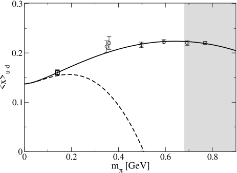
Figure 4: “Fit II” of the ${\cal O}(p^{2})$ BChPT result of Eq.(28) to the (preliminary) LHPC lattice data of ref.[24] and to the physical point (solid line). The corresponding fit-parameters are given in table 2. The dashed curve shown corresponds to ${\cal O}(p^{2})$ result in the HBChPT truncation (see Eq.(30)). The shaded area indicates the region where one does not expect that ChEFT can provide a trustworthy chiral extrapolation function due to the large pion-masses involved, albeit the covariant ${\cal O}(p^{2})$ result does not signal any breakdown in this region.

Keeping these caveats in mind, at this point we conclude that the smooth extrapolation behaviour of the covariant ${\cal O}(p^{2})$ BChPT expression for $\langle x\rangle_{u-d}$ of Eq.(28) between the chiral limit and the region of present lattice QCD data is due to an infinite tower of $\left(\frac{m_{\pi}}{M_{0}}\right)^{n}$ terms. According to our analysis the chiral curvature resulting from the logarithm of Eq.(30) governing the leading-non-analytic quark-mass behaviour of this moment is not responsible for the rising behaviour of the chiral extrapolation function, as had been hypothesized in ref.[35]. It will be interesting to see how well our ${\cal O}(p^{2})$ BChPT extrapolation formula for $\langle x\rangle_{u-d}$ will perform, once the new lattice QCD data from dynamical simulations at small quark masses for moments of GPDs become available [39].
Finally, we are discussing the ${\cal O}(p^{2})$ BChPT results at $t=0$ for the remaining two generalized isovector form factors of the nucleon at twist-2 level. One obtains

$$B_{2,0}^{v}(t=0) = b_{2,0}^{v}\frac{M_{N}(m_{\pi})}{M_{0}}+\frac{a_{2,0}^{v}\,g_{A}^{2}m_{\pi}^{2}}{(4\pi F_{\pi})^{2}}\,\bigg{\{}\bigg{(}3+\log\frac{m_{\pi}^{2}}{M_{0}^{2}}\bigg{)}-\frac{m_{\pi}^{2}}{M_{0}^{2}}\bigg{(}2+3\log\frac{m_{\pi}^{2}}{M_{0}^{2}}\bigg{)}$$ (31)

$$+\frac{m_{\pi}^{4}}{M_{0}^{4}}\log\frac{m_{\pi}^{2}}{M_{0}^{2}}-\frac{2m_{\pi}}{\sqrt{4M_{0}^{2}-m_{\pi}^{2}}}\bigg{(}5-5\frac{m_{\pi}^{2}}{M_{0}^{2}}+\frac{m_{\pi}^{4}}{M_{0}^{4}}\bigg{)}\arccos\bigg{(}\frac{m_{\pi}}{2M_{0}}\bigg{)}\bigg{\}}+{\cal O}(p^{3}),$$

$$C_{2,0}^{v}(t=0) = c_{2,0}^{v}\frac{M_{N}(m_{\pi})}{M_{0}}+\frac{a_{2,0}^{v}g_{A}^{2}m_{\pi}^{2}}{12(4\pi F_{\pi})^{2}}\,\bigg{\{}-1+2\frac{m_{\pi}^{2}}{M_{0}^{2}}\bigg{(}1+\log\frac{m_{\pi}^{2}}{M_{0}^{2}}\bigg{)}$$ (32)

$$-\frac{m_{\pi}^{4}}{M_{0}^{4}}\log{\frac{m_{\pi}^{2}}{M_{0}^{2}}}+\frac{2m_{\pi}}{\sqrt{4M_{0}^{2}-m_{\pi}^{2}}}\bigg{(}2-4\frac{m_{\pi}^{2}}{M_{0}^{2}}+\frac{m_{\pi}^{4}}{M_{0}^{4}}\bigg{)}\arccos\bigg{(}\frac{m_{\pi}}{2M_{0}}\bigg{)}\bigg{\}}+{\cal O}(p^{3}).$$

As one can easily observe, one encounters plenty of non-analytic terms and even chiral logarithms in these covariant ${\cal O}(p^{2})$ BChPT results. However, we note that in the HBChPT limit to the same chiral order ${\cal O}(p^{2})$ one would only obtain the chiral limit values $b_{2,0}^{v},\,c_{2,0}^{v}$, nothing else [41]. E.g. the chiral logarithms calculated in ref.[14] for $B_{2,0}^{v}(t=0),\,C_{2,0}^{v}(t=0)$ would only show up in a full ${\cal O}(p^{3})$, respectively ${\cal O}(p^{4})$ BChPT calculation of the generalized form factors. From the viewpoint of power-counting in BChPT they are to be considered part of the higher order corrections to the full ${\cal O}(p^{2})$ results given in Eqs.(31,32).

Unfortunately, at this point no information from experiment exists for these two structure quantities of the nucleon. From phenomenology one would expect that $B_{2,0}^{v}(t=0)$ has a “large” positive value at $m_{\pi}=140$ MeV, as it corresponds to the next-higher moment of the isovector Pauli form factor $F_{2}^{v}(t=0)\equiv\kappa_{v}=3.7$ n.m. (Compare Eq.(5) and Eq.(3) at $\xi=0$). Lattice QCD analyses seem to support this expectation [22, 23, 24]. In contrast, the value of $C_{2,0}^{v}(t=0)$ cannot be estimated from information known about nucleon form factors. State-of-the-art lattice QCD analyses (e.g. see ref.[24]) suggest that it is consistent with zero. In Fig.5 we have indicated how the corresponding extrapolation curves based upon this information might look like. We are looking forward to a combined analysis of Eqs(31,32) and the new lattice QCD data from dynamical simulations at small quark-masses [39] extrapolated to $t=0$, which will shed new light onto this new domain of nucleon structure physics! As a caveat we note that in both form factors we would see a dominant influence of the quark-mass dependence stemming from the kinematical factor $M_{N}(m_{\pi})$ in Eq.(LABEL:defv), if their corresponding chiral limit values $b_{2,0}^{v},\,c_{2,0}^{v}\neq 0$. A further observation is that the uncertainties connected with possible higher order corrections from ${\cal O}(p^{3})$ could already become substantial for pion masses around 300 MeV. For both quantities they can be estimated via ${\cal O}(p^{3})\sim\delta_{B,C}\frac{m_{\pi}^{2}M_{N}(m_{\pi})}{\Lambda_{\chi}^{2}M_{0}}$ where $-1<\delta_{B,C}<1$. In order to ultimately test the stability of the results in Eqs.(31,32) it will be very useful to extend this analysis to next-to-leading one-loop order [32].

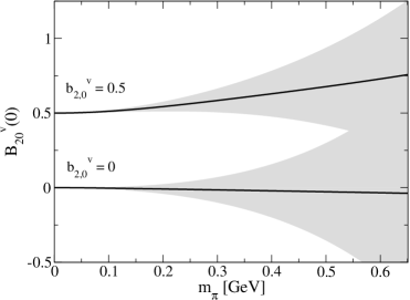
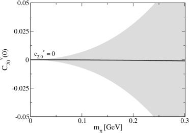
Figure 5: Quark-mass dependence of the isovector moments $B_{2,0}^{v}(t=0)$ and $C_{2,0}^{v}(t=0)$. In $B_{2,0}^{v}(t=0)$ we have varied the (unknown) chiral limit value $b_{2,0}^{v}$ between $0$ and $+0.5$, as lattice analyses [22, 23, 24] suggest that this moment has a large positive value. For the chiral limit value $c_{2,0}^{v}$ of $C_{2,0}^{v}(t=0)$ we have chosen the value 0, as preliminary lattice QCD analyses suggest that this moment is consistent with zero [24]. The grey bands shown indicate the size of possible higher order corrections to these ${\cal O}(p^{2})$ results.

4.2 The slopes of the generalized isovector Form Factors

In order to discuss the generalized isovector form factors $A_{2,0}^{v}(t),\,B_{2,0}^{v}(t),\,C_{2,0}^{v}(t)$ at non-zero values of $t$, we first want to analyze their slopes $\rho_{X}$, defined via

$$X_{2,0}^{v}(t) = X_{2,0}^{v}(0)+\rho_{X}^{v}\,t\;+{\cal O}(t^{2});\quad\quad X=A,B,C.$$ (33)

To ${\cal O}(p^{2})$ in BChPT we find

$$\rho_{A}^{v} = \frac{c_{12}}{M_{0}^{2}}-\frac{a_{2,0}^{v}g_{A}^{2}}{6(4\pi F_{\pi})^{2}}\,\frac{m_{\pi}^{2}}{(4M_{0}^{2}-m_{\pi}^{2})}\,\bigg{\{}26+8\log\frac{m_{\pi}^{2}}{M_{0}^{2}}-\frac{m_{\pi}^{2}}{M_{0}^{2}}\bigg{(}30+32\log\frac{m_{\pi}^{2}}{M_{0}^{2}}\bigg{)}$$ (34)

$$+\frac{m_{\pi}^{4}}{M_{0}^{4}}\bigg{(}6+\frac{39}{2}\log\frac{m_{\pi}^{2}}{M_{0}^{2}}\bigg{)}-3\frac{m_{\pi}^{6}}{M_{0}^{6}}\log\frac{m_{\pi}^{2}}{M_{0}^{2}}$$

$$-\frac{m_{\pi}}{\sqrt{4M_{0}^{2}-m_{\pi}^{2}}}\bigg{(}90-130\frac{m_{\pi}^{2}}{M_{0}^{2}}+51\frac{m_{\pi}^{4}}{M_{0}^{4}}-6\frac{m_{\pi}^{6}}{M_{0}^{6}}\bigg{)}\arccos\bigg{(}\frac{m_{\pi}}{2M_{0}}\bigg{)}\bigg{\}}+\frac{m_{\pi}}{\Lambda_{\chi}^{2}M_{0}}\delta_{A}^{t},$$

$$\rho_{B}^{v} = \frac{a_{2,0}^{v}g_{A}^{2}}{18(4\pi F_{\pi})^{2}}\,\frac{1}{(4M_{0}^{2}-m_{\pi}^{2})}\bigg{\{}4M_{0}^{2}+m_{\pi}^{2}\bigg{(}83+24\log\frac{m_{\pi}^{2}}{M_{0}^{2}}\bigg{)}-114\frac{m_{\pi}^{4}}{M_{0}^{2}}\bigg{(}1+\log\frac{m_{\pi}^{2}}{M_{0}^{2}}\bigg{)}$$ (35)

$$+\frac{m_{\pi}^{6}}{M_{0}^{4}}\bigg{(}24+75\log\frac{m_{\pi}^{2}}{M_{0}^{2}}\bigg{)}-12\frac{m_{\pi}^{8}}{M_{0}^{6}}\log\frac{m_{\pi}^{2}}{M_{0}^{2}}-\frac{6m_{\pi}^{3}}{\sqrt{4M_{0}^{2}-m_{\pi}^{2}}}\bigg{(}50-80\frac{m_{\pi}^{2}}{M_{0}^{2}}+33\frac{m_{\pi}^{4}}{M_{0}^{4}}-4\frac{m_{\pi}^{6}}{M_{0}^{6}}\bigg{)}$$

$$\times\arccos\bigg{(}\frac{m_{\pi}}{2M_{0}}\bigg{)}\bigg{\}}+\delta_{B}^{t}\,\frac{M_{N}(m_{\pi})}{\Lambda_{\chi}^{2}M_{0}},$$

$$\rho_{C}^{v} = \frac{a_{2,0}^{v}g_{A}^{2}}{180(4\pi F_{\pi})^{2}}\frac{1}{(4M_{0}^{2}-m_{\pi}^{2})}\bigg{\{}4M_{0}^{2}-13m_{\pi}^{2}+12\frac{m_{\pi}^{4}}{M_{0}^{2}}\bigg{(}4+3\log\frac{m_{\pi}^{2}}{M_{0}^{2}}\bigg{)}$$ (36)

$$-3\frac{m_{\pi}^{6}}{M_{0}^{4}}\bigg{(}4+11\log\frac{m_{\pi}^{2}}{M_{0}^{2}}\bigg{)}+6\frac{m_{\pi}^{8}}{M_{0}^{6}}\log\frac{m_{\pi}^{2}}{M_{0}^{2}}+\frac{6m_{\pi}^{3}}{\sqrt{4M_{0}^{2}-m_{\pi}^{2}}}\bigg{(}10-30\frac{m_{\pi}^{2}}{M_{0}^{2}}+15\frac{m_{\pi}^{4}}{M_{0}^{4}}-2\frac{m_{\pi}^{6}}{M_{0}^{6}}\bigg{)}$$

$$\times\arccos\bigg{(}\frac{m_{\pi}}{2M_{0}}\bigg{)}\bigg{\}}+\delta_{C}^{t}\,\frac{M_{N}(m_{\pi})}{\Lambda_{\chi}^{2}M_{0}}.$$

The parameters $\delta_{A}^{t},\,\delta_{B}^{t},\,\delta_{C}^{t}$ are not part of the covariant $\mathcal{O}(p^{2})$ result. They are only given to indicate the size of possible higher order corrections from ${\cal O}(p^{3})$. A numerical analysis of the formulae given above suggests that the size of pion-cloud contributions to the slopes of the generalized isovector form factors is very small! The physics governing the size of these objects seems to be hidden in the counterterm contributions $c_{12},\,\delta_{B}^{t},\,\delta_{C}^{t}$ which dominate numerically when assuming natural size estimates $-1<c_{12},\,\delta_{B}^{t},\,\delta_{C}^{t}<+1$. We note that this situation reminds us of the isoscalar Dirac and Pauli form factors of the nucleon $F_{1}^{s}(t),\,F_{2}^{s}(t)$, where the t-dependence in SU(2) ChEFT calculations is also dominated by counterterms (e.g. see the discussion in ref.[3]).

Finally, truncating the covariant results of Eqs.(34-36) at $1/(16\pi^{2}F_{\pi}^{2}M_{0})$ we obtain the (trivial) HBChPT expressions to ${\cal O}(p^{2})$:

$$\rho_{A}^{v} = \frac{c_{12}}{M_{0}^{2}}+{\cal O}(p^{3}),$$ (37)

$$\rho_{B}^{v} = 0+{\cal O}(p^{3}),$$ (38)

$$\rho_{C}^{v} = 0+{\cal O}(p^{3}).$$ (39)

The non-zero slope results found in the HBChPT calculations of refs.[15, 16] are therefore of higher order from the point of view of our powercounting. Most of them can already be added systematically to our covariant ${\cal O}(p^{2})$ results of Eqs.(34-36) at ${\cal O}(p^{3})$ [32].

4.3 Generalized isovector Form Factors of the Nucleon

In this subsection we present the full t-dependence of the (generalized) isovector form factors of a nucleon to ${\cal O}(p^{2})$ in BChPT. We note that for all three form factors at this order only diagram c) of Fig.1 gives a non-zero contribution at finite values of $t$—the resulting expressions at this order are therefore quite simple:

$$A_{2,0}^{v}(t) = A_{2,0}^{v}(0)+\frac{a_{2,0}^{v}g_{A}^{2}}{192\pi^{2}F_{\pi}^{2}}F_{2,0}^{v}(t)+\frac{c_{12}}{M_{0}^{2}}\,t+\mathcal{O}(p^{3}),$$ (40)

with

$$F_{2,0}^{v}(t) = t-\frac{2m_{\pi}^{3}\left(50M_{0}^{4}-43m_{\pi}^{2}M_{0}^{2}+8m_{\pi}^{4}\right)}{M_{0}^{4}\sqrt{4M_{0}^{2}-m_{\pi}^{2}}}\arccos{\left(\frac{m_{\pi}}{2M_{0}}\right)}$$

$$+\int_{-\frac{1}{2}}^{\frac{1}{2}}\,du\Bigg{\{}\frac{2m_{\pi}^{3}M_{0}^{2}}{\tilde{M}^{8}\sqrt{4\tilde{M}^{2}-m_{\pi}^{2}}}\left[-10\tilde{M}^{6}+\left(17m_{\pi}^{2}+60M_{0}^{2}\right)\tilde{M}^{4}-4m_{\pi}^{2}\left(m_{\pi}^{2}+15M_{0}^{2}\right)\tilde{M}^{2}\right.$$

$$\left.+12m_{\pi}^{4}M_{0}^{2}\right]\arccos{\left(\frac{m_{\pi}}{2\tilde{M}}\right)}+\frac{2\left(M_{0}^{2}-\tilde{M}^{2}\right)}{M_{0}^{2}\tilde{M}^{6}}\left[12m_{\pi}^{4}M_{0}^{4}+2m_{\pi}^{2}\left(4m_{\pi}^{2}-9M_{0}^{2}\right)M_{0}^{2}\tilde{M}^{2}\right.$$

$$\left.+\left(m_{\pi}^{2}-2M_{0}^{2}\right)\left(8m_{\pi}^{2}+M_{0}^{2}\right)\tilde{M}^{4}\right]+\frac{2M_{0}^{2}}{\tilde{M}^{8}}\left[2\tilde{M}^{8}+3m_{\pi}^{2}\left(3m_{\pi}^{2}+4M_{0}^{2}\right)\tilde{M}^{4}\right.$$

$$\left.-4m_{\pi}^{4}\left(m_{\pi}^{2}+9M_{0}^{2}\right)\tilde{M}^{2}+12m_{\pi}^{6}M_{0}^{2}\right]\log{\left(\frac{\tilde{M}}{M_{0}}\right)}+\frac{2m_{\pi}^{2}}{M_{0}^{4}\tilde{M}^{8}}\left[m_{\pi}^{4}\left(-12M_{0}^{8}+4\tilde{M}^{2}M_{0}^{6}\right.\right.$$

$$\left.\left.+8\tilde{M}^{8}\right)+9m_{\pi}^{2}\tilde{M}^{2}\left(4M_{0}^{8}-\tilde{M}^{2}M_{0}^{6}-3\tilde{M}^{6}M_{0}^{2}\right)+12M_{0}^{4}\tilde{M}^{4}\left(\tilde{M}^{4}-M_{0}^{4}\right)\right]\log{\left(\frac{m_{\pi}}{M_{0}}\right)}\Bigg{\}},$$

and $\tilde{M}^{2}=M_{0}^{2}+\left(u^{2}-\frac{1}{4}\right)t$. Note that $F_{2,0}^{v}(t=0)\equiv 0$, whereas $A_{2,0}^{v}(0)$ has been discussed in section 4.1. A conservative estimate for the size of possible higher order corrections indicated in Eq.(40) can be obtained via $\mathcal{O}(p^{3})\sim\delta_{A}\,\frac{m_{\pi}^{3}}{\Lambda_{\chi}^{2}M_{0}}+\delta_{A}^{t}\,\frac{m_{\pi}}{\Lambda_{\chi}^{2}M_{0}}\,t$, as discussed in the two previous subsections. For the remaining two (generalized) isovector form factors we obtain

$$B_{2,0}^{v}(t) = b_{2,0}^{v}\,\frac{M_{N}(m_{\pi})}{M_{0}}+\frac{a_{2,0}^{v}g_{A}^{2}M_{0}^{2}}{48\pi^{2}F_{\pi}^{2}}\int_{-\frac{1}{2}}^{\frac{1}{2}}\!\frac{du}{\tilde{M}^{8}}\Bigg{\{}\left(M_{0}^{2}-\tilde{M}^{2}\right)\tilde{M}^{6}+9m_{\pi}^{2}M_{0}^{2}\tilde{M}^{4}$$ (42)

$$-6m_{\pi}^{4}M_{0}^{2}\tilde{M}^{2}+6m_{\pi}^{2}M_{0}^{2}\left(m_{\pi}^{4}-3m_{\pi}^{2}\tilde{M}^{2}+\tilde{M}^{4}\right)\log{\frac{m_{\pi}}{\tilde{M}}}$$

$$-\frac{6m_{\pi}^{3}M_{0}^{2}}{\sqrt{4\tilde{M}^{2}-m_{\pi}^{2}}}\bigg{[}m_{\pi}^{4}-5m_{\pi}^{2}\tilde{M}^{2}+5\tilde{M}^{4}\bigg{]}\arccos{\left(\frac{m_{\pi}}{2\tilde{M}}\right)}\Bigg{\}}$$

$$+\delta_{B}\,\frac{m_{\pi}^{2}M_{N}(m_{\pi})}{\Lambda_{\chi}^{2}M_{0}}+\delta_{B}^{t}\,\frac{M_{N}(m_{\pi})}{\Lambda_{\chi}^{2}M_{0}}\,t,$$

$$C_{2,0}^{v}(t) = c_{2,0}^{v}\frac{M_{N}(m_{\pi})}{M_{0}}+\frac{a_{2,0}^{v}g_{A}^{2}M_{0}^{2}}{48\pi^{2}F_{\pi}^{2}}\int_{-\frac{1}{2}}^{\frac{1}{2}}\frac{du\,u^{2}}{\tilde{M}^{8}}\Bigg{\{}2\left(M_{0}^{2}-\tilde{M}^{2}\right)\tilde{M}^{6}-3m_{\pi}^{2}M_{0}^{2}\tilde{M}^{4}$$ (43)

$$+6m_{\pi}^{4}M_{0}^{2}\tilde{M}^{2}-6m_{\pi}^{4}M_{0}^{2}\left(m_{\pi}^{2}-2\tilde{M}^{2}\right)\log{\frac{m_{\pi}}{\tilde{M}}}$$

$$+\frac{6m_{\pi}^{3}M_{0}^{2}}{\sqrt{4\tilde{M}^{2}-m_{\pi}^{2}}}\bigg{[}m_{\pi}^{4}-4m_{\pi}^{2}\tilde{M}^{2}+2\tilde{M}^{4}\bigg{]}\arccos{\left(\frac{m_{\pi}}{2\tilde{M}}\right)}\Bigg{\}}$$

$$+\delta_{C}\,\frac{m_{\pi}^{2}M_{N}(m_{\pi})}{\Lambda_{\chi}^{2}M_{0}}+\delta_{C}^{t}\,\frac{M_{N}(m_{\pi})}{\Lambda_{\chi}^{2}M_{0}}\,t.$$

The parameters $\delta_{B},\,\delta_{C},\,\delta_{B}^{t},\,\delta_{C}^{t}$ have been inserted to study the possible corrections of higher orders to our ${\cal O}(p^{2})$ results. Varying these parameters between -1 and +1 we conclude that a full ${\cal O}(p^{3})$ calculation is required, before we want to make any strong claims regarding the t-dependence of $B_{2,0}^{v}(t)$ and $C_{2,0}^{v}(t)$ beyond the linear t-dependence discussed in the previous subsection. On the other hand, the predicted t-dependence of the form factor $A_{2,0}^{v}(t)$ of Eq.(40) appears to be more reliable at this order, as possible higher order contributions only affect terms beyond the leading linear dependence in t.

5 Generalized isoscalar Form Factors in ${\cal O}(p^{2})$ BChPT

5.1 Moments of the isoscalar GPDs at $t=0$

To ${\cal O}(p^{2})$ in 2-flavor covariant BChPT the only non-zero loop contributions to the isoscalar moment $A_{2,0}^{s}(t=0)$ (see Eq.(10)) arise from diagrams c) and e) in Fig.1. One obtains

$$A_{2,0}^{s}(0) = \langle x\rangle_{u+d}$$ (44)

$$= a_{2,0}^{s}+4m_{\pi}^{2}\frac{c_{9}}{M_{0}^{2}}-\frac{3a_{2,0}^{s}g_{A}^{2}m_{\pi}^{2}}{16\pi^{2}F_{\pi}^{2}}\Bigg{[}\frac{m_{\pi}^{2}}{M_{0}^{2}}+\frac{m_{\pi}^{2}}{M_{0}^{2}}\left(2-\frac{m_{\pi}^{2}}{M_{0}^{2}}\right)\log{\left(\frac{m_{\pi}}{M_{0}}\right)}$$

$$+\frac{m_{\pi}}{\sqrt{4M_{0}^{2}-m_{\pi}^{2}}}\left(2-4\frac{m_{\pi}^{2}}{M_{0}^{2}}+\frac{m_{\pi}^{4}}{M_{0}^{4}}\right)\arccos{\left(\frac{m_{\pi}}{2M_{0}}\right)}\Bigg{]}+{\cal O}(p^{3}).$$

Eq.(44) should provide a similarly successful chiral extrapolation function for $\langle x\rangle_{u+d}$ as the covariant ${\cal O}(p^{2})$ BChPT result of Eq.(28) did for the LHPC lattice data for $\langle x\rangle_{u-d}$ in section 4.1. The uncertainty arising from higher orders can be estimated to scale as ${\cal O}(p^{3})\sim\delta_{A}^{0}\frac{m_{\pi}^{3}}{\Lambda_{\chi}^{2}M_{0}}$, where $\delta_{A}^{0}$ should be a number between $-1,\ldots,+1$, according to natural size estimates. We note that the coupling $\Delta a_{2,0}^{v}$, which played an essential role in the chiral extrapolation function of $\langle x\rangle_{u-d}$, is not present in the quark-mass dependence of the isoscalar moment $\langle x\rangle_{u+d}$. The resulting chiral extrapolation function is therefore presumably quite different from the one in the isovector channel. The absence of a chiral logarithm $\sim m_{\pi}^{2}\log m_{\pi}$ in $\langle x\rangle_{u+d}$ (compare Eq.(30) and Eq.(44)) presumably will only lead to a difference in the chiral extrapolation functions between the isovector and the isoscalar moment for values $m_{\pi}<140$ MeV.

Note that from Eq.(44) in the limit $1/(16\pi^{2}F_{\pi}^{2}M_{0})\rightarrow 0$ we reproduce the leading HBChPT result for $\langle x\rangle_{u+d}$ of ref.[36], which found a complete cancellation of the non-analytic quark-mass dependent terms in this channel (in the static limit):

$$A_{2,0}^{s}(0)|_{HBChPT}^{p^{2}} = a_{2,0}^{s}+4m_{\pi}^{2}\frac{c_{9}}{M_{0}^{2}}+{\cal O}(1/(16\pi^{2}F_{\pi}^{2}M_{0})).$$ (45)

The coupling $c_{9}$ is therefore scale independent (in dimensional regularization) and constitutes the leading correction to the chiral limit value $a_{2,0}^{s}$ of $\langle x\rangle_{u+d}$.

At $t=0$ we also find non-trivial results for the two other generalized isoscalar form factors of the nucleon to this order in the calculation

$$B_{2,0}^{s}(0) = b_{2,0}^{s}\,\frac{M_{N}(m_{\pi})}{M_{0}}-\frac{3\,a_{2,0}^{s}\,g_{A}^{2}m_{\pi}^{2}}{(4\pi F_{\pi})^{2}}\,\bigg{\{}\bigg{(}3+\log\frac{m_{\pi}^{2}}{M_{0}^{2}}\bigg{)}-\frac{m_{\pi}^{2}}{M_{0}^{2}}\bigg{(}2+3\log\frac{m_{\pi}^{2}}{M_{0}^{2}}\bigg{)}$$ (46)

$$+\frac{m_{\pi}^{4}}{M_{0}^{4}}\log\frac{m_{\pi}^{2}}{M_{0}^{2}}-\frac{2m_{\pi}}{\sqrt{4M_{0}^{2}-m_{\pi}^{2}}}\bigg{(}5-5\frac{m_{\pi}^{2}}{M_{0}^{2}}+\frac{m_{\pi}^{4}}{M_{0}^{4}}\bigg{)}\arccos\bigg{(}\frac{m_{\pi}}{2M_{0}}\bigg{)}\bigg{\}}$$

$$+\delta_{B}^{0}\frac{m_{\pi}^{2}M_{N}(m_{\pi})}{\Lambda_{\chi}^{2}M_{0}},$$

$$C_{2,0}^{s}(0) = c_{2,0}^{s}\,\frac{M_{N}(m_{\pi})}{M_{0}}-\frac{\,a_{2,0}^{s}g_{A}^{2}m_{\pi}^{2}}{4(4\pi F_{\pi})^{2}}\,\bigg{\{}-1+2\frac{m_{\pi}^{2}}{M_{0}^{2}}\bigg{(}1+\log\frac{m_{\pi}^{2}}{M_{0}^{2}}\bigg{)}-\frac{m_{\pi}^{4}}{M_{0}^{4}}\log\frac{m_{\pi}^{2}}{M_{0}^{2}}$$ (47)

$$+\frac{2m_{\pi}}{\sqrt{4M_{0}^{2}-m_{\pi}^{2}}}\bigg{(}2-4\frac{m_{\pi}^{2}}{M_{0}^{2}}+\frac{m_{\pi}^{4}}{M_{0}^{4}}\bigg{)}\arccos\bigg{(}\frac{m_{\pi}}{2M_{0}}\bigg{)}\bigg{\}}+\delta_{C}^{0}\frac{m_{\pi}M_{N}(m_{\pi})}{\Lambda_{\chi}^{2}}.$$

Note that additional chiral logarithms appear in the HBChPT calculations of refs.[15, 16], e.g. a term $\leavevmode\nobreak\ b_{20}^{s}m_{\pi}^{2}\log{m_{\pi}}$ entering the analogue of Eq.(46). According to the chiral power-counting formula Eq.(26) such a term only starts to appear at $\sim\mathcal{O}(p^{3})$, and is therefore not present in our $\mathcal{O}(p^{2})$ calculation. We have added the parameters $\delta_{B}^{0},\,\delta_{C}^{0}$ “by hand” to our covariant $\mathcal{O}(p^{2})$ results Eqs.(46) and (47) in order to indicate possible effects of higher order (i.e. ${\cal O}(p^{3})$) corrections. Presumably they take on values $-1,\ldots,+1$. Note that our ${\cal O}(p^{2})$ BChPT prediction for $C_{2,0}^{s}(0)$ is strongly affected by possible corrections from higher orders. This is due to the fact that one only receives a non-zero result for this form factor starting at ${\cal O}(p^{2})$—the order we are working in. Eq.(47) should therefore only be considered to provide a rough estimate for the quark mass dependence of this form factor at $t=0$. For a true quantitative analysis of its chiral extrapolation behaviour the complete ${\cal O}(p^{3})$ corrections should first be added [32].

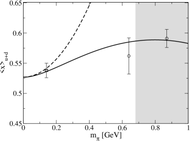
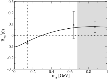
Figure 6: Solid lines: The quark mass dependence of the $\mathcal{O}(p^{2})$ BChPT result for $\langle x\rangle_{u+d}$ of Eq.(44) and $B_{2,0}^{s}(0)$ of Eq.(46). The three unknown parameters resulting from a combined fit to the shown QCDSF data of ref.[22] and to the phenomenological value for $\langle x\rangle_{u+d}$ [26] are given in table 3. At the physical point we obtain $B_{2,0}^{s}=-0.056\pm 0.016$, with the shown error only being statistical. Due to the poor data situation with its unknown systematic errors, however, these results should only be considered as a rough estimate of the true quark-mass dependence. The dashed line corresponds to the respective HBChPT result at this order.

Unfortunately, the (published) lattice QCD data base for $\langle x\rangle_{u+d}$ and $B_{2,0}^{s}(t\rightarrow 0)$ is quite sparse for small values of the pion mass. In order to obtain a rough estimate of the chiral extrapolation functions resulting from Eqs.(44,46) we have to resort to (quenched) data of the QCDSF collaboration in ref.[22]. Performing a combined fit of Eqs.(44,46) to the lattice data shown in Fig.6 and including the phenomenological value of $\langle x\rangle_{u+d}\sim 0.54$ [26] we obtain the two solid curves shown in Fig.6. The resulting parameters of the fit are given in table 3. Interestingly, despite the large quark-masses and the huge error bars in the data of ref.[22] we obtain reasonable chiral extrapolation curves with natural size couplings. The analysis of the QCDSF data in combination with the physical value for $\langle x\rangle_{u+d}$ suggests that the chiral limit value of this isoscalar PDF-moment is smaller than the value at the physical point, leading to a monotonically rising chiral extrapolation function as shown in the left panel of Fig.6. It will be very interesting to observe what values an upcoming analysis of the new LHPC data will find [39] for this moment, as a glance at the preliminary results shown in ref.[24] seems to indicate that for effective pion masses around 300 MeV LHPC finds values for $\langle x\rangle_{u+d}$ which are lower than the physical point. If this observation can be confirmed in the final analysis of the data [39] one would have to conclude that the chiral extrapolation behaviour of $\langle x\rangle_{u+d}$ is truly extraordinary, displaying a minimum for effective pion masses near 300-400 MeV before rising again to larger values for large quark masses.

As a second observation, we would like to note that the value for the generalized form factor $B_{2,0}^{s}(t=0)$ could take on a small negative value at the physical point according to the right panel of Fig.6, albeit with a large uncertainty due to the poor data situation. Because of the small (negative!) value of the isoscalar Pauli form factor $F_{2}^{s}(t=0)\equiv\kappa_{s}=-0.12$ n.m., it is somewhat expected that the next-higher moment will yield a value close to zero. However, Fig.6 now opens the possibility that $B_{2,0}^{s}(t=0)\approx-0.06$ might be as large as 50% of its $F_{2}^{s}(t=0)$ analogue. It will be very interesting to observe whether this feature can be reproduced when the new data of QCDSF and LHPC [39] at small pion mass are analyzed with the help of our ${\cal O}(p^{2})$ BChPT formulae Eqs.(44,46).
Finally, we note again that the true range of applicability of HBChPT versus covariant BChPT (see e.g. the left panel of Fig.(6)) can only be determined, once the stability of the employed couplings is guaranteed, see the similar discussion for $\langle x\rangle_{u-d}$ in section 4.1. A study of higher order effects is therefore essential also in this respect.

$a_{2,0}^{s}$	$b_{2,0}^{s}$	$c_{9}$	$\delta_{A}^{0},\,\delta_{B}^{0}$	$\langle x\rangle_{u+d}^{phen.}(\mu=2$GeV$)$
$0.527\pm 0.007$	$-0.103\pm 0.016$	$0.147\pm 0.002$	$0$ (fixed)	$0.538\pm 0.012$ (fixed)

Table 3: The values for the three tensor coupling constants entering $A_{2,0}^{s}(t)$ and $B_{2,0}^{s}(t)$ at order $p^{2}$ as extracted from a combined fit to the lattice points for $A_{2,0}^{s}(0)$ and $B_{2,0}^{s}(0)$ [22] shown in Fig.6 and to the physical point of $A_{2,0}^{s}(t=0,m_{\pi}=0.14$ GeV$)\equiv\langle x\rangle_{u+d}^{phen.}$. Note that we have obtained a small negative value for $b_{2,0}^{s}$. The indicated errors are only statistical and do not reflect the (much larger) systematic uncertainties connected with a fit to the (quenched) lattice data of ref.[22] which e.g. neglect all contributions from disconnected diagrams.

5.2 The contribution of $u-$ and $d-$quarks to the spin of the nucleon

In the past few years a lot of interest in generalized isoscalar form factors of the nucleon has focused on the values of $A_{2,0}^{s},\,B_{2,0}^{s}$ at the point $t=0$, as one can determine the contribution of quarks to the total spin of the nucleon via these two structures [42]:

$$J_{u+d} = \frac{1}{2}\big{[}A_{2,0}^{s}(t=0)+B_{2,0}^{s}(t=0)\big{]}.$$ (48)

To ${\cal O}(p^{2})$ in BChPT we find

$$J_{u+d} = \frac{1}{2}\bigg{\{}a_{2,0}^{s}+b_{2,0}^{s}\,\frac{M_{N}(m_{\pi})}{M_{0}}+\frac{a_{2,0}^{s}m_{\pi}^{2}}{(4\pi F_{\pi})^{2}}\bigg{[}\frac{3g_{A}^{2}m_{\pi}}{\sqrt{4M_{0}^{2}-m_{\pi}^{2}}}\bigg{(}8-6\frac{m_{\pi}^{2}}{M_{0}^{2}}+\frac{m_{\pi}^{4}}{M_{0}^{4}}\bigg{)}\arccos\frac{m_{\pi}}{2M_{0}}$$ (49)

$$-3g_{A}^{2}\bigg{(}3-\frac{m_{\pi}^{2}}{M_{0}^{2}}+\bigg{(}2-4\frac{m_{\pi}^{2}}{M_{0}^{2}}+\frac{m_{\pi}^{4}}{M_{0}^{4}}\bigg{)}\log\frac{m_{\pi}}{M_{0}}\bigg{)}\bigg{]}+4m_{\pi}^{2}\frac{c_{9}}{M_{0}^{2}}\bigg{\}}+{\cal O}(p^{3}).$$

Note that despite the plethora of non-analytic quark-mass dependent terms contained in the ${\cal O}(p^{2})$ BChPT result of Eq.(49), the two chiral logarithms calculated in ref.[13] within the HBChPT framework are not yet contained in our result. Both terms ($\sim a_{(q)\pi},\,b_{(q)N}$ in the notation of ref.[13]) are part of the complete ${\cal O}(p^{3})$ result according to our power-counting and will appear in the calculation of the next order. We further note that the two logarithms of ref.[13] are UV-divergent and are accompanied by a counterterm, whereas the ${\cal O}(p^{2})$ BChPT result of Eq.(49) happens to be UV-finite to the order we are working in. In ref.[13] the authors also reported that the two chiral logarithms (of ${\cal O}(p^{3})$) which they describe presumably are canceled numerically by pion-cloud contributions around an intermediate Delta(1232) state. We can confirm that this possibility exists, as the described Delta contributions also start at ${\cal O}(p^{3})$, assuming a power-counting where the nucleon-Delta mass difference is counted as parameter $\sim p^{1}$ (in the chiral limit) (see ref.[40] for details).

Utilizing the ${\cal O}(p^{2})$ BChPT result of Eq.(49) and the fit parameters of table 3 we obtain a a first estimate for the contribution of $u-$ and $d-$quarks to the spin of a nucleon:

$$J_{u+d}(t=0,\,m_{\pi}=0.14\,\rm{GeV})\approx 0.24\pm 0.05,$$ (50)

which is only 50% of the total spin of the nucleon! Note that we can only give a rough estimate for the error in this determination via assigning a typical size of the input lattice error bars shown in Fig.6 to the extrapolated result, as we are assuming that the true error is dominated by systematic errors in the lattice input to our analysis. (The size of the statistical error read off from the fit of table 3 is $\pm 0.01$ and therefore negligible. The small value of this statistical error is of course heavily influenced by the error assigned to the phenomenological value of $\langle x\rangle_{u+d}$ given in table 3)

Based on the same input (uncertainties) we can also predict the quark-mass dependence of $J_{u+d}$. The result is displayed as the solid line in Fig.7. Note that in contrast to the analysis given in ref.[22], we do not obtain a flat chiral extrapolation function between the lattice data and the physical point. The ${\cal O}(p^{2})$ BChPT analysis suggests that the value at the physical point lies lower than the values obtained in the QCDSF simulation at large quark-masses. However, given the large values of quark-masses and the sizable error-bars in the (quenched) simulation of ref.[22], our extrapolated value for $J_{u+d}$ obviously can only give a first estimate of the true result. We are therefore looking forward to the application of our formula Eq.(49) to the new (fully dynamical) lattice QCD results by QCDSF and LHPC obtained at lower quark-masses with improved statistics [39]. Furthermore, the influence of possible corrections from ${\cal O}(p^{3})$ in Eq.(49) has to be analyzed, before one can obtain a high precision determination of the quark-contribution to the spin of the nucleon from a combined effort of lattice QCD and ChEFT [32].

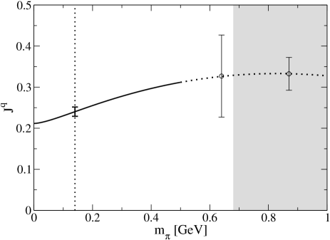
Figure 7: The contribution of $u+d$ quarks to the spin of a nucleon as function of the effective pion mass. The ${\cal O}(p^{2})$ BChPT result shown as the solid line is a prediction of Eq.(49) which utilizes the fit-parameters of table 3. For comparison we have also plotted simulation data from QCDSF [22] in the figure. At the physical point one can read off $J_{u+d}\approx 0.24$. (The error bar shown at the physical point is only statistical and does not reflect any systematic uncertainties.)

5.3 A first glance at the generalized isoscalar form factors of the nucleon

In this section we present the results for the momentum and quark-mass dependence of the generalized form factors of the nucleon for the isoscalar flavour combination $u+d$ at ${\cal O}(p^{2})$ in BChPT. We note that at this order the only non-zero loop contributions to the three isoscalar form factors arise from diagrams c) and e) in Fig.1, as the coupling of the isoscalar tensor field to the nucleon is not affected by chiral rotations. One obtains

$$A_{2,0}^{s}(t) = A_{2,0}^{s}(0)-\frac{a_{2,0}^{s}g_{A}^{2}}{64\pi^{2}F_{\pi}^{2}}F_{2,0}^{s}(t)+\frac{c_{13}}{M_{0}^{2}}\,t+\mathcal{O}(p^{3})\,,$$ (51)

with $A_{2,0}^{s}(0)$ given in Eq.(44) and $F_{2,0}^{s}(t=0)\equiv 0$. Interestingly, to the order we are working here, the $t$-dependence of this isoscalar form factor $A_{2,0}^{s}(t)$ is given by the same function

$$F_{2,0}^{s}(t) = F_{2,0}^{v}(t)+{\cal O}(p^{3}),$$ (52)

that controls its isovector analogue Eq.(LABEL:davt), albeit with larger numerical prefactors (compare Eq.(51) to Eq.(40)). We note that $F_{2,0}^{s}(t)$ does not depend on the scale $\lambda$ of dimensional regularization for the loop diagrams. The chiral coupling $c_{13}$ is therefore also scale-independent, parametrizing the (quark-mass independent) short-distance contributions to the radius/slope of $A_{2,0}^{s}(t)$. The unknown contributions from higher orders in the chiral expansion can be estimated from a calculation of the triangle diagram displayed in Fig.2. Due to the coupling of the tensor field to the (long-range) pion cloud of the nucleon, among all the contributions at the next chiral order this diagram should give the most-important $t$-dependent correction to the covariant ${\cal O}(p^{2})$ result of Eq.(51), resulting in the estimate ${\cal O}(p^{3})\sim\Delta A^{s}_{h.o.}(t,m_{\pi})$. The explicit expression for this function can be found in appendix D.2. For completeness, we also note that in the limit $1/(16\pi^{2}F_{\pi}^{2}M_{0})\rightarrow 0$ we obtain the corresponding ${\cal O}(p^{2})$ HBChPT result

$$A_{2,0}^{s}(t)|^{p^{2}}_{HBChPT} = a_{2,0}^{s}+4m_{\pi}^{2}\frac{c_{9}}{M_{0}^{2}}+\frac{c_{13}}{M_{0}^{2}}\,t+{\cal O}(1/(16\pi^{2}F_{\pi}^{2}M_{0}))\,,$$ (53)

which is just a string of tree level couplings.

To order ${\cal O}(p^{2})$ in BChPT the two other isoscalar form factors read

$$B_{2,0}^{s}(t) = b_{2,0}^{s}\,\frac{M_{N}(m_{\pi})}{M_{0}}-\frac{a_{2,0}^{s}g_{A}^{2}M_{0}^{2}}{16\pi^{2}F_{\pi}^{2}}\int_{-\frac{1}{2}}^{\frac{1}{2}}\!\frac{du}{\tilde{M}^{8}}\Bigg{\{}\left(M_{0}^{2}-\tilde{M}^{2}\right)\tilde{M}^{6}+9m_{\pi}^{2}M_{0}^{2}\tilde{M}^{4}$$ (54)

$$-6m_{\pi}^{4}M_{0}^{2}\tilde{M}^{2}+6m_{\pi}^{2}M_{0}^{2}\left(m_{\pi}^{4}-3m_{\pi}^{2}\tilde{M}^{2}+\tilde{M}^{4}\right)\log{\frac{m_{\pi}}{\tilde{M}}}$$

$$-\frac{6m_{\pi}^{3}M_{0}^{2}}{\sqrt{4\tilde{M}^{2}-m_{\pi}^{2}}}\bigg{[}m_{\pi}^{4}-5m_{\pi}^{2}\tilde{M}^{2}+5\tilde{M}^{4}\bigg{]}\arccos{\left(\frac{m_{\pi}}{2\tilde{M}}\right)}\Bigg{\}}$$

$$+\Delta B_{h.o.}^{s}(t,m_{\pi}),$$

$$C_{2,0}^{s}(t) = c_{2,0}^{s}\frac{M_{N}(m_{\pi})}{M_{0}}-\frac{a_{2,0}^{s}g_{A}^{2}M_{0}^{2}}{16\pi^{2}F_{\pi}^{2}}\int_{-\frac{1}{2}}^{\frac{1}{2}}\frac{du\,u^{2}}{\tilde{M}^{8}}\Bigg{\{}2\left(M_{0}^{2}-\tilde{M}^{2}\right)\tilde{M}^{6}-3m_{\pi}^{2}M_{0}^{2}\tilde{M}^{4}$$ (55)

$$+6m_{\pi}^{4}M_{0}^{2}\tilde{M}^{2}-6m_{\pi}^{4}M_{0}^{2}\left(m_{\pi}^{2}-2\tilde{M}^{2}\right)\log{\frac{m_{\pi}}{\tilde{M}}}$$

$$+\frac{6m_{\pi}^{3}M_{0}^{2}}{\sqrt{4\tilde{M}^{2}-m_{\pi}^{2}}}\bigg{[}m_{\pi}^{4}-4m_{\pi}^{2}\tilde{M}^{2}+2\tilde{M}^{4}\bigg{]}\arccos{\left(\frac{m_{\pi}}{2\tilde{M}}\right)}\Bigg{\}}$$

$$+\Delta C_{h.o.}^{s}(t,m_{\pi}).$$

with $\tilde{M}$ defined in appendix C (c.f. Eq.(C.6)). $M_{N}(m_{\pi})$ denotes again the (quark-mass dependent) mass function of the nucleon Eq.(9), introduced via Eq.(LABEL:defs). In the limit $1/(16\pi^{2}F_{\pi}^{2}M_{0})\rightarrow 0$ we obtain the corresponding ${\cal O}(p^{2})$ HBChPT results for $B_{2,0}^{s}(t),\,C_{2,0}^{s}(t)$, which at this order only consist of the tree-level couplings $b_{2,0}^{s},\,c_{2,0}^{s}$. As in the case of $A_{2,0}^{s}(t)$ we have estimated the contributions from higher orders via ${\cal O}(p^{3})\sim\Delta B_{h.o}^{s}(t,m_{\pi}),\,\Delta C_{h.o}^{s}(t,m_{\pi})$, assuming that the dominant $t$-dependent higher order corrections to our covariant ${\cal O}(p^{2})$ BChPT results of Eqs.(54,55) originate from the ${\cal O}(p^{3})$ triangle diagram displayed in Fig.2. Explicit expressions are given in appendix D.2. We note that the non-analytic quark-mass dependent terms in $A_{2,0}^{s}(t),\,B_{2,0}^{s}(t),\,C_{2,0}^{s}(t)$ calculated in ref.[14] with the help of the the HBChPT formalism correspond to the leading terms in a $1/(16\pi^{2}F_{\pi}^{2}M_{0})$ truncation of the ${\cal O}(p^{3})$ BChPT corrections $\Delta X_{h.o.}(t,m_{\pi}),\;X=A,B,C$ of appendix D.2.

At this point we refrain from a detailed numerical analysis of the $t$-dependence of the generalized isoscalar form factors $A_{2,0}^{s}(t),\,B_{2,0}^{s}(t)$. On the one hand very few lattice data for this flavour combination have been published so far for pion masses below 600 MeV. Moreover, available lattice data neglect contributions from “disconnected diagrams” and are therefore accompanied by an unknown systematic uncertainty, which is very hard to estimate. On the other hand, in the $t$-dependence both of $A_{2,0}^{s}(t)$ and of $B_{2,0}^{s}(t)$ we encounter chiral couplings ($c_{13}$ at ${\cal O}(p^{2})$ in Eq.(51) and $B_{34}$ at ${\cal O}(p^{3})$ in $\Delta B_{h.o.}^{s}(t,m_{\pi})$ of Eq.(D.6)) connected with (presently unknown) short-distance physics. The resulting leading $t$-dependence of these two generalized isoscalar form factors is hard to quantify at this point without any additional input either from experiment or from lattice QCD. We are therefore postponing this discussion until further information is available, e.g. from the new lattice QCD simulations at low momentum transfer [39]. In the meantime we are preparing [32] a full (next-to-leading one loop) ${\cal O}(p^{3})$ BChPT analysis of the isoscalar moments of the GPDs which (in addition to several other diagrams!) also contains the contributions from the triangle diagram shown in Fig.2, already presented in appendix D.2.

Before finally proceeding to the summary of this work, we want to take a look at the third generalized isoscalar form factor $C_{2,0}^{s}(t)$ of Eq.(55). According to our power-counting, short distance contributions to the radius of this form factor are suppressed and only start to enter at ${\cal O}(p^{4})$, both in HBChPT and in BChPT. After adding the ${\cal O}(p^{3})$ estimate $\Delta C_{h.o.}^{s}(t,m_{\pi})$ to the ${\cal O}(p^{2})$ BChPT result of Eq.(55), we can hope to catch a first glance of the $t$-dependence of this elusive nucleon structure. Utilizing $a_{2,0}^{s}$ of table 3 and assuming $x_{\pi}^{0}\approx\langle x\rangle_{\pi}^{s}\approx 0.5$ at a renormalization scale $\mu^{2}=4$ GeV² [43] we can determine its slope

$$\rho_{C}^{s} = \frac{d\,C_{2,0}^{s}(t)}{d\,t}|_{t=0}$$

$$= \frac{g_{A}^{2}}{640\pi^{2}F_{\pi}^{2}M_{0}^{6}}\Bigg{\{}4a_{2,0}^{s}m_{\pi}^{4}\left(2m_{\pi}^{2}-3M_{0}^{2}\right)\log{\frac{m_{\pi}}{M_{0}}}+a_{2,0}^{s}\bigg{(}m_{\pi}^{6}-8m_{\pi}^{4}M_{0}^{2}+2m_{\pi}^{2}M_{0}^{4}-\frac{2}{3}M_{0}^{6}\bigg{)}$$

$$+x_{\pi}^{0}M_{0}M_{N}(m_{\pi})\bigg{(}7m_{\pi}^{4}-27m_{\pi}^{2}M_{0}^{2}+\frac{20}{3}M_{0}^{4}\bigg{)}-2x_{\pi}^{0}\frac{M_{N}(m_{\pi})}{M_{0}}\bigg{(}4m_{\pi}^{6}-21m_{\pi}^{4}M_{0}^{2}$$

$$+20m_{\pi}^{2}M_{0}^{4}+5M_{0}^{6}\bigg{)}\log{\frac{m_{\pi}}{M_{0}}}-\frac{1}{m_{\pi}^{3}-4m_{\pi}M_{0}^{2}}\Bigg{[}a_{2,0}^{s}\bigg{(}m_{\pi}^{8}-4M_{0}^{2}m_{\pi}^{6}+2M_{0}^{4}m_{\pi}^{4}\bigg{)}$$

$$-x_{\pi}^{0}M_{0}M_{N}(m_{\pi})\bigg{(}m_{\pi}^{6}-7m_{\pi}^{4}M_{0}^{2}+9m_{\pi}^{2}M_{0}^{4}+8M_{0}^{6}\bigg{)}-\frac{1}{\sqrt{4M_{0}^{2}-m_{\pi}^{2}}}\Bigg{(}4a_{2,0}^{s}m_{\pi}^{4}\left(-2m_{\pi}^{6}\right.$$

$$\left.+15m_{\pi}^{4}M_{0}^{2}-30m_{\pi}^{2}M_{0}^{4}+10M_{0}^{6}\right)+2x_{\pi}^{0}\frac{M_{N}(m_{\pi})}{M_{0}}\left(4m_{\pi}^{10}-45M_{0}^{2}m_{\pi}^{8}+170m_{\pi}^{6}M_{0}^{4}\right.$$

$$\left.-225m_{\pi}^{4}M_{0}^{6}+30m_{\pi}^{2}M_{0}^{8}+32M_{0}^{10}\right)\Bigg{)}\Bigg{]}\arccos{\left(\frac{m_{\pi}}{2M_{0}}\right)}\Bigg{\}}.$$

At the physical point this would give us $\rho_{C}^{s}(m_{\pi}=0.14$GeV$)=-0.77$ GeV^-2. Truncating Eq.(LABEL:rc) in $1/(16\pi^{2}F_{\pi}^{2}M_{0})$ we reproduce the chiral singularity $\sim m_{\pi}^{-1}$ found in ref.[14]

$$\rho_{C}^{s}=-\frac{g_{A}^{2}x_{\pi}^{0}M_{N}(m_{\pi})}{160\pi F_{\pi}^{2}m_{\pi}}-\frac{g_{A}^{2}}{960\pi^{2}F_{\pi}^{2}}\left[a_{2,0}^{s}+x_{\pi}^{0}\frac{M_{N}(m_{\pi})}{M_{0}}\left(-13+15\log{\frac{m_{\pi}}{M_{0}}}\right)\right]+...$$ (57)

It amounts to a slope of $\rho_{C}^{s}|_{\chi}=-1.12$ GeV^-2, which is 45% larger than the BChPT estimate of Eq.(LABEL:rc). Interestingly, among the terms $\sim m_{\pi}^{0}$ shown in Eq.(57) it is the $1/M_{0}$ suppressed corrections to the leading HBChPT result of ref.[14] that dominate numerically. This gives a strong indication that a covariant calculation of $\Delta C_{h.o.}^{s}(t,m_{\pi})$ as given in appendix D.2 is advisable, automatically containing all associated $(1/M_{0})^{n}$ corrections.

The quark-mass dependence of the slope function $\rho_{C}^{s}$ of Eq.(LABEL:rc) already suggests that one obtains an interesting variation of the $t$-dependence of this form factor as a function of the quark-mass! We therefore close this discussion with a look at Fig.8. There we have fixed the only unknown parameter $c_{2,0}^{s}=-0.41\pm 0.1$ such that the BChPT result coincides with the dipole parametrization of the QCDSF collaboration at $t=0$ [22] for the lightest pion mass in the simulation, i.e. $m_{\pi}=640$ MeV. We note explicitly that this coupling only affects the overall normalization of this form factor, but does not impact its momentum-dependence. It is therefore quite remarkable to observe that the resulting $t-$dependence of this form factor according to this ChEFT estimate agrees quite well with the phenomenological dipole-parametrization of the QCDSF data at this large quark-mass, even over quite a long range in four-momentum transfer. The result is rather close to a straight line (see Fig.8). We remind the reader that the value of this form factor at $t=0$ and $m_{\pi}=0.14$ GeV determines the strength of the so-called D-term of the nucleon, playing a decisive role in the analysis of Deeply Virtual Compton Scattering (DVCS) experiments [1]. Utilizing the extracted value of $c_{2,0}^{s}$ we can now study the C-form factor also at the physical point, with the result also shown in Fig.8. At this low value of the pion mass one can suddenly observe a non-linear $t-$dependence for low values of four-momentum transfer, due to the pion cloud of the nucleon. This is a very interesting observation, because such a mechanism would allow for a more negative value of $C_{2,0}^{s}(t=0)$ at the physical point than previously extracted from lattice QCD analyses via dipole extrapolations (e.g. see ref.[22]). We obtain

$$C_{2,0}^{s}\left(t=0,m_{\pi}=140\,\rm{MeV}\right)\approx\,-0.36\pm 0.1,$$ (58)

The assigned error corresponds to the fit error of $C_{2,0}^{s}(m_{\pi}=0.64\,\rm{GeV},t=0)_{QCDSF}$ given in ref.[22], as it directly influences our unknown coupling $c_{2,0}^{s}$. However, we note that the (unknown) systematic uncertainties underlying the (quenched) simulation results of ref.[22] are not accounted for in this error bar. A comparison of these data with the new dynamical simulations of QCDSF and LHPC [39] might shed more light onto this unresolved question of systematic uncertainties in lattice QCD.

With this value we can finally obtain the first estimate for the radius of this elusive form factor:

$$\left(r_{C}^{s}\right)^{2} = \frac{6}{C_{2,0}^{s}(t=0,\,m_{\pi}=140\,\rm{MeV})}\,\rho_{C}^{s}(m_{\pi}=140\,\rm{MeV})$$ (59)

$$\approx (0.5\pm 0.1)\,\rm{fm}^{2}.$$

We compare this result with the radii of the isovector Dirac and Pauli form factors of the nucleon, which are also dominated by pion cloud effects. Interestingly, with $\left(r_{1}^{v}\right)^{2}=0.585$ fm² and $\left(r_{2}^{v}\right)^{2}=0.80$ fm² [44] the estimated value for $\left(r_{C}^{s}\right)^{2}$ seems to lie in the same order of magnitude! We note, however, that our numerical estimate of its slope $\rho_{C}^{s}$ of Eq.(LABEL:rc) given above is significantly smaller than the corresponding slopes of the isovector Pauli and Dirac form factors, as expected from general arguments and as already observed in lattice QCD simulations with dynamical fermions [45] (at very large quark masses).

However, before we can go into a more detailed numerical analysis of these interesting new form factors of the nucleon, one should first complete the ${\cal O}(p^{3})$ calculation of the generalized isoscalar form factors, as there are additional diagrams next to Fig.2 possibly also affecting the $t$-dependence, albeit presumably in a weaker fashion [32].

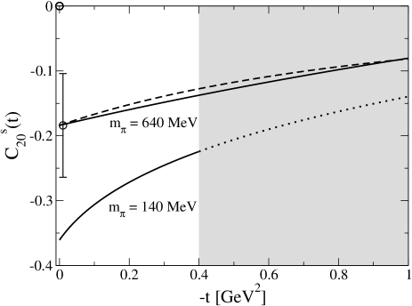
Figure 8: A first glance at the momentum dependence of the form factor $C_{2,0}^{s}(t)$. The quasi-linear $t-$dependence at the pion-mass $m_{\pi}=640$ MeV (solid line) has been normalized to the dipole parametrization of the QCDSF data of ref.[22] (dashed line). The resulting non-linear $t$-dependence in this form factor for smaller values of $m_{\pi}$ is then due to the coupling of the tensor field to the pion cloud, providing an interesting mechanism to obtain “large” negative values at $t=0,\,m_{\pi}=140$ MeV.

6 Summary

The pertinent results of this analysis can be summarized as follows:

1. We have constructed the effective chiral Lagrangean for symmetric, traceless tensor fields of positive parity up to ${\cal O}(p^{2})$ in the covariant framework of Baryon Chiral Perturbation Theory for 2 light quark flavours.

2. Within this covariant framework we have calculated the generalized isovector and isoscalar form factors of the nucleon $A_{2,0}^{v,s}(t,m_{\pi}^{2}),\,B_{2,0}^{v,s}(t,m_{\pi}^{2}),\,C_{2,0}^{v,s}(t,m_{\pi}^{2})$ up to ${\cal O}(p^{2})$, which corresponds to leading-one-loop order. We can exactly reproduce the corresponding non-relativistic ${\cal O}(p^{2})$ results previously obtained in Heavy Baryon ChPT by taking the limit $1/(16\pi^{2}F_{\pi}^{2}M_{0})\rightarrow 0$. Several HBChPT results published recently could not (yet) be reproduced, as they correspond to partial, non-relativistic results from the higher orders ${\cal O}(p^{3},p^{4},p^{5})$.

3. According to our numerical analysis of the quark-mass dependence of the generalized form factors, we have noted that for $B_{2,0}^{s,v}(t)$ and $C_{2,0}^{s,v}(t)$ the observable quark-mass dependencies could be dominated by the (well-known) quark-mass dependence of the mass of the nucleon $M_{N}(m_{\pi}^{2})$. This mass function appears in several places in the chiral results due to kinematical factors in the matrix-element used in the definition of the generalized form factors. Such a “trivial” but numerically significant effect is already known from the analysis of lattice QCD data for the Pauli form factors of the nucleon.

4. The pion-cloud contributions to all three generalized isovector form factors at finite values of $t$ are very small. The momentum dependence of these structures seems to be dominated by (presently) unknown short distance contributions. The situation in this isovector channel reminds us of an analogous role played by chiral dynamics in the isoscalar Dirac and Pauli form factors of the nucleon. At this point we were therefore not able to give predictions for the numerical size of the radii or slopes of these interesting nucleon structure quantities. It is hoped that a global fit to new lattice QCD data at small pion masses and small values of $t$—extrapolated to the physical point with the help of the formulae presented in this work—will lead to first insights into this new field of baryon structure physics [39].

5. The BChPT leading-one-loop results for the generalized isoscalar form factors $A_{2,0}^{s}(t),\,B_{2,0}^{s}(t)$ are quite surprising. As far as the topology of possible Feynman diagrams is concerned, one is reminded of the isovector Dirac and Pauli form factors of the nucleon. A power-counting analysis, however, told us that those diagrams (e.g see Fig.2) from which one would expect large non-analytic contributions in the quark-mass only start to contribute at next-to-leading one-loop order. Our analysis therefore suggests that the momentum-dependence at low values of $t$ is dominated by short-distance physics. A new quality of lattice QCD data for low pion masses and low values of $t$ to constrain some of the unknown couplings is urgently needed before further conclusions can be drawn [39].

6. It is the value of $\langle x\rangle_{\pi}$ of a pion in the chiral limit that controls the magnitude of those long-distance pion-cloud effects in the generalized isoscalar form factors of the nucleon, pointing to the need of a simultaneous analysis of pion and nucleon structure on the lattice and in ChEFT.

7. In the forward limit, the isovector form factor $A_{2,0}^{v}(t\rightarrow 0)$ reduces to $\langle x\rangle_{u-d}$. Our covariant ${\cal O}(p^{2})$ BChPT result for this isovector moment provides a smooth chiral extrapolation function between the high values at large quark-masses from the LHPC collaboration and the lower value known from phenomenology. The required (chiral) curvature according to this new analysis does not originate from the chiral logarithm of the leading-non-analytic quark-mass dependence of this moment—as had been speculated in the literature for the past few years—but is due to an infinite tower of terms $(m_{\pi}/M_{0})^{n}$ with well-constrained coefficients (see Eq.(28)). The well-known leading-one-loop HBChPT result for $\langle x\rangle_{u-d}$ of Eq.(30) was found to be applicable only for chiral extrapolations from the chiral limit to values slightly above the physical pion mass, as expected.

8. Judging from the available (quenched) lattice data of the QCDSF collaboration our ${\cal O}(p^{2})$ BChPT result of Eq.(44) for $A_{2,0}^{s}(t=0)\equiv\langle x\rangle_{u+d}$ also provides a very stable chiral extrapolation function out to quite large values of effective pion masses.

9. A study of the forward limit in the isoscalar sector has led to a first estimate of the contribution of the $u-$ and $d-$quarks to the total spin of a nucleon $J_{u+d}\approx 0.24$. This low value compared to previous determinations arises from the possibility of a small negative contribution of $B_{2,0}^{s}(t=0)\approx-0.06$ at the physical point, driven by pion cloud effects. However, at the moment the uncertainty in such a determination is rather large, due to the poor situation of available data from lattice QCD.

10. In a first glance at the third generalized isoscalar form factor $C_{2,0}^{s}(t)$ the quark-mass dependence was found to be qualitatively different from $A_{2,0}^{s}(t),\,B_{2,0}^{s}(t)$. Its slope contains a chiral singularity $\sim m_{\pi}^{-1}$ and the influence of short distance contributions is suppressed. A first numerical estimate of its slope gives $\rho_{C}^{s}\approx-0.75$ GeV², which is much smaller than the slopes of corresponding Dirac or Pauli form factors. At low t we have also observed significant changes in the momentum dependence of this form factor as a function of the quark-mass, resulting in the estimate $C_{2,0}^{s}(t=0)\approx-0.35$ at the physical point.

11. Throughout this work we have indicated how to estimate possible corrections of higher orders to our leading-one-loop BChPT results. The associated theoretical uncertainties of our ${\cal O}(p^{2})$ calculation have been discussed in detail. Ultimately, in order to judge the stability of our results it is mandatory that we analyse the complete next-to-leading one-loop order. Work in this direction has already started [32].

Finally, we note that the tensor Lagrangeans constructed in section 3 invite a host of further studies, pertaining both to generalized axial form factors of the nucleon [29] and to the energy-momentum-tensor of the nucleon [34].

Appendix A Basic Integrals

The integrals required for one-loop calculations in BChPT can be reduced to two basis integrals in d-dimensions:

$$\Delta_{\pi}\left(m\right) \equiv \frac{1}{i}\int\frac{d^{d}l}{(2\pi)^{d}}\;\frac{1}{m^{2}-l^{2}-i\epsilon},$$ (A.1)

$$H_{11}\left(M^{2},m^{2},p^{2}\right) \equiv \frac{1}{i}\int\frac{d^{d}l}{(2\pi)^{d}}\;\frac{1}{\left(m^{2}-l^{2}-i\epsilon\right)\left(M^{2}-(l-p)^{2}-i\epsilon\right)},$$ (A.2)

where $m\;(M)$ is a mass function involving the mass of the Goldstone Boson (of the Baryon) and $p^{\mu}$ denotes a four-momentum determined by the kinematics.The propagators are shifted into the complex energy-plane by a small amount $\epsilon$ to ensure causality. Utilizing the $\overline{MS}$-renormalization scheme of ref.[4] with

$$L=\frac{\lambda^{d-4}}{16\pi^{2}}\left[\frac{1}{d-4}+\frac{1}{2}\left(\gamma_{E}-1-\ln 4\pi\right)\right],$$ (A.3)

one obtains the dimensionally-regularized results [4]

$$\Delta_{\pi} = 2m^{2}\bigg{(}L+\frac{1}{16\pi^{2}}\ln\frac{m}{\lambda}\bigg{)}+\mathcal{O}(d-4),$$ (A.4)

$$H_{11}(M^{2},m^{2},p^{2}) = -2L-\frac{1}{16\pi^{2}}\bigg{[}-1+\log\frac{M^{2}}{\lambda^{2}}+\frac{p^{2}-M^{2}+m^{2}}{p^{2}}\log\frac{m}{M}$$ (A.5)

$$+\frac{2mM}{p^{2}}\sqrt{1-\bigg{(}\frac{p^{2}-M^{2}-m^{2}}{2mM}\bigg{)}^{2}}\arccos\bigg{(}\frac{m^{2}+M^{2}-p^{2}}{2mM}\bigg{)}\bigg{]}$$

$$+\mathcal{O}(d-4).$$

More complicated integral expressions needed during the calculation are defined via

$$\frac{1}{i}\int\frac{d^{d}l}{(2\pi)^{d}}\,\frac{\{l^{\mu},l^{\mu}l^{\nu}\}}{(m^{2}-l^{2}-i\epsilon)(M^{2}-(l-p)^{2}-i\epsilon)}= \{p^{\mu}H_{11}^{(1)},g^{\mu\nu}H_{11}^{(2)}+p^{\mu}p^{\nu}H_{11}^{(3)}\},$$ (A.6)

$$\frac{1}{i}\int\frac{d^{d}l}{(2\pi)^{d}}\,\frac{l^{\mu}l^{\nu}l^{\alpha}}{(m^{2}-l^{2}-i\epsilon)(M^{2}-(l-p)^{2}-i\epsilon)}= \>(p^{\mu}g^{\mu\alpha}+p^{\nu}g^{\mu\alpha}+p^{\alpha}g^{\mu\nu})\,H_{11}^{(4)}+p^{\mu}p^{\nu}p^{\alpha}\,H_{11}^{(5)}\;.$$ (A.7)

The integrals $H_{11}^{(i)}$ are related to the two basis integrals of Eqs.(A.1-A.2) via well-known tensor-identities [4, 18]. Finally, we note that the integrals involving more than one baryon propagator can be related to the ones defined above via

$$H_{11}^{(i)\prime}(M^{2},m^{2},p^{2})\equiv\frac{\partial}{\partial M^{2}}H_{11}^{(i)}(M^{2},m^{2},p^{2}).$$ (A.8)

Appendix B Regulator Functions

The basis regulator function is defined as [17, 18]

$$R_{11}\left(M^{2},m^{2},p^{2}\right) \equiv \int_{x=1}^{\infty}\!dx\!\int\!\frac{d^{d}l}{(2\pi)^{d}}\left[xM^{2}+(x^{2}-x)p^{2}+(1-x)m^{2}-l^{2}\right]^{-2}.$$ (B.1)

More complicated regulator functions $R_{11}^{(i)},\,i=1\ldots 5$ can be defined in analogy to Eqs.(A.6,A.7). We note that for our ${\cal O}(p^{2})$ calculation of the moments of the GPDs we only need to know these functions up to the power of $m_{\pi}^{2},\,t$ in order to obtain a properly renormalized, scale-independent result, which at the same time is also consistent with the requirements of power-counting. The regulator functions needed for our ${\cal O}(p^{2})$ BChPT calculation (see Appendix C) read

$$R_{11}(M_{0}^{2},m_{\pi}^{2},p^{2}) = \left(2-\frac{m_{\pi}^{2}}{M_{0}^{2}}\right)L+\frac{1}{16\pi^{2}}\Bigg{[}2\log{\frac{M_{0}}{\lambda}}-1-\frac{1}{2}\frac{m_{\pi}^{2}}{M_{0}^{2}}\left(2\log{\frac{M_{0}}{\lambda}}+3\right)\Bigg{]}+...,$$ (B.2)

$$R_{11}^{(1)}(M_{0}^{2},m_{\pi}^{2},p^{2}) = \left(1+\frac{m_{\pi}^{2}}{M_{0}^{2}}\right)L+\frac{1}{16\pi^{2}}\Bigg{[}\log{\frac{M_{0}}{\lambda}}+\frac{1}{2}\frac{m_{\pi}^{2}}{M_{0}^{2}}\left(2\log{\frac{M_{0}}{\lambda}}-1\right)\Bigg{]}+...,$$ (B.3)

$$R_{11}^{(2)}(M_{0}^{2},m_{\pi}^{2},p^{2}) = \left(\frac{1}{3}M_{0}^{2}+\frac{1}{2}m_{\pi}^{2}\right)L+\frac{1}{48\pi^{2}}\Bigg{[}\frac{M_{0}^{2}}{3}\left(3\log{\frac{M_{0}}{\lambda}}-1\right)+\frac{3}{2}m_{\pi}^{2}\left(\log{\frac{M_{0}}{\lambda}}-1\right)\Bigg{]}$$ (B.4)

$$+...,$$

$$R_{11}^{(3)}(M_{0}^{2},m_{\pi}^{2},p^{2}) = \frac{2}{3}L+\frac{1}{48\pi^{2}}\Bigg{[}2\log{\frac{M_{0}}{\lambda}}+\frac{1}{3}+\frac{3}{2}\frac{m_{\pi}^{2}}{M_{0}^{2}}\Bigg{]}+...,$$ (B.5)

The derivatives of the regulator functions needed for the calculation (see Appendix C) read

$${R_{11}^{(2)}}^{\prime}(\tilde{M}^{2},m_{\pi}^{2},\tilde{p}^{2}) = \frac{1}{2}\left(1+\frac{m_{\pi}^{2}}{M_{0}^{2}}\right)L+\frac{1}{32\pi^{2}}\Bigg{[}\log{\frac{M_{0}}{\lambda}}+\frac{m_{\pi}^{2}}{2M_{0}^{2}}\left(2\log{\frac{M_{0}}{\lambda}}-1\right)\Bigg{]}-\frac{t}{384\pi^{2}M_{0}^{2}}$$ (B.6)

$$+...,$$

$${R_{11}^{(3)}}^{\prime}(\tilde{M}^{2},m_{\pi}^{2},\tilde{p}^{2}) = -\frac{m_{\pi}^{2}}{M_{0}^{4}}L+\frac{1}{16\pi^{2}M_{0}^{2}}\Bigg{[}\frac{1}{2}+\frac{m_{\pi}^{2}}{M_{0}^{2}}\left(-\log{\frac{M_{0}}{\lambda}}+1\right)\Bigg{]}+\frac{t}{192\pi^{2}M_{0}^{4}}+...,$$ (B.7)

$${R_{11}^{(4)}}^{\prime}(\tilde{M}^{2},m_{\pi}^{2},\tilde{p}^{2}) = \frac{1}{3}L+\frac{1}{16\pi^{2}}\Bigg{[}\frac{1}{3}\log{\frac{M_{0}}{\lambda}}+\frac{1}{18}+\frac{m_{\pi}^{2}}{4M_{0}^{2}}\Bigg{]}-\frac{t}{576\pi^{2}M_{0}^{2}}+...,$$ (B.8)

$${R_{11}^{(5)}}^{\prime}(\tilde{M}^{2},m_{\pi}^{2},\tilde{p}^{2}) = \frac{1}{16\pi^{2}M_{0}^{2}}\Bigg{[}\frac{1}{3}-\frac{m_{\pi}^{2}}{2M_{0}^{2}}\Bigg{]}+\frac{t}{288\pi^{2}M_{0}^{4}}+...$$ (B.9)

One can clearly observe that all contributions are polynomial in $m_{\pi}^{2}$ (and therefore polynomial in the quark-mass [17]) or polynomial in $t$ [18], as expected. Their addition to the $\overline{MS}$-results therefore just amounts to a shift in the coupling constants [17, 18] of the effective field theory and does not affect the non-analytic quark-mass dependencies, which are the scheme-independent signatures of chiral dynamics.

Appendix C Isovector Amplitudes in ${\cal O}(p^{2})$ BChPT

The five ${\cal O}(p^{2})$ amplitudes in the isovector channel corresponding to the five diagrams of Fig.1 written in terms of the basic integrals

$$I_{11}^{(i)}\left(M^{2},m^{2},p^{2}\right)=H_{11}^{(i)}\left(M^{2},m^{2},p^{2}\right)+R_{11}^{(i)}\left(M^{2},m^{2},p^{2}\right)\;,\quad i=0\ldots 5,$$ (C.1)

of Appendices A and B read

$$Amp^{a+b}= -i\>\frac{\Delta a_{2,0}^{v}\>\>g_{A}}{F_{\pi}^{2}}\>\>\eta^{\dagger}\frac{\tau^{a}}{2}\eta\>\>\overline{u}(p^{\prime})\>\gamma_{\{\mu}\overline{p}_{\nu\}}\>u(p)\>\bigg{[}2m_{\pi}^{2}I_{11}(M_{0}^{2},m_{\pi}^{2},p^{2})$$ (C.2)

$$-m_{\pi}^{2}I_{11}^{(1)}(M_{0}^{2},m_{\pi}^{2},p^{2})+2I_{11}^{(2)}(M_{0}^{2},m_{\pi}^{2},p^{2})\,\bigg{]},$$

$$Amp^{c}= \,i\>\frac{a_{2,0}^{v}g_{A}^{2}}{4F_{\pi}^{2}}\>\>\eta^{\dagger}\frac{\tau^{a}}{2}\eta\>\>\overline{u}(p^{\prime})\>\int^{\frac{1}{2}}_{-\frac{1}{2}}\,du\>\>$$ (C.3)

$$\Bigg{\{}\>\gamma_{\{\mu}\overline{p}_{\nu\}}\>\Bigg{[}-\Delta_{\pi}+4M_{0}^{2}\bigg{(}I_{11}^{(1)}(M_{0}^{2},m_{\pi}^{2},p^{2})-I_{11}^{(3)}(M_{0}^{2},m_{\pi}^{2},p^{2})$$

$$+(2M_{0}^{2}-\tilde{M}^{2})\left(I_{11}^{(3)\prime}(\tilde{M}^{2},m_{\pi}^{2},\tilde{p}^{2})-I_{11}^{(5)\prime}(\tilde{M}^{2},m_{\pi}^{2},\tilde{p}^{2})\right)$$

$$+(d-2)\left(I_{11}^{(4)\prime}(\tilde{M}^{2},m_{\pi}^{2},\tilde{p}^{2})-I_{11}^{(2)\prime}(\tilde{M}^{2},m_{\pi}^{2},\tilde{p}^{2})\right)\bigg{)}\Bigg{]}$$

$$+\,i\,\Delta^{\alpha}\sigma_{\alpha\{\mu}\overline{p}_{\nu\}}\>4M_{0}^{3}\bigg{(}I_{11}^{(3)\prime}(\tilde{M}^{2},m_{\pi}^{2},\tilde{p}^{2})-I_{11}^{(5)\prime}(\tilde{M}^{2},m_{\pi}^{2},\tilde{p}^{2})\bigg{)}$$

$$-\Delta_{\{\mu}\Delta_{\nu\}}\bigg{(}8M_{0}^{3}\,u^{2}\,I_{11}^{(5)\prime}(\tilde{M}^{2},m_{\pi}^{2},\tilde{p}^{2})\bigg{)}\Bigg{\}}\>u(p),$$

$$Amp^{d}= -\,i\>\frac{a_{2,0}^{v}}{F_{\pi}^{2}}\>\>\eta^{\dagger}\frac{\tau^{a}}{2}\eta\>\>\overline{u}(p^{\prime})\>\gamma_{\{\mu}\overline{p}_{\nu\}}\>u(p)\>\Delta_{\pi},$$ (C.4)

$$Amp^{e}= i\>a_{2,0}^{v}\>\>\eta^{\dagger}\frac{\tau^{a}}{2}\eta\>\>\overline{u}(p^{\prime})\>\gamma_{\{\mu}\overline{p}_{\nu\}}\>u(p)\>\mathcal{Z_{N}}.$$ (C.5)

Note that the various couplings and parameters are defined in section 3. $\eta$ denotes the isospin doublet of proton and neutron. The variables in the integral functions are given as

$$\tilde{p}^{2}\,\,=\,\,\tilde{M}^{2} \equiv M_{0}^{2}+\left(u^{2}-\frac{1}{4}\right)t,$$ (C.6)

where $t=\Delta^{2}$ corresponds to the momentum transfer by the tensor fields.

$\mathcal{Z_{N}}$ denotes the Z-factor of the nucleon, calculated to the required ${\cal O}(p^{3})$ accuracy in BChPT. It is obtained from the self-energy $\Sigma_{N}$ at this order via the prescription

$$\mathcal{Z_{N}}=1+\frac{\partial\Sigma_{N}}{\partial\not{p}}\bigg{|}_{\not{p}=M_{0}}+{\cal O}(p^{4}),$$ (C.7)

with

$$\Sigma_{N}=\frac{3g_{A}^{2}}{4F_{\pi}^{2}}(M_{0}+\not{p})\big{[}m_{\pi}^{2}I_{11}(M_{0}^{2},m_{\pi}^{2},p^{2})+(M_{0}-\not{p})\not{p}I_{11}^{(1)}(M_{0}^{2},m_{\pi}^{2},p^{2})-\Delta_{N}\big{]}+{\cal O}(p^{4}).$$ (C.8)

Appendix D BChPT Results in the Isoscalar Channel

D.1 Isoscalar Amplitudes in ${\cal O}(p^{2})$ BChPT

To ${\cal O}(p^{2})$ in BChPT the results in the isoscalar channel are quite simple. The amplitudes corresponding to the Feynman diagrams of Fig.1 can be be simply expressed in terms of results already obtained in the isovector channel discussed in the previous section C. They read

$$\overline{Amp}_{a+b} = 0+{\cal O}(p^{3}),$$ (D.1)

$$\overline{Amp}_{c} = -3\,\frac{a_{2,0}^{s}\eta^{\dagger}{\bf 1}\eta}{a_{2,0}^{v}\eta^{\dagger}\tau^{a}\eta}\,Amp^{c}+{\cal O}(p^{3}),$$ (D.2)

$$\overline{Amp}_{d} = 0+{\cal O}(p^{3}),$$ (D.3)

$$\overline{Amp}_{e} = \frac{a_{2,0}^{s}\eta^{\dagger}{\bf 1}\eta}{a_{2,0}^{v}\eta^{\dagger}\tau^{a}\eta}\,Amp^{e}+{\cal O}(p^{3}).$$ (D.4)

Note that the various couplings and parameters are defined in section 3.

D.2 Estimate of ${\cal O}(p^{3})$ contributions

The contributions from the (higher order) Feynman diagram shown in figure 2 to the generalized isoscalar form factors read

$$\Delta A^{s}_{h.o.}(t,m_{\pi}) = \frac{g_{A}^{2}x_{\pi}^{0}}{32\pi^{2}F_{\pi^{2}}}\int_{-\frac{1}{2}}^{\frac{1}{2}}\!\frac{du}{\tilde{p}^{8}}\,\Bigg{\{}2\tilde{p}^{8}\left(3m_{\pi}^{2}+M_{0}^{2}\right)-t\tilde{p}^{8}+4M_{0}^{2}\left(2M_{0}^{2}+\tilde{m}^{2}\right)\tilde{p}^{6}$$

$$-2M_{0}^{2}\left(11M_{0}^{4}-7\tilde{m}^{2}M_{0}^{2}+2\tilde{m}^{4}\right)\tilde{p}^{4}+12M_{0}^{4}\left(M_{0}^{2}-\tilde{m}^{2}\right)^{2}\tilde{p}^{2}$$

$$+2M_{0}^{2}\bigg{[}-\tilde{p}^{8}+3\tilde{p}^{4}\left(3M_{0}^{4}-\tilde{m}^{4}\right)-2\tilde{p}^{2}\left(M_{0}^{2}-\tilde{m}^{2}\right)\left(7M_{0}^{4}-2\tilde{m}^{2}M_{0}^{2}+\tilde{m}^{4}\right)$$

$$+6M_{0}^{2}\left(M_{0}^{2}-\tilde{m}^{2}\right)^{3}\bigg{]}\log{\frac{\tilde{m}}{M_{0}}}+\frac{2M_{0}^{2}}{\sqrt{2M_{0}^{2}\left(\tilde{p}^{2}+\tilde{m}^{2}\right)-\left(\tilde{p}^{2}-\tilde{m}^{2}\right)^{2}-M_{0}^{4}}}$$

$$\bigg{[}6M_{0}^{10}-4M_{0}^{8}\left(6\tilde{m}^{2}+5\tilde{p}^{2}\right)+M_{0}^{6}\left(36\tilde{m}^{4}+38\tilde{m}^{2}\tilde{p}^{2}+23\tilde{p}^{4}\right)$$

$$-M_{0}^{4}\left(24\tilde{m}^{6}+18\tilde{p}^{2}\tilde{m}^{4}+11\tilde{p}^{4}\tilde{m}^{2}+9\tilde{p}^{6}\right)+M_{0}^{2}\left(6\tilde{m}^{8}+2\tilde{p}^{2}\tilde{m}^{6}\right.$$

$$\left.-5\tilde{p}^{4}\tilde{m}^{4}-2\tilde{p}^{6}\tilde{m}^{2}-\tilde{p}^{8}\right)+\tilde{p}^{2}\left(\tilde{p}^{2}-\tilde{m}^{2}\right)^{3}\left(\tilde{p}^{2}+2\tilde{m}^{2}\right)\bigg{]}\arccos{\left(\frac{M_{0}^{2}+\tilde{m}^{2}-\tilde{p}^{2}}{2M_{0}\tilde{m}}\right)}\Bigg{\}},$$

$$\Delta B^{s}_{h.o.}(t,m_{\pi}) = \frac{g_{A}^{2}x_{\pi}^{0}}{96\pi^{2}F_{\pi}^{2}}\,\frac{M_{N}(m_{\pi})}{M_{0}}\,\int_{-\frac{1}{2}}^{\frac{1}{2}}\!du\,\Bigg{\{}-6M_{0}^{2}+18m_{\pi}^{2}\left(2\log{\frac{M_{0}}{\lambda}}-3\right)+t\left(11-6\log{\frac{M_{0}}{\lambda}}\right)$$ (D.6)

$$-\frac{36M_{0}^{4}}{\tilde{p}^{8}\sqrt{2\left(\tilde{m}^{2}+\tilde{p}^{2}\right)M_{0}^{2}-\left(\tilde{p}^{2}-\tilde{m}^{2}\right)^{2}-M_{0}^{4}}}\bigg{[}M_{0}^{8}-\left(4\tilde{m}^{2}+3\tilde{p}^{2}\right)M_{0}^{6}$$

$$+\left(6\tilde{m}^{4}+5\tilde{p}^{2}\tilde{m}^{2}+3\tilde{p}^{4}\right)M_{0}^{4}-\left(4\tilde{m}^{6}+\tilde{p}^{2}\tilde{m}^{4}+\tilde{p}^{4}\tilde{m}^{2}+\tilde{p}^{6}\right)M_{0}^{2}$$

$$+\tilde{m}^{8}-\tilde{m}^{6}\tilde{p}^{2}\bigg{]}\arccos{\left(\frac{M_{0}^{2}+\tilde{m}^{2}-\tilde{p}^{2}}{2M_{0}\tilde{m}}\right)}-\frac{6M_{0}^{4}}{\tilde{p}^{8}}\bigg{[}2\tilde{p}^{6}-3\left(3M_{0}^{2}-\tilde{m}^{2}\right)\tilde{p}^{4}$$

$$+6\left(M_{0}^{2}-\tilde{m}^{2}\right)^{2}\tilde{p}^{2}+6\left(M_{0}^{2}\tilde{p}^{4}-2M_{0}^{2}\left(M_{0}^{2}-\tilde{m}^{2}\right)\tilde{p}^{2}+\left(M_{0}^{2}-\tilde{m}^{2}\right)^{3}\right)\log{\frac{\tilde{m}}{M_{0}}}\bigg{]}\Bigg{\}},$$

$$+B_{33}^{r}(\lambda)\,\frac{M_{N}(m_{\pi})}{M_{0}}\,\frac{4m_{\pi}^{2}}{\Lambda_{\chi}^{2}}+B_{34}^{r}(\lambda)\,\frac{M_{N}(m_{\pi})}{M_{0}}\,\frac{t}{\Lambda_{\chi}^{2}},$$

$$\Delta C^{s}_{h.o.}(t,m_{\pi}) = \frac{g_{A}^{2}x_{\pi}^{0}M_{0}^{2}}{96\pi^{2}F_{\pi}^{2}}\,\frac{M_{N}(m_{\pi})}{M_{0}}\,\int_{-\frac{1}{2}}^{\frac{1}{2}}\!\frac{du}{\tilde{p}^{8}}\,\Bigg{\{}5\tilde{p}^{8}-9M_{0}^{2}\tilde{p}^{6}-6u^{2}\tilde{p}^{2}\bigg{[}3\tilde{p}^{6}-2M_{0}^{2}\tilde{p}^{4}$$

$$-3M_{0}^{2}\left(M_{0}^{2}-3\tilde{m}^{2}\right)\tilde{p}^{2}-6\left(M_{0}^{3}-M_{0}\tilde{m}^{2}\right)^{2}\bigg{]}-9\left(4u^{2}-1\right)\tilde{p}^{8}\log{\frac{\tilde{m}}{M_{0}}}$$

$$+9M_{0}^{2}\bigg{[}4u^{2}\left(-\tilde{m}^{2}\tilde{p}^{4}+2\tilde{m}^{2}\tilde{p}^{2}\left(\tilde{m}^{2}-M_{0}^{2}\right)+\left(M_{0}^{2}-\tilde{m}^{2}\right)^{3}\right)$$

$$-\tilde{p}^{4}\left(M_{0}^{2}-\tilde{m}^{2}\right)\bigg{]}\log{\frac{\tilde{m}}{M_{0}}}+\frac{9M_{0}^{2}}{\sqrt{2M_{0}^{2}\left(\tilde{m}^{2}+\tilde{p}^{2}\right)-\left(\tilde{p}^{2}-\tilde{m}^{2}\right)^{2}-M_{0}^{4}}}\bigg{[}4u^{2}M_{0}^{8}$$

$$-4\left(4\tilde{m}^{2}+\tilde{p}^{2}\right)u^{2}M_{0}^{6}-\left(-24u^{2}\tilde{m}^{4}+4u^{2}\tilde{p}^{2}\tilde{m}^{2}+\tilde{p}^{4}\right)M_{0}^{4}$$

$$+\left(-16u^{2}\tilde{m}^{6}+20u^{2}\tilde{p}^{2}\tilde{m}^{4}+2\left(1-2u^{2}\right)\tilde{m}^{2}\tilde{p}^{4}+\tilde{p}^{6}\right)M_{0}^{2}$$

$$+\tilde{m}^{2}\left(\tilde{m}^{2}-\tilde{p}^{2}\right)\left(4u^{2}\tilde{m}^{4}-8u^{2}\tilde{m}^{2}\tilde{p}^{2}+\left(4u^{2}-1\right)\tilde{p}^{4}\right)\bigg{]}\arccos{\left(\frac{M_{0}^{2}+\tilde{m}^{2}-\tilde{p}^{2}}{2M_{0}\tilde{m}}\right)}\Bigg{\}},$$

with the new variable

$$\tilde{m}^{2} = m_{\pi}^{2}+\left(u^{2}-\frac{1}{4}\right)t.$$ (D.8)

We note that the contributions of $\Delta A_{2,0}^{s}(t,m_{\pi}),\,\Delta C_{2,0}^{s}(t,m_{\pi})$ are finite at ${\cal O}(p^{3})$ in BChPT, while $\Delta B_{2,0}^{s}(t,m_{\pi})$ contains two new counterterms $B_{33}^{r}(\lambda),\,B_{34}^{r}(\lambda)$ at this order [32].

References

- [1] X. Ji, J. Phys. G24, 1181 (1998) and Ann. Rev. Nucl. Part. Sci. 54, 413 (2003); M. Diehl, Phys. Rep. 388, 41 (2003); A.V. Belitsky and A.V. Radyushkin, Phys. Rep. 418, 1 (2005).
- [2] e.g. see the recent review by V. Bernard and U.-G. Meißner, preprint no. [hep-ph/0611231] and references given therein.
- [3] V. Bernard, H.W. Fearing, T.R. Hemmert and U.-G. Meißner, Nucl. Phys. A635, 121 (1998); [Erratum-ibid. A642 563].
- [4] J. Gasser, M. Sainio, and A. Svarc, Nucl. Phys. B307, 779 (1988).
- [5] B. Kubis and U.-G. Meißner, Nucl. Phys. A679, 698 (2001); M.R. Schindler, J. Gegelia and S. Scherer, Eur. Phys. J. A26, 1 (2005).
- [6] V. Bernard, T.R. Hemmert and U.-G. Meißner, Nucl. Phys. A732, 149 (2004).
- [7] P. Wang, D.B. Leinweber, A.W. Thomas and R.D. Young, preprint no. [hep-ph/0701082].
- [8] T.R. Hemmert and W. Weise, Eur. Phys. J. A15, 487 (2002).
- [9] QCDSF Collaboration (M. Göckeler et al.), Phys. Rev. D71, 034508 (2005).
- [10] C. Alexandrou, G. Koutsou, J.W. Negele and A. Tsapalis, Phys. Rev. D74, 034508 (2006).
- [11] C.F. Perdrisat, V. Punjabi and M. Vanderhaeghen, preprint no. [hep-ph/0612014].
- [12] K. de Jager, preprint no. [nucl-ex/0612026], to appear in the Proceedings of “Workshop on the Shape of Hadrons”, Athens, Greece, 27-29 Apr 2006.
- [13] J.-W. Chen and X. Ji, Phys. Rev. Lett. 88, 052003 (2002).
- [14] A.V. Belitsky and X. Ji, Phys. Lett. B538, 289 (2002).
- [15] S. Ando, J.-W. Chen and C.-W. Kao, Phys. Rev. D74, 094013 (2006).
- [16] M. Diehl, A. Manashov and A. Schäfer, Eur. Phys. J. A29, 315 (2006) and preprint no. [hep-ph/0611101].
- [17] T. Becher and H. Leutwyler, Eur. Phys. J. C9, 643 (1999).
- [18] T.A. Gail and T.R. Hemmert, in Proceedings of ECT* Workshop “Lattice QCD, Chiral Perturbation Theory and Hadron Phenomenology”, Trento, Italy, 2-6 Oct 2006, preprint no. [hep-ph/0611072] and forthcoming work.
- [19] M. Procura, T.R. Hemmert and W. Weise, Phys. Rev. D69, 034505 (2004); QCDSF-UKQCD Collaboration (A. Ali Khan et al.), Nucl. Phys. B689, 175 (2004); V. Bernard, T.R. Hemmert and U.-G. Meißner, Phys. Lett. B622,141 (2005); M. Procura, B.U. Musch, T. Wollenweber, T.R. Hemmert and W. Weise, Phys. Rev. D73, 114510 (2006).
- [20] S. Boffi, B. Pasquini and M. Traini, Nucl. Phys. B649, 243 (2003).
- [21] K. Göke et al., preprint no. [hep-ph/0702031].
- [22] QCDSF Collaboration (M. Göckeler et al.), Phys. Rev. Lett. 92, 042002, (2004) and Nucl. Phys. Proc. Suppl. 128, 203 (2004).
- [23] LHPC-SESAM Collaboration (Ph. Hägler et al.), Phys. Rev. D68, 034505 (2003).
- [24] LHPC Collaboration (R.G. Edwards et al.), preprint no. [hep-lat/0610007], to appear in the Proceedings of “Lattice 2006”, Tucson, Arizona, 23-28 Jul 2006.
- [25] J.A. McGovern and M.C. Birse, Phys. Rev. D74, 097501 (2006).
- [26] see http://www-spires.dur.ac.uk/hepdata/pdf3.html
- [27] J.F. Donoghue and H. Leutwyler, Z. Phys. C52, 343 (1991).
- [28] N. Kivel and M. V. Polyakov, preprint no. [hep-ph/0203264]; M. Diehl, A. Manashov and A. Schäfer, Phys. Lett. B622, 69 (2005).
- [29] M. Dorati and T.R. Hemmert, “Generalized Axial Form Factors of the Nucleon”, in preparation.
- [30] O.V. Teryaev, preprint no. [hep-ph/9904376]; S.J. Brodsky, D.S. Hwang, B.-Q. Ma and I. Schmidt, Nucl. Phys. B593, 311 (2001).
- [31] J. Gasser and H. Leutwyler, Annals Phys. 158, 142 (1984).
- [32] M. Dorati, Ph. Hägler and T.R. Hemmert, “Moments of nucleon GPDs at next-to-leading one-loop order”, in preparation.
- [33] e.g. see chapter 3.1 in V. Bernard, N. Kaiser and U.-G. Meißner, Int. J. Mod. Phys. E4 (1995).
- [34] T.R. Hemmert et al., “The energy-momentum-tensor of a nucleon from the viewpoint of ChPT”, in preparation.
- [35] W. Detmold, W. Melnitchouk, J.W. Negele, D.B. Renner, A.W. Thomas, Phys. Rev. Lett. 87: 172001 (2001); LHCP Collaboration (D. Dolgov et al.), Phys. Rev. D66, 034506 (2002).
- [36] D. Arndt and M.J. Savage, Nucl. Phys. A697, 429 (2002).
- [37] J.-W. Chen and X. Ji, Phys. Lett. B523, 107 (2001).
- [38] T.R. Hemmert, M. Procura and W. Weise, Phys. Rev. D68, 075009 (2003).
- [39] LHPC collaboration, (spokesperson J. Negele), in preparation; QCDSF collaboration, (spokesperson G. Schierholz), in preparation.
- [40] V. Bernard, T.R. Hemmert and U.-G. Meißner, Phys. Lett. B565, 137 (2003); T.R. Hemmert, B.R. Holstein and J. Kambor J. Phys. G24, 1831 (1998).
- [41] M. Dorati, Laurea Thesis, University of Pavia, Pavia, Italy (2005).
- [42] X. Ji, Phys. Rev. Lett. 78, 610 (1997).
- [43] M. Glück, E. Reya and I. Schienbein, Eur. Phys. J. C10, 313 (2000).
- [44] P. Mergell, U.-G. Meißner and D. Drechsel, Nucl. Phys. A596, 367 (1996).
- [45] LHPC-SESAM Collaboration (Ph. Hägler et al.), Phys. Rev. Lett. 93, 112001 (2004).
- [46] D. Binosi and L. Theussl, Comput. Phys. Commun. 161, 76 (2004).