Nuclear reaction studies of unstable nuclei using relativistic mean field formalisms in conjunction with Glauber model

Abstract

We study nuclear reaction cross-sections for stable and unstable projectiles and targets within Glauber model, using densities obtained from various relativistic mean field formalisms. The calculated cross-sections are compared with the experimental data in some specific cases. We also evaluate the differential scattering cross-sections at several incident energies, and observe that the results found from various densities are similar at smaller scattering angles, whereas a systematic deviation is noticed at large angles. In general, these results agree fairly well with the experimental data.

I Introduction

Study of unstable nuclei with radioactive ion beam (RIB) facilities has opened an exciting channel to look for some crucial issues in context of both nuclear structure and nuclear astrophysics oza01 ; kho04 ; nun05 . Unstable nuclei play an influential, and in some cases dominant, role in many phenomena in the cosmos such as novae, supernovae, X-ray bursts, and other stellar explosions. At extremely high temperatures ($>10^{8}$ K) of these astrophysical environments, the interaction times between nuclei can be so short ($\sim$ seconds) that unstable nuclei formed in a nuclear reaction can undergo subsequent reactions before they decay. Sequences of (predominantly unmeasured) nuclear reactions occurring in exploding stars are therefore quite different than sequences occurring at lower temperatures, for example, characteristic of those occurring in Sun. The direct study of stellar properties in ground-based laboratories has become more attractive, due to the availability of RIBs, for example the study of ¹⁸Ne induced neutron pick-up reaction could reveal information about the exotic ¹⁵O+¹⁹Ne reaction happening in the CNO cycle in burning stars. Study of the structure and reactions of unstable nuclei is therefore required to improve our understanding of the astrophysical origin of atomic nuclei and the evolution of stars and their (sometimes explosive) deaths.

Experimental study of unstable nuclei has considerably advanced through the technique of using secondary radioactive beams. The quantities measured in the study include various inclusive cross-sections, for example, reaction or interaction cross-sections, nucleon-removal cross-sections, Coulomb breakup cross-sections and momentum distributions of a fragment. These quantities have played an important role to reveal the nuclear structure of unstable nuclei, particularly halo structure near the drip line tan96 . The total reaction cross-section ($\sigma_{r}$) is one of the most fundamental quantities characterizing the nuclear reactions and to probe for nuclear structure details. Recent studies using RIB have demonstrated a large enhancement of $\sigma_{r}$ induced by neutron rich nuclei, which has been interpreted as neutron halo tan85 ; kob88 ; han89 ; mit87 (such as ¹¹Li, ^11,14Be, etc.) and neutron skin structure mit87 (such as ⁶He and ⁸He). The halo structure of ¹¹Li seems to be consistent with all the experimental results including the enhancement of interaction cross-section $\sigma_{I}$, the enhancement of two-neutron removal cross-section ($\sigma_{2n}$) and the narrow peak in the momentum distribution of fragmentation of ⁹Li.

At present the Glauber model is a standard tool to calculate the cross-sections because it can account for a significant part of breakup effects which play an important role in the reaction of a weakly bound nucleus var02 ; abu03 . The Glauber model, based on the independent individual nucleon-nucleon collisions in the overlap zone of the colliding nuclei gla59 , has been used extensively to explain the observed nuclear reaction cross-section for various systems at high energies ber89 ; far01 . This model requires the structure information, namely the density profiles, of the nuclei involved. This information has to be provided by nuclear structure models, like the relativistic mean field (RMF) theory which is effectively used for this purpose recently bhagwat ; shukla05 .

The RMF formalism is well suited for the studies of exotic nuclei patra91 . It takes into account the spin orbit interaction automatically, unlike to the non-relativistic case. The parameters are fitted by taking into account the properties of few spherical nuclei. The inclusion of rho-meson takes into account the proton-neutron asymmetry and gives an impression that the theory can be used to nuclei far away from the valley of $\beta$-stability. Apart from these, the advantage of the RMF model is the microscopic calculations of nuclear structure starting from the Lagrangian with same parameters applicable for the whole nuclear chart and beyond. The recent extension of this formalism with field theory motivated effective Lagrangian approach (E-RMF) ser97 ; fur96 could extend the applicability of this model to neutron stars and infinite nuclear matter aru04 . Hence this model provides us better predictability to explore the features of exotic nuclei.

The main objective of the present work is to study the nuclear reaction cross-section using RMF and E-RMF nuclear densities in conjunction with the Glauber model. The paper is presented as follows. In section II, we discuss in brief the formalism used in the present work. In section III, we discuss our results for the ground state properties of few selected light mass nuclei and cross-sections of reactions involving them. The summary and concluding remarks are given in section IV.

II Formalism

II.1 E-RMF approach for nuclear structure

The details of the standard RMF formalism for finite nuclei can be found in Refs. patra91 . The recent extension of RMF formalism based upon the field theory motivated effective Lagrangian approach, known as E-RMF, can be found in Refs. patra01 ; patra01a . The energy density functional of the E-RMF model for finite nuclei ser97 ; fur96 ; patra01 ; patra01a is written as

$$\mathcal{E}(\mathbf{r}) = \sum_{\alpha}\varphi_{\alpha}^{\dagger}\Bigg{\{}-i\mbox{\boldmath$\alpha$}\!\cdot\!\mbox{\boldmath$\nabla$}+\beta(M-\Phi)+W+\frac{1}{2}\tau_{3}R+\frac{1+\tau_{3}}{2}A$$ (1)

$$-\frac{i}{2M}\beta\mbox{\boldmath$\alpha$}\!\cdot\!\left(f_{v}\mbox{\boldmath$\nabla$}W+\frac{1}{2}f_{\rho}\tau_{3}\mbox{\boldmath$\nabla$}R+\lambda\mbox{\boldmath$\nabla$}A\right)+\frac{1}{2M^{2}}\left(\beta_{s}+\beta_{v}\tau_{3}\right)\Delta A\Bigg{\}}\varphi_{\alpha}$$

$$\hbox{}+\left(\frac{1}{2}+\frac{\kappa_{3}}{3!}\frac{\Phi}{M}+\frac{\kappa_{4}}{4!}\frac{\Phi^{2}}{M^{2}}\right)\frac{m_{s}^{2}}{g_{s}^{2}}\Phi^{2}-\frac{\zeta_{0}}{4!}\frac{1}{g_{v}^{2}}W^{4}$$

$$\hbox{}+\frac{1}{2g_{s}^{2}}\left(1+\alpha_{1}\frac{\Phi}{M}\right)\left(\mbox{\boldmath$\nabla$}\Phi\right)^{2}-\frac{1}{2g_{v}^{2}}\left(1+\alpha_{2}\frac{\Phi}{M}\right)\left(\mbox{\boldmath$\nabla$}W\right)^{2}$$

$$\hbox{}-\frac{1}{2}\left(1+\eta_{1}\frac{\Phi}{M}+\frac{\eta_{2}}{2}\frac{\Phi^{2}}{M^{2}}\right)\frac{{m_{v}}^{2}}{{g_{v}}^{2}}W^{2}-\frac{1}{2g_{\rho}^{2}}\left(\mbox{\boldmath$\nabla$}R\right)^{2}-\frac{1}{2}\left(1+\eta_{\rho}\frac{\Phi}{M}\right)\frac{m_{\rho}^{2}}{g_{\rho}^{2}}R^{2}$$

$$\hbox{}-\frac{1}{2e^{2}}\left(\mbox{\boldmath$\nabla$}A\right)^{2}+\frac{1}{3g_{\gamma}g_{v}}A\Delta W+\frac{1}{g_{\gamma}g_{\rho}}A\Delta R,$$

where the index $\alpha$ runs over all occupied states $\varphi_{\alpha}(\mathbf{r})$ of the positive energy spectrum, $\Phi\equiv g_{s}\phi_{0}(\mathbf{r})$, $W\equiv g_{v}V_{0}(\mathbf{r})$, $R\equiv g_{\rho}b_{0}(\mathbf{r})$ and $A\equiv eA_{0}(\mathbf{r})$.

The terms with $g_{\gamma}$, $\lambda$, $\beta_{s}$ and $\beta_{v}$ take care of effects related with the electromagnetic structure of the pion and the nucleon (see Ref. fur96 ). Specifically, the constant $g_{\gamma}$ concerns the coupling of the photon to the pions and the nucleons through the exchange of neutral vector mesons. The experimental value is $g_{\gamma}^{2}/4\pi=2.0$. The constant $\lambda$ is needed to reproduce the magnetic moments of the nucleons. It is defined by

$$\lambda=\frac{1}{2}\lambda_{p}(1+\tau_{3})+\frac{1}{2}\lambda_{n}(1-\tau_{3}),$$ (2)

with $\lambda_{p}=1.793$ and $\lambda_{n}=-1.913$ the anomalous magnetic moments of the proton and the neutron, respectively. The terms with $\beta_{s}$ and $\beta_{v}$ contribute to the charge radii of the nucleon fur96 .

The energy density contains tensor couplings and scalar-vector and vector-vector meson interactions in addition to the standard scalar self interactions $\kappa_{3}$ and $\kappa_{4}$. The E-RMF formalism can be interpreted as a covariant formulation of density functional theory as it contains all the higher order terms in the Lagrangian by expanding it in powers of the meson fields. The terms in the Lagrangian are kept finite by adjusting the parameters. Further insight into the concepts of the E-RMF model can be obtained from Ref. fur96 . It is worth mentioning that the standard RMF Lagrangian is obtained by ignoring the vector-vector and scalar-vector cross interactions, and does not need any separate discussion. The field equations and numerical details can be obtained in Refs. patra91 ; patra01 ; patra01a . The set of coupled equations is solved numerically by a self-consistent iteration method. The baryon, scalar, isovector, proton and tensor densities are

$$\rho(r) = \sum_{\alpha}\varphi_{\alpha}^{\dagger}(r)\varphi_{\alpha}(r)\,,$$ (3)

$$\rho_{s}(r) = \sum_{\alpha}\varphi_{\alpha}^{\dagger}(r)\beta\varphi_{\alpha}(r)\,,$$ (4)

$$\rho_{3}(r) = \sum_{\alpha}\varphi_{\alpha}^{\dagger}(r)\tau_{3}\varphi_{\alpha}(r)\,,$$ (5)

$$\rho_{\rm p}(r) = \sum_{\alpha}\varphi_{\alpha}^{\dagger}(r)\left(\frac{1+\tau_{3}}{2}\right)\varphi_{\alpha}(r)\,,$$ (6)

$$\rho_{\rm T}(r) = \sum_{\alpha}\frac{i}{M}\mbox{\boldmath$\nabla$}\!\cdot\!\left[\varphi_{\alpha}^{\dagger}(r)\beta\mbox{\boldmath$\alpha$}\varphi_{\alpha}(r)\right]\,,$$ (7)

$$\rho_{\rm T,3}(r) = \sum_{\alpha}\frac{i}{M}\mbox{\boldmath$\nabla$}\!\cdot\!\left[\varphi_{\alpha}^{\dagger}(r)\beta\mbox{\boldmath$\alpha$}\tau_{3}\varphi_{\alpha}(r)\right]\,.$$ (8)

For the calculation of ground state properties of finite nuclei, we refer the readers to Refs. patra91 ; patra01 ; patra01a .

II.2 Glauber model for nuclear reactions

The theoretical formalism to calculate the nuclear reaction cross-section using Glauber approach has been given by R. J. Glauber gla59 . For sake of completeness, here, we briefly outline the steps of derivations following the notation of Ref. gla59 .

The standard Glauber form for the reaction cross-section at high energies, is expressed gla59 as:

$$\sigma_{R}=2\pi\int\limits_{0}^{\infty}b[1-T(b)]db\;,$$ (9)

where $T(b)$, the transparency function, is the probability that at an impact parameter $b$ the projectile pass through the target without interacting. This function $T(b)$ is calculated in the overlap region between the projectile and target where the interactions are assumed to result from single nucleon-nucleon collision and is given by

$$T(b)=\exp\left[-\sum\limits_{i,j}\overline{\sigma}_{ij}\int d\vec{s}\overline{\rho}_{ti}\left(s\right)\overline{\rho}_{pj}\left(\left|\vec{b}-\vec{s}\right|s\right)\right]\;.$$ (10)

Here, the summation indices $i$, $j$ run over proton and neutron and subscript $p$ and $t$ refers to projectile and target respectively. $\overline{\sigma}_{ij}$ is the experimental nucleon-nucleon reaction cross-section which varies with respect to energy. The $z$-integrated densities $\overline{\rho}(\omega)$ are defined as

$$\overline{\rho}(\omega)=\int\limits_{-\infty}^{\infty}\rho\left(\sqrt{\omega^{2}+z^{2}}\right)dz\;,$$ (11)

with $\omega^{2}=x^{2}+y^{2}$. The parameters $\sigma_{NN}$, $\alpha$, and $\beta$ usually depend on either the proton-proton (neutron-neutron) or proton-neutron case, but we have used some appropriate average values in the present calculations kar75 . The argument of $T(b)$ in eq. (10) is $\left|\vec{b}-\vec{s}\right|$, which stands for the impact parameter between $i^{th}$ and $j^{th}$ nucleons.

The Glauber model agrees very well with the experimental data at high energies. However, this model fails to describe, reasonably, the collisions induced at relatively low energies. In such case the present version of Glauber model is modified in order to take care of finite range effects in profile function and Coulomb modified trajectories. Thus for finite range approximations, the transparency function is given by

$$T(b)=\exp\left[-\int\nolimits_{p}\int\nolimits_{t}\sum\limits_{i,j}\left[\Gamma_{ij}\left(\vec{b}-\vec{s}+\vec{t}\right)\right]\overline{\rho}_{pi}\left(\vec{t}\right)\overline{\rho}_{tj}\left(\vec{s}\right)d\vec{s}d\vec{t}\right]\;.$$ (12)

Here the profile function $\Gamma_{ij}$ is given by

$$\Gamma_{ij}(b_{eff})=\frac{1-i\alpha}{2\pi\beta_{NN}^{2}}\sigma_{ij}\exp\left(-\frac{b_{eff}^{2}}{2\beta_{NN}^{2}}\right)\;,$$ (13)

where $b_{eff}=\left|\vec{b}-\vec{s}+\vec{t}\right|$, $\vec{b}$ is the impact parameter and $\vec{s}$ and $\vec{t}$ are just the dummy variables for integration over the $z$-integrated target and projectile densities.

II.2.1 Differential cross-section

The differential elastic cross-section by the ratio to the Rutherford cross-section is given by,

$$\frac{d\sigma}{d\Omega}=\frac{\left|F(q)\right|^{2}}{\left|F_{coul}(q)\right|^{2}}\;.$$ (14)

$F(q)$ and $F_{coul}(q)$ are the elastic and Coulomb (elastic) scattering amplitudes, respectively.

The elastic scattering amplitude $F(q)$ is written as

$$F(q)=e^{i\chi_{s}}\left\{F_{coul}(q)+\frac{iK}{2\pi}\int db\exp[-i{\vec{q}}\cdot{\vec{b}}+2i\eta{\ln(Kb)}]T(b)\right\}$$ (15)

with the Coulomb elastic scattering amplitude $F_{coul}(q)$ given by

$$F_{coul}(q)=\frac{-2\eta K}{q^{2}}\exp\left\{-2i\eta{\ln}\left(\frac{q}{2K}\right)+2i\arg\Gamma\left(1+i\eta\right)\right\}\;.$$ (16)

Here $\eta=Z_{P}Z_{T}e^{2}$/$\hbar v$ is the Sommerfield parameter, $v$ is the incident velocity, and $\chi_{s}=-2\eta\ln(2Ka)$ with $a$ being screening radius gla59 . The elastic differential cross-section does not depend on the screening radius $a$.

III Results and Discussion

III.1 Ground state properties from RMF models

There exist a number of parameter sets for solving the standard RMF as well as E-RMF Lagrangians. In our previous paper shukla05 we have calculated reaction cross-sections with densities obtained from various interactions. In the present work, we employ the SIG-OM set for RMF which has been recently used by Haidari et al. haid07 and G2 patra01 for E-RMF calculations.

III.1.1 Binding Energies

We have presented the calculated binding energy using RMF and E-RMF theories in Table I. The experimental data taken from Ref. audi have also been given for comparison. It is evident from Table II that both the calculated binding energies are similar and slightly overestimate in comparison with experimental binding energies. However, these differences with experimental values are small and may be attributed to the fact that for light mass region of the periodic table, mean field is not saturated. To get a qualitative estimation of the binding energy, the RMF as well as E-RMF results are trust worthy and can be used for further calculations in this region.

Table 1: The ground state properties of the nuclei involved in reaction cross-section study. Experimental binding energies have been taken from audi . The SIG-OM and G2 sets are chosen for RMF and E-RMF parametrizations, respectively.

nuclei	charge radii (in fm)			binding energy (in MeV)
	RMF	E-RMF	Expt. ang04	RMF	E-RMF	Expt. audi
12C	2.466	2.497	2.470	84.061	87.230	92.162
6Li	2.525	2.512	2.539	29.377	31.936	31.994
7Li	2.363	2.354	2.431	33.444	36.538	39.244
8Li	2.281	2.264		38.664	42.214	41.277
9Li	2.234	2.202		44.825	48.761	45.341
10Li	2.261	2.230		47.168	50.937	45.316
11Li	2.291	2.266		50.453	53.997	45.640
7Be	2.685	2.680		31.736	34.862	37.600
8Be	2.497	2.504		39.146	42.706	56.500
9Be	2.401	2.405	2.518	47.805	51.620	58.165
10Be	2.341	2.336		57.328	61.265	64.977
11Be	2.368	2.367		61.911	65.627	65.481
12Be	2.393	2.397		67.341	70.735	68.650
13Be	2.411	2.406		64.982	69.109	68.549
14Be	2.428	2.412		63.097	67.892	69.916
8B	2.769	2.776		34.718	38.359	37.737
9B	2.578	2.598		45.502	49.392	56.314
10B	2.472	2.492	2.428	57.556	61.420	64.751
11B	2.412	2.428	2.406	70.562	74.213	76.205
12B	2.434	2.453		77.411	80.784	79.575
13B	2.456	2.478		85.090	88.027	84.453
14B	2.469	2.479		84.044	87.841	85.422
15B	2.482	2.478		83.490	88.098	88.185
16B	2.495	2.477		83.623	88.795	88.144
17B	2.509	2.476		83.976	89.925	89.522

III.1.2 Nuclear Radii

The root mean square (rms) charge radius ($r_{c}$) is obtained from the point proton rms radius through the relation given below patra91 :

$$r_{c}=\sqrt{r_{p}^{2}+0.64}\;,$$

considering the size of proton radius as 0.8 fm. In Table I, we have presented the calculated nuclear charge radii using RMF and E-RMF models as well as the experimental values, wherever available. We can notice from Table I that both models, RMF as well as E-RMF give similar result for nuclear radii and both account fairly well for the experimentally observed values. Since the charge radius is obtained from the density profile and our RMF and E-RMF results for $r_{c}$ matches excellently with experimental results, we can use these density profiles in the cross-section calculations reliably, which is the main objective of the present study.

III.2 Input for Glauber model

The main input required for calculating the cross-sections using Glauber model includes the target and projectile nuclear densities. The nuclear densities obtained from RMF calculations are then fitted by a sum of Gaussian functions with appropriate coefficients $c_{i}$ and ranges $a_{i}$ chosen for the respective nuclei as,

$$\rho(r)=\sum\limits_{i=1}^{N}c_{i}\exp[-a_{i}r^{2}].$$ (17)

In the present work, the RMF and E-RMF densities have been fitted with a sum of two Gaussians and the calculated coefficients $c_{1},c_{2}$ and ranges $a_{1},a_{2}$ are listed in Table II.

Table 2: The coefficients of Gaussian functions fitted to mimic the density distributions from RMF with SIG-OM and E-RMF with G2 parameter sets. The first line corresponds to SIG-OM and the second line to G2 parametrizations.

Nuclei	c1	a1	c2	a2	Nuclei	c1	a1	c2	a2
12C	-1.19290	0.43150	1.41910	0.36777	8B	-1.05597	0.34652	1.28006	0.33463
	-3.77056	0.37809	3.96943	0.36006		-0.03535	0.75948	0.22188	0.28100
6Li	-1.19320	0.35724	1.42228	0.35709	9B	-0.05555	0.71516	0.27596	0.29664
	-1.20692	0.39464	1.39716	0.38081		-0.14934	0.51161	0.33920	0.30400
7Li	-1.18917	0.31651	1.41291	0.31651	10B	-0.16001	0.56271	0.38264	0.31404
	-0.02297	0.90405	0.20935	0.29855		-1.21376	0.39463	1.40784	0.35375
8Li	-1.18507	0.36369	1.40981	0.34895	11B	-0.32664	0.49989	0.55114	0.33064
	-0.04539	0.70103	0.23248	0.28682		-2.79365	0.38139	2.99014	0.36013
9Li	-0.02607	0.92972	0.24542	0.28133	12B	-0.49301	0.44359	0.69585	0.32118
	-0.07409	0.60134	0.26200	0.27935		-3.12130	0.36071	3.30124	0.34123
10Li	-0.03526	0.79222	0.23711	0.25465	13B	-0.77107	0.40334	0.95417	0.31709
	-0.07966	0.56516	0.25466	0.25458		-3.56218	0.34485	3.72662	0.32706
11Li	-0.05229	0.67219	0.23641	0.23543	14B	-0.38333	0.43538	0.56403	0.27802
	-0.09683	0.51846	0.25806	0.23719		-2.54155	0.33298	2.70540	0.30913
7Be	-1.19498	0.31920	1.41997	0.31896	15B	-0.29069	0.44877	0.46814	0.25388
	-0.01977	0.96010	0.20625	0.29648		-0.99177	0.33718	1.15357	0.28066
8Be	-0.02025	0.98637	0.24419	0.30083	16B	-0.24920	0.45530	0.42450	0.23682
	-0.07016	0.61682	0.25782	0.29849		-0.55398	0.34711	0.71249	0.25353
9Be	-0.06240	0.69377	0.28340	0.30012	17B	-0.22619	0.45154	0.39655	0.22176
	-0.17128	0.49902	0.36183	0.30951		-0.43556	0.34777	0.59030	0.23519
10Be	-0.12156	0.59723	0.34318	0.30291
	-0.40674	0.43037	0.59982	0.32511
11Be	-0.15051	0.54021	0.35239	0.28195
	-0.39959	0.40983	0.57775	0.30105
12Be	-0.19523	0.49296	0.37849	0.26865
	-0.47247	0.38545	0.63604	0.28738
13Be	-0.14949	0.52383	0.33391	0.24652
	-0.25171	0.42035	0.41548	0.25339
14Be	-0.12420	0.54603	0.30791	0.22839
	-0.19132	0.43615	0.353435	0.23129

This fitting makes it possible to obtain analytic expression for the transparency functions as defined in eqs. (10) and (12) and hence simplify further numerical calculations oga92 . We have shown the density distribution plot of ¹¹Li using RMF (spherical coordinate basis-CB) and E-RMF (CB) nuclear densities in Fig. 1(a), to have a comparable look. The results of RMF and E-RMF are quite similar except a small difference at centre. We have repeated the same calculations for ¹²C density using RMF and E-RMF numerical methods and the results are plotted in Fig. 1(b).

Figure 1: Comparison of density distribution obtained from RMF and E-RMF calculations: (a) for ¹¹Li and (b) for ¹²C nucleus.

Table 3: The averaged nucleon-nucleon cross-sections $\sigma_{NN}$ and other parameters used for calculation of profile function.

Energy	30	49	85	100	120	150	200
(in MeV/
nucleon)
$\sigma_{NN}$	19.6	10.4	6.1	5.29	4.72	3.845	3.28
$\alpha_{NN}$	0.87	0.94	1.0	1.435	1.38	1.245	0.93
$\beta_{NN}$	0.0	0.0	0.0	1.02	1.07	1.15	1.24
Energy	325	425	500	625	800	1100	2200
(in MeV/
nucleon)
$\sigma_{NN}$	3.03	3.025	3.62	4.0	4.26	4.32	4.335
$\alpha_{NN}$	0.305	0.36	0.04	-0.095	-0.07	-0.275	-0.335
$\beta_{NN}$	0.62	0.48	0.125	0.16	0.21	0.22	0.26

The calculation of profile function $\Gamma$ requires some phenomenological parameters related to nucleon-nucleon cross-section. These parameters $\sigma_{NN},$ $\alpha,$ and $\beta$ at various energies are taken from Refs. far01 ; kar75 and tabulated in Table III for sake of completness. Here $\sigma_{NN}$ represents the total cross-section of N-N collision, $\alpha_{NN}$ is the ratio of the real to the imaginary part of the forward nucleon-nucleon scattering amplitude and $\beta_{NN}$ is basically the slope parameter which determines the fall-of the angular distribution of the N-N elastic scattering. Though these parameters in general depend on the isospin of the nucleons (pp, nn, pn), appropriate average values are taken by interpolating a given set.

III.3 Total reaction cross-section

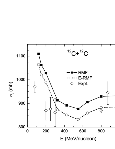
Figure 2: The total reaction cross-section ($\sigma_{r}$) for ¹²C+¹²C system. Experimental data are also shown in the figure with error bars abu03 ; jar78 .

The total reaction cross-sections at different incident energies have been calculated for various systems and compared with the experimental results buen84 , if available. The reaction cross-section with stable and unstable beams using stable target such as ¹²C are within experimental reach and are being studied extensively yan02 . As a first application to nuclear reaction studies, we have calculated the total reaction cross-section for ¹²C+¹²C system and compared with the experimental results abu03 ; jar78 . It can be seen from Fig. 2 that the agreement of $\sigma_{r}$ using E-RMF nuclear densities is excellent for almost all incident energies (energy/nucleon), particularly at higher values. The calculated E-RMF cross-section is slightly off at lower energies which is easily understandable as it is well studied that the Glauber model works better at higher incident energies in comparison to the lower incident energies. This disagreement is due to the significant role played by the repulsive Coulomb potential whose effects are obvious in the low-energy range. Such a Coulomb effect breaks the characteristic Glauber assumption that the projectile travels along straight-line trajectories. However, our results using E-RMF nuclear densities successfully produce the qualitative trend of experimental results. Here it is interesting to see that the calculations using RMF densities also matches reasonably with the experimental values but the results at lower incident energies are quite off.

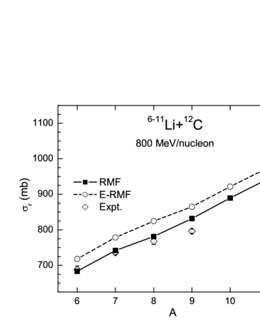
Figure 3: The total reaction cross-section ($\sigma_{r}$) at 800 MeV/nucleon for Li isotopes as projectile and ¹²C as target. Experimental data with error bars oza01 ; tan96 ; tan85 are also shown.

In Figs. 3 and 4, we have shown the comparison of experimental oza01 ; tan96 ; tan85 and calculated $\sigma_{r}$ for ^6-11Li+¹²C, ^7-14Be+¹²C and ^8-17B+¹²C systems at fixed incident energy (800 MeV/nucleon). The trends of the calculations for the different projectiles [Figs. 3 and 4] are basically the same.

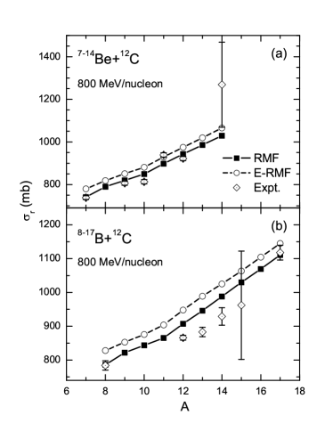
Figure 4: (a) Same as Fig. 3, but for Be isotopes as projectile. (b) Same as Fig. 3, but for B isotopes as projectile. Experimental data are taken from oza01 ; tan96 ; tan85

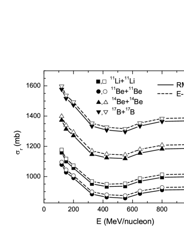
Figure 5: Total reaction cross-section for ¹¹Li+¹¹Li, ¹¹Be+¹¹Be, ¹⁴Be+¹⁴Be and ¹⁷B+¹⁷B with RMF and E-RMF densities as input for various incident energies.

So far we have discussed the reactions involving stable and unstable beams on stable target. To measure the nuclear reaction cross-section with unstable beam and unstable target is one of the major challenges for experimental nuclear physicists. Such measurements would be helpful for the better understanding of many astrophysical phenomena as well as in determining the energy and matter evolution at stellar sites. As more extensive observational data is gathered from earth and space observatories, an ever-greater demand is placed on our knowledge of the basic physical processes that probe astrophysical phenomena. Considerable efforts at Institute of Modern Physics, CAS (China) and at RIKEN (Japan) are underway to look for RIB+RIB cross-section using RIB as internal target with RIB projectile. Although such measurements are not feasible with presently available experimental techniques, yet the fast advancement in RIB techniques may provide us this facility in next few years or so. Such experiments will be decisive in getting precise information about the structure of halo nuclei. In this view, we have presented the calculated $\sigma_{r}$ for few RIB+RIB systems, namely for ¹¹Li+¹¹Li, ¹¹Be+¹¹Be, ¹⁴Be+¹⁴Be and ¹⁷B+¹⁷B in Fig. 5, which may serve as a guiding tool for the experiments under planning. We see from Fig. 5 that RMF and E-RMF predict almost similar trend for the variation of cross-section with respect to energy. A further inspection of the figure reveals that the E-RMF results are marginally higher than the RMF results.

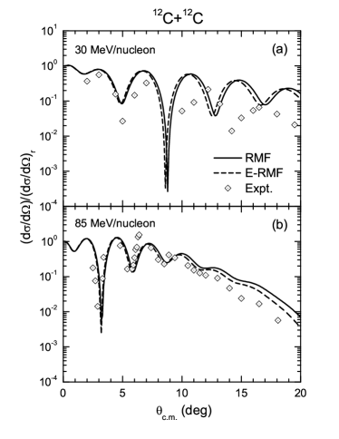
Figure 6: Differential cross-section for ¹²C+¹²C system: (a) at 30 MeV/nucleon of incident energy and (b) at 85 MeV/nucleon of incident energy. The experimental data are taken from buen84 .

Figure 7: Same as Fig. 6, but for ¹¹Li as projectile.

III.4 Differential cross-section

Results for elastic differential cross-section $\frac{(d\sigma/d\Omega)}{(d\sigma/d\Omega)_{r}}$ for the ¹²C+¹²C system have been shown in Fig. 6 at 30 MeV/nucleon as well as 85 MeV/nucleon of incident energies. We see that the elastic scattering angular distributions for ¹²C+¹²C, are better reproduced using E-RMF (G2 set) nuclear densities than RMF (SIG-OM) one while demanding conformity with experimental data buen84 . This example clearly shows the importance of nuclear densities and highlights the sensitivity of the experimental differential cross-section to details of nuclear structure. Results for the elastic scattering angular distributions for RIB projectiles have been shown in Fig. 7.

From the above study, it is interesting to observe that the two relativistic approaches give slightly different cross-sections which could be attributed to the different results obtained for ground state properties. Hence the details of structure information have to be considered crucial as they are well reflected in the reaction cross-sections. At low energy region (30 MeV/nucleon), both differential scattering cross-section (SIG-OM and G2) are similar to each other as shown in Fig. 6(a). The experimental trend is reproduced well using both the densities as input in the evaluation of differential cross-section. However, if one analyse the data at 85 MeV/nucleon as shown in Fig. 6(b), the values of $\frac{(d\sigma/d\Omega)}{(d\sigma/d\Omega)_{r}}$ obtained with both RMF and E-RMF approaches agree well with the experiment, both qualitatively and quantitatively.

Similar results of differential cross-section for exotic nuclei which are predicted as likely halo candidates, namely ¹¹Li, ¹¹Be and ¹⁴Be tan96 , with ¹²C as target nucleus is shown in Fig. 7 taking incident energies as 30 MeV/nucleon and 85 MeV/nucleon. In all these systems i.e. ¹¹Li+¹²C, ¹¹Be+¹²C, ¹⁴Be+¹²C, the differential cross-sections obtained with both, the RMF and the E-RMF densities are almost similar.

IV Summary

In summary, we have used the Glauber model to calculate nuclear reaction cross-section with densities obtained from RMF and E-RMF calculations using SIG-OM and G2 set of parameters respectively. We have seen that the calculation of total reaction cross-section can be performed well with the Glauber model using RMF and E-RMF nuclear densities as the main ingredient. The good quality of results shows that the nuclear reaction cross-section predictions from the Glauber model calculations using RMF and E-RMF nuclear densities will be helpful in more stringent analysis of the high energy reactions involving the nuclei on either side of the valley of $\beta$-stability. The comparison with the results of double folding potential analysis using the same RMF and E-RMF nuclear densities would be enriching our knowledge more in the low energy region in this regard.

While analysing the differential cross-section, we found that the E-RMF density suited well to reproduce the experimental data. The RMF basically fails for larger scattering angle with higher incident energy. This study clearly shows the importance of extending RMF to E-RMF formalism to reduce the central density of the target. Thus, from these calculations it is clear that the E-RMF theory not only describe the ground state and nuclear matter properties of the nuclei successfully, but also explains the nuclear reaction data quite well. Overall, these calculations give an excellent account for the existing experimental data for ground state properties namely, nuclear radii and binding energy as well as for nuclear reaction cross-section results. Further, it is hoped that such precise studies for cross-section calculations of exotic nuclei may also be very crucial in view of upcoming radioactive ion beam facilities.

References

- (1) A. Ozawa, T. Suzuki and I. Tanihata, Nucl. Phys. A693, 32 (2001).
- (2) D. T. Khoa, H. Sy Than, T. H. Nam, M. Grasso and N. V. Giai Phys. Rev. C69, 044605 (2004).
- (3) F. M. Nunes, N. C. Summers, A. M. Moro and A. M. Mukhamedzhanov, Proceedings of ’Nuclei at the limits’, ANL 26-30 July 2004; arXiv: nucl-th/0505046.
- (4) I. Tanihata, J. Phys. G22, 157 (1996).
- (5) I. Tanihata, H. Hamagaki, O. Hashimoto, Y. Shida, N. Yoshikawa, K. Sugimoto, O. Yamakawa, T. Kobayashi and N. Takahashi, Phys. Rev. Lett. 55, 2676 (1985).
- (6) T. Kobayashi, O. Yamakawa, K. Omata, K. Sugimoto, T. Shimoda, N. Takahashi and I. Tanihata, Phys. Rev. Lett. 60, 2599 (1988).
- (7) P. G. Hansen and B. Jonson, Europhys. Lett. 4, 409 (1989).
- (8) W. Mittig et al., Phys. Rev. Lett. 59, 1889 (1987).
- (9) K. Varga, S. C. Pieper, Y. Suzuki and R. B. Wiringa, Phys. Rev. C66, 034611 (2002).
- (10) B. Abu-Ibrahim, Y. Ogawa, Y. Suzuki and I. Tanihata, Comp. Phys. Comns. 151, 369 (2003).
- (11) R. J. Glauber, Lectures on Theoretical Physics, edited by W. E. Brittin and L. C. Dunham (Interscience, New York, 1959), Vol.1, p.315.
- (12) G. F. Bertsch, B. A. Brown and H. Sagawa, Phys. Rev. C39, 1154 (1989).
- (13) M. Y. H. Farag, Eur. Phys. J. C12, 1112 (2001).
- (14) A. Bhagwat and Y. K. Gambhir, Phys. Rev. C69, 014315 (2004); A. Bhagwat, Y. K. Gambhir and S. H. Patil, Eur. Phys. J. A8, 511 (2000); J. Phys. G27, B1 (2001).
- (15) B. K. Sharma, S. K. Patra, Raj K. Gupta, A. Shukla, P. Arumugam, P. D. Stevenson and Walter Greiner, J. Phys. G 32, 2089 (2006).
- (16) S. K. Patra and C. R. Praharaj, Phys. Rev. C44 (1991) 2552; Y. K. Gambhir, P. Ring and A. Thimet, Ann. Phys. (N.Y.) 198, 132 (1990).
- (17) B. D. Serot and J. D. Walecka, Int. J. Mod. Phys. E6, 515 (1997).
- (18) R. J. Furnstahl, B. D. Serot and H. B. Tang, Nucl. Phys. A598, 539 (1996); ibid A615, 441 (1997).
- (19) P. Arumugam, B. K. Sharma, P. K. Sahu, S. K. Patra, T. Sil, M. Centelles and X. Viñas, Phys. Lett. B601, 51 (2004).
- (20) M. Del Estal, M. Centelles, X. Viñas and S. K. Patra, Phys. Rev C63, 024314 (2001).
- (21) M. Del Estal, M. Centelles, X. Viñas and S. K. Patra, Phys. Rev. C63, 044321 (2001).
- (22) P. J. Karol, Phys. Rev. C11, 1203 (1975).
- (23) M. M. Haidari and M. M. Sharma, nucl-th/0702001.
- (24) G. Audi, A. H. Wapstra and C. Thibault, Nucl. Phys. A729, 337 (2003).
- (25) I. Angeli, At. Data and Nucl. Data Tables 87, 185 (2004).
- (26) Y. Ogawa, K. Yabana and Y. Suzuki, Nucl. Phys. A543, 722 (1992).
- (27) J. Chauvin, D. Lebrun and M. Buenerd, Phys. Rev. C28, 1970 (1983); M. Buenerd, A. Lounis, J. Chauvin, D. Lebrun, P. Martin, G. Duhamel, J.C. Gondrand and P.D. Saintignon, Nucl. Phys. A424, 313 (1984); J.Y. Hostachy et al, Nucl. Phys. A490, 441 (1988).
- (28) Yong-Xu Yang, Qing-Run Li and Wei-Qin Zhao, J. Phys. G28, 2561 (2002).
- (29) J. Jaros et al., Phys. Rev. C 18, 2273 (1978).
- (30) B. K. Sharma, P. Arumugam, A. Shukla and S. K. Patra Proceedings of Nuclear Structure Physics at extremes, H.P. University, Shimla, India (2005).