Isospin mixing and energy distributions in three-body decay

Abstract

The structure of the second 2⁺ resonance in ⁶Li is investigated with special emphasis on its isospin 0 components. The wave functions are computed in a three-body model ($\alpha$+$n$+$p$) using the hyperspherical adiabatic expansion method combined with complex scaling. In the decay into three free particles the symmetry conserving short-range interaction dominates at short distance whereas the symmetry breaking Coulomb interaction dominates at intermediate and large distances resulting in substantial isospin mixing. We predict the mixing and the energy distributions of the fragments after decay. Computations are consistent with available experiments. We conjecture that nuclear three-body decays frequently produce such large isospin mixing at large distance where the energy distributions are determined.

Introduction.

The spatial extension of halo states depends sensitively on their binding energy jen04 . The reason is that the outer particles forming the loosely bound halo are confined by an attraction or a barrier of moderate size. This sensitivity to the energy must be particularly important for resonances owing their existence to a confining barrier. For the same reason, due to the effect of the Coulomb interaction, the structure of isobaric analog resonances can be very different. This influence can also be reflected in mixing of different isospin components. For ordinary states the isospin mixing has been established to be in the range $10^{-4}$-$10^{-5}$ boh69 . For isobaric analogs to halo states the mixing could be substantially larger han93 .

Early theoretical investigations of decay of three-body analog halo states in light nuclei indicated that isospin is very well conserved suz91 ; ara95 . A very small isospin mixing is also deduced from the reduced measured branching ratio of decay of the highest known 2⁺ resonance in ⁶Li (with excitation energy of 5.37 MeV and associated to isospin 1) into the $\alpha$-deuteron two-body system deb71 ; wit75 (admixture of $8\cdot 10^{-3}$ or less). Nevertheless, isospin mixing in ⁶Li-states is also investigated in a number of reaction experiments ²H$(\alpha,\alpha)^{2}$H^∗ where ²H^∗ is the neutron-proton system in a spin singlet relative state which cannot be populated when isospin is conserved. Strong evidence is claimed for the formation of ²H^∗ which means substantial isospin mixing and especially when the incident energy is low wer81 ; gai88 ; nie92 . Reasonable agreement between measurements and simple model calculations can only be obtained with inclusion of both spin zero neutron-proton $s$-wave (²H^∗) and nucleon-$\alpha$ relative $d$-waves. Some of these authors wer81 suggest the large isospin mixture to be due to direct reactions bypassing the ⁶Li resonance, whereas others gai88 call for better methods for including the Coulomb interaction in three-body calculations.

Recent investigations emphasized that the structure of three-body resonances can change substantially from small to large distances gar05b ; gar05c ; gar05f . This means for instance that the amount of isospin may vary substantially with the (hyper)radial coordinate describing the wave function. In other words, the relative weights of different partial wave components can be very different from small to large distances, e.g. in ⁶Li ($\alpha$ + n + p) for neutron and proton in relative $s$-waves and in triplet or singlet spin states corresponding to $T=0$ or $T=1$, respectively. The absence of decay of the $2^{+}$ resonance in ⁶Li into the deuteron channel is not a direct evidence for a correspondingly small admixture of isospin 0. The dominant isospin 1 wave function at small distance can decay into continuum final states with isospin 0 provided the coupling is sufficiently strong. This is most likely at distances just outside the ranges of the short-range interactions where the Coulomb interaction still is substantial and completely dominating.

The purpose of the present letter is to investigate the isospin conservation in the 2⁺ three-body resonance in ⁶Li, that is the isobaric analog state of the corresponding 2⁺ resonance in ⁶He and ⁶Be, for which isospin zero components are forbidden. We start with a sketch of the necessary theoretical framework. We then discuss the structure of the resonance and present the final state energy distributions. We finish with a brief summary and the conclusions.

Theoretical framework.

Bound states and resonances are obtained with the hyperspherical adiabatic expansion method combined with complex scaling. These three-body wave functions $\Psi$ are then expressed as a linear combination of the complete set of functions $\{\Phi_{n}(\rho,\Omega)\}$ nie01

$$\Psi(\bm{x},\bm{y})=\frac{1}{\rho^{5/2}}\sum_{n}f_{n}(\rho)\Phi_{n}(\rho,\Omega)\;,$$ (1)

where $\rho$ is the hyperradius and the five hyperangles $\Omega=\{\alpha,\Omega_{x},\Omega_{y}\}$ can formally be chosen in any of the three Jacobi sets, or as we prefer the wave function can be given in terms of three Faddeev components each associated with one Jacobi set. Each of these Faddeev components are in turn expanded in partial waves with a basis of corresponding hyperspherical harmonic functions.

The functions $\Phi_{n}(\rho,\Omega)$ are the eigenfunctions of the angular part of the Faddeev equations, and the radial coefficients $f_{n}(\rho)$ are obtained from the coupled set of radial equations where the eigenvalues of the angular part enter as effective adiabatic potentials nie01 . Due to the complex scaling the wave functions fall off exponentially at large hyperradii for bound states and resonances with width-to-energy ratios less than twice the rotation angle.

The components of the solution directly contain information about the symmetry and hence about the isospin mixing, which can vary with hyperradius. This point has apparently not been appreciated in the old analyses deb71 ; wit75 . For instance, in ⁶Li ($n$+$p$+$\alpha$) the total isospin is obtained by coupling neutron and proton isospins to either 0 or 1. Components with both isospins are in principle permitted, like for instance $(\ell_{x},\ell_{y},L,S,J)=(0,2,2,0,2),(1,1,2,0,2)$, where $\ell_{x}$ and $\ell_{y}$ are orbital angular momenta related to the Jacobi coordinates $\bm{x}$ and $\bm{y}$ (with $\bm{x}$ proportional to the neutron-proton distance), and $L$, $S$ and $J$ are the total orbital, spin and total angular momenta. In fact these two components do contribute, and are coupled due to the presence of the $\alpha$-particle, which Coulomb interacts with the proton but not with the neutron. This can totally break the (isospin) symmetry if the symmetry breaking interaction is dominating as it is for large distances. Thus, small isospin mixing at small distance can be compatible with a very large isospin mixing at large distance.

The kinetic energy distribution of the fragments after decay of a resonance is, except for a phase-space factor, obtained as the absolute square of the total wave function in coordinate space for a large value of the hyperradius $\rho$, but where the five hyperangles are interpreted as in momentum space gar05c ; gar05f . After integration over the four hyperangles $(\Omega_{x},\Omega_{y})$ describing the directions of the two Jacobi momenta, $\bm{k}_{x}$ and $\bm{k_{y}}$, conjugate to $\bm{x}$ and $\bm{y}$, the probability distribution as function of $k_{y}^{2}\propto\cos^{2}\alpha$, where $\alpha$ is the fifth momentum hyperangle, is given by

$$P(k_{y}^{2})\propto P(\cos^{2}\alpha)\propto\sin(2\alpha)\int d\Omega_{x}d\Omega_{y}|\Psi(\rho,\alpha,\Omega_{x},\Omega_{y})|^{2}\;.$$ (2)

The kinetic energy of the third particle is proportional to $k_{y}^{2}\propto\cos^{2}\alpha$ which then gives the energy of the particle relative to its maximum possible energy in the decay process. These observables carry information about initial state and decay mechanisms.

Details of the calculations.

The 2⁺ resonance in ⁶Li has been computed using the same $\alpha$-nucleon interaction as in cob98 for ⁶He. For the neutron-proton potential we use the one in cob97 . Components with relative two-body orbital angular momenta up to 4 are considered. The main components included in the calculation are shown in table 1 (the first column labels the components). A proper choice of the maximum value of the hypermomentum ($K_{max}$) for each of them is crucial to obtain a correct convergence of the effective potentials at a sufficiently large distance. The $K_{max}$ value for the components 6 to 11 in the left part of table 1 is relatively large to ensure an accurate calculation of their contribution, since these are precisely the components with zero isospin ($T$ in the table) that are not allowed in ⁶He or ⁶Be. For the remaining components (not shown in the table) the $K_{max}$-value is at least 20.

Table 1: Components included for the $2^{+}$-state in ⁶Li. The left part refers to the first Jacobi set ($\bm{x}$ from neutron to proton), and the right part to the second and third Jacobi sets ($\bm{x}$ from one of the nucleons to the $\alpha$-particle). The first column numbers the different components.

	1st Jacobi set							2nd and 3rd Jacobi sets
	$\ell_{x}$	$\ell_{y}$	$L$	$s_{x}$	$S$	$K_{max}$	$T$	$\ell_{x}$	$\ell_{y}$	$L$	$s_{x}$	$S$	$K_{max}$
1	0	2	2	0	0	240	1	0	2	2	1/2	0	44
2	2	0	2	0	0	180	1	0	2	2	1/2	1	44
3	1	1	1	1	1	180	1	2	0	2	1/2	0	70
4	1	1	2	1	1	64	1	2	0	2	1/2	1	44
5	2	2	2	0	0	90	1	1	1	1	1/2	1	240
6	0	2	2	1	1	240	0	1	1	2	1/2	0	240
7	2	0	2	1	1	240	0	1	1	2	1/2	1	44
8	1	1	2	0	0	240	0	2	2	1	1/2	1	32
9	2	2	1	1	1	240	0	2	2	2	1/2	0	50
10	2	2	2	1	1	240	0	2	2	2	1/2	1	42
11	2	2	3	1	1	240	0	1	3	2	1/2	0	42

Figure 1: Outer panel: Real parts of the (complex scaled) effective adiabatic potentials for the 2⁺ resonance in ⁶Li. Inner panel: Real parts of the radial wave functions associated to the three most contributing effective potentials (indicated by the thick curves in the outer part).

The outer part of Fig.1 shows the real parts of the effective potentials obtained after use of the (complex scaled) hyperspheric adiabatic expansion method. The lowest effective potential converges towards the deuteron binding energy, and appears due to the inclusion of the components with zero isospin in the neutron-proton channel. These potentials are indistinguishable from the ones obtained when the basis size is reduced by a factor of two. This fact guaranties the convergence of the potentials at least up to 100 fm.

Calculation of the resonance wave function requires specification of the corresponding boundary condition. As shown in gar07 , a simple box boundary condition at a sufficiently large distance is enough to obtain a resonance wave function with the proper asymptotics. This requires extrapolation of the effective potentials for $\rho$ values beyond 100 fm. An expansion of the form $A/\rho+B/\rho^{2}+C/\rho^{3}+\cdots$ is used (except for the lowest one). The non-adiabatic coupling functions $P_{nn^{\prime}}(\rho)$ and $Q_{nn^{\prime}}(\rho)$ (see nie01 ) are extrapolated as $Q_{nn}(\rho)=A_{Q_{nn}}/\rho^{2}+B_{Q_{nn}}/\rho^{3}+C_{Q_{nn}}/\rho^{4}$ for diagonal $Q^{\prime}s$ (diagonal $P^{\prime}s$ are zero), and as $A_{P,Q}/\rho^{3}+B_{P,Q}/\rho^{4}+C_{P,Q}/\rho^{5}$ for the non-diagonal $P$’s and $Q$’s.

A box boundary condition at $\rho_{max}$=1000 fm gives rise to a 2⁺ resonance in ⁶Li with energy and width ($E_{R}$,$\Gamma_{R}$)=(1.67,0.51) MeV (5.37 MeV excitation energy), that agrees with the experimental value of ($E_{R}$,$\Gamma_{R}$)=(1.67$\pm$0.02,0.54$\pm$0.02) MeV ajz88 (the resonance energy is indicated in Fig.1 by the dashed line). However, the extrapolation used for the effective potentials implies that the asymptotics of the radial wave functions must be $F_{\xi}(\eta,\kappa\rho)-iG_{\xi}(\eta,\kappa\rho)$, where $\kappa=\sqrt{2mE/\hbar^{2}}$, $F_{\xi}$ and $G_{\xi}$ are the regular and irregular Coulomb functions, and the Coulomb charge $\eta$ and the index $\xi$ can be easily obtained from $A$, $B$, and $A_{Q_{nn}}$. When this asymptotic condition is imposed, a much smaller value of $\rho_{max}$ is enough to obtain the resonance wave function (but still $\rho_{max}>$100 fm, and the expansions of the effective potentials, $P^{\prime}s$, and $Q^{\prime}s$ are required).

Figure 2: Thick curves: Radial wave functions corresponding to the three most contributing effective potentials. Thin curves: Expected asymptotics ($F_{\xi}(\eta,\kappa\rho)-iG_{\xi}(\eta,\kappa\rho)$) from the extrapolated potentials for $\rho>$100 fm.

In the inner part of Fig.1 we show the real parts of the computed radial wave functions. A complex scaling angle of 0.10 rads has been used. To make the picture cleaner we only show the ones associated with the three most contributing effective potentials (thick curves in the outer part of the figure). It is important to note that the contribution from the lowest adiabatic potential, the one holding deuteron at large distances, is very small, providing about $10^{-3}$% of the norm, which is consistent with deb71 ; wit75 . It is also necessary to investigate whether the radial wave functions have already reached the asymptotic behaviour for $\rho<100$ fm, i.e., in the $\rho$-region where the calculation is purely numerical. This would mean the asymptotics given by the extrapolated effective potentials, $P^{\prime}s$, and $Q^{\prime}s$, is consistent with the numerical results.

This is tested in Fig.2, where the real and imaginary parts of the three most relevant radial wave functions (thick curves) are shown and compared to the expected asymptotics as given by the regular and irregular Coulomb functions, with Coulomb charges and indices computed numerically from the extrapolation of the potentials (thin curves). The matching between the numerical wave functions and the asymptotics is already very good at about 60 fm, clearly below the $\rho$-value (100 fm) from which the extrapolations are used. The labels 1, 2, and 3 refer to the deepest thick potential, intermediate thick potential, and repulsive thick potential in the outer part of Fig.1.

From the three-body wave function in Eq.(1), we define the total weight (as function of $\rho$) as:

$$W(\rho)=\int\sin^{2}\alpha\cos^{2}\alpha d\alpha d\Omega_{x}d\Omega_{y}|\Psi(\rho,\alpha,\Omega_{x},\Omega_{y})|^{2},$$ (3)

When writing $\Psi$ in the first Jacobi set ($\bm{x}$ from neutron to proton) we find, after integration over $\rho$ in Eq.(3), that roughly 82% of the weight is given by the three first components in the left part of table 1 (38%, 20%, and 24%), while the remaining 18% is distributed among the other components.

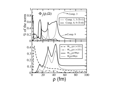
Figure 3: Top: Main contributions (as a function of $\rho$) of the components in the left part of table 1 to the eigenfunction $\Phi_{3}(\rho,\Omega)$ associated to the third adiabatic potential (thick repulsive potential in Fig.1). The thin and thick curves correspond to components associated to $T$=1 and $T$=0, respectively. Bottom: Weight of the $T$=1 (dashed) and $T$=0 (dot-dashed) components in the 2⁺ resonance wave function in ⁶Li (scaled by a factor 2.5). The thick and thin solid curves are the relative weight of the $T$=0 components and the relative weight of the 9^th component in the left part of table 1, respectively.

It is remarkable that the last components from 6 to 11 in the left part of table 1 (associated to zero isospin) accumulate about 4.5% of the integrated weight, most of it corresponding to component 9. This is due to the third adiabatic potential (repulsive thick potential in Fig.1), whose corresponding eigenfunction $\Phi_{3}(\rho,\Omega)$ is dominated at intermediate distances by the components with zero isospin in the neutron-proton channel. This is shown in the upper part of Fig.3, where we show, as a function of $\rho$, the main contributions to $\Phi_{3}(\rho,\Omega)$ from the components in the left part of table 1. The thick curves correspond to components 8 and 9 in the table ($T$=0). As observed in the figure, these components have a non-negligible weight at intermediate distances. In particular, component 9 gives a large contribution from 20 to 50 fm. Beyond 50 fm component 3 dominates ($T$=1), but still a 5% contribution from component 9 is present. The rapid transition in $\Phi_{3}$ from component 9 to 3 reflects that the isospin symmetry is totally broken, because only the Coulomb interaction is active. The lowest centrifugal barrier with $\ell_{y}$=1 is then abruptly preferred over $\ell_{y}$=2. At short distances, as seen on the bottom of Fig.2, the radial coefficient corresponding to the third adiabatic potential is negligible, but beyond 20 fm, the amplitude of $f_{3}(\rho)$ is similar to the one in $f_{1}(\rho)$ and $f_{2}(\rho)$.

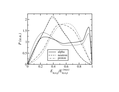
Figure 4: Thick curves: Energy distribution of the $\alpha$ (solid), neutron (dashed), and proton (dot-dashed) after decay of the 2⁺ resonance in ⁶Li. Thin curves: The same energy distributions after excluding the $T$=0 components.

Let us denote now by $W_{T=1}$ and $W_{T=0}$ the contributions to $W(\rho)$ in Eq.(3) from the $T$=1 and $T$=0 components in the three-body wave function, respectively. These contributions are shown (scaled by a factor 2.5) by the dashed and dot-dashed curves in the bottom part of Fig.3. At short distances the $T$=1 contribution clearly dominates, while $W_{T=0}$ becomes relevant at intermediate $\rho$’s. This is more clearly seen by the thick solid curve, that shows the relative weight of the $T$=0 components. From 20 to 50 fm this weight reaches up to 40% of the total. This region coincides with the one where $\Phi_{3}(\rho,\Omega)$ has a relevant contribution from the $T$=0 components (upper part of the figure). Beyond 50 fm $W_{T=0}$ stabilizes at about 10%. In the figure the thin curve shows the relative contribution to the total weight from component 9. This contribution gives most of the $T$=0 contribution, and governs the general behaviour of $W_{T=0}/W$.

The non-negligible isospin mixing found at large distances can be relevant for those observables sensitive to the asymptotic behaviour of the wave function, like for instance the energy distributions of the fragments after decay. In Fig.4 we show the $\alpha$ (solid), neutron (dashed), and proton (dot-dashed) energy distributions according to Eq.(2). The thick curves show the total distributions, while the thin ones give the same distributions when the $T$=0 components have been excluded. The results shown in the figure are very stable for $\rho$ values in Eq.(2) ranging from 65 to 85 fm. In particular the curves shown in the figure correspond to $\rho=75$ fm. As seen in the figure, inclusion of the $T$=0 components produce a visible change in the energy distributions, although the general behaviour of the distributions does not change.

Summary and conclusions.

We have investigated dynamic isospin mixing in nuclear resonances. We illustrate by the highest known $2^{+}$ resonance of the three-body system ⁶Li, where components with different isospin simultaneously can be present. The Coulomb interaction between $\alpha$-particle and proton is breaking the isospin symmetry and mixing isospins of 0 and 1. The isospin zero components essentially only appear in the neutron-proton continuum. The deuteron is populated in the decay by about $10^{-3}$%, that is consistent with the experimental upper limits deb71 ; wit75 . The amount of isospin zero is consistent with that found in experiments wer81 ; gai88 (up to 30% isospin mixing for low energies), while here the isospin mixing is due to the decay process and not direct reactions as suggested by these authors.

We have used the complex scaled, hyperspheric adiabatic expansion method with an extraordinary large basis for the components with zero isospin. The isospin content of the accurately computed resonance wave functions vary substantially from small to large distances. The relative isospin 0 contribution is small at small distances where the main contribution resides. This relative contribution reaches about 40% at intermediate distances, and stabilizes beyond 50 fm at roughly 10% of the total. The total contribution integrated over all distances of the isospin 0 components is about 4% which is much larger than for ordinary stable nuclei. This mechanism of dynamic isospin mixing is a common feature in decays of nuclear three- (or more-) body resonances.

References

- (1) A.S. Jensen, K. Riisager, D.V. Fedorov and E. Garrido, Rev. Mod. Phys. 76 (2004) 215.
- (2) A. Bohr and B. Mottelson, Nuclear Structure, vol I (Benjamin, New York, 1969) pp 31, 144, 171, 315, 331.
- (3) P.G. Hansen, A.S. Jensen and K. Riisager, Nucl. Phys. A560 (1993) 85.
- (4) Y. Suzuki and K. Yabana, Phys. Lett. B272 (1991) 173.
- (5) K. Arai, Y. Suzuki, and K. Varga, Phys. Rev. C51 (1995) 2488.
- (6) P.T. Debevec, G.T. Garvey and B.E Hingerty, Phys. Lett. B34 (1971) 497.
- (7) W. von Witsch, G.S. Mutchler and D. Miljanic, Nucl. Phys. A248 (1975) 485.
- (8) C. Werntz and F. Cannata, Phys. Rev. C24 (1981) 349.
- (9) N.O. Gaiser et al., Phys. Rev. C38 (1988) 1119.
- (10) P. Niessen et al., Phys. Rev. C45 (1992) 2570.
- (11) E. Garrido, D.V. Fedorov, A.S. Jensen and H.O.U. Fynbo, Nucl. Phys. A748 (2005) 39.
- (12) E. Garrido, D.V. Fedorov, A.S. Jensen and H.O.U. Fynbo, Nucl.Phys.A766 (2006) 74.
- (13) E. Garrido, D.V. Fedorov, H.O.U. Fynbo, and A.S. Jensen, Nucl. Phys. A781 (2007) 387.
- (14) E. Nielsen, D.V. Fedorov, A.S. Jensen and E. Garrido, Phys. Rep. 347 (2001) 373.
- (15) A. Cobis, D.V. Fedorov, and A.S. Jensen, Phys. Rev. C58 (1998) 1403.
- (16) A. Cobis, A.S. Jensen, and D.V. Fedorov, J. Phys. G23 (1997) 401.
- (17) E.Garrido, D.V. Fedorov, and A.S. Jensen, submitted for publication, nucl-th/0701040.
- (18) F. Ajzenberg-Selove, Nucl. Phys. A 490 (1988) 1.