Monopole Excitation to Cluster States

Abstract

We discuss strength of monopole excitation of the ground state to cluster states in light nuclei. We clarify that the monopole excitation to cluster states is in general strong as to be comparable with the single particle strength and shares an appreciable portion of the sum rule value in spite of large difference of the structure between the cluster state and the shell-model-like ground state. We argue that the essential reasons of the large strength are twofold. One is the fact that the clustering degree of freedom is possessed even by simple shell model wave functions. The detailed feature of this fact is described by the so-called Bayman-Bohr theorem which tells us that SU(3) shell model wave function is equivalent to cluster model wave function. The other is the ground state correlation induced by the activation of the cluster degrees of freedom described by the Bayman-Bohr theorem. We demonstrate, by deriving analytical expressions of monopole matrix elements, that the order of magnitude of the monopole strength is governed by the first reason, while the second reason plays a sufficient role in reproducing the data up to the factor of magnitude of the monopole strength. Our explanation is made by analysing three examples which are the monopole excitations to the $0^{+}_{2}$ and $0^{+}_{3}$ states in ¹⁶O and the one to the $0^{+}_{2}$ state in ¹²C. The present results imply that the measurement of strong monopole transitions or excitations is in general very useful for the study of cluster states.

I Introduction

The monopole transitions from cluster states to ground states in light nuclei are rather large in comparison with the single particle strength. For example in ¹⁶O the monopole matrix elements $M({\rm E0})$ between the ground state and the first and second excited $0^{+}$ states at $E_{x}$ = 6.05 MeV and 12.05 MeV which are known to have ¹²C+$\alpha$ cluster structure supple ; hoik ; suzuki are $3.55\pm 0.21$ fm² and $4.03\pm 0.09$ fm² ajzen86 , respectively. Also in ¹²C the $M({\rm E0})$ value between the ground state and the first excited $0^{+}$ state at $E_{x}$ = 7.66 MeV (so-called Hoyle state Hoyle ) which is known to have a $3\alpha$ cluster structure supple is $5.4\pm 0.2$ fm² ajzen86 . A rough estimate of the single particle strength $\langle u_{f}(r)|r^{2}|u_{i}(r)\rangle$ is $(3/5)R^{2}\sim 5.4~{}{\rm fm}^{2}$ for $p$- and $sd$-shell nuclei ($R\sim 3.0$ fm). This estimation formula is obtained under the uniform-density approximation of $u(r)\sim\sqrt{3/R^{3}}$ for $u_{f}(r)$ and $u_{i}(r)$ with $R$ standing for the nuclear radius. The energy weighted strengths of the above mentioned monopole transitions give an appreciable portion of the sum rule values: in ¹⁶O they are about 3 $\%$ and 8 % for $0^{+}_{2}$ and $0^{+}_{3}$, respectively, and in ¹²C about 16 % for $0^{+}_{2}$ (see Appendix A). Recently Kawabata and his collaborators have studied the excited states of ¹¹B by performing ${{}^{11}{\rm B}}(d,d^{\prime})$ reaction and they concluded that the third $3/2^{-}$ state at $E_{x}$ = 8.56 MeV has a $2\alpha+t$ cluster structure kawabata . Among many reasons for this conclusion, one is a large monopole strength for the third $3/2^{-}$ state which is of similar value to the monopole strength for the second $0^{+}$ state in ¹²C, and another is that the AMD (antisymmetrized molecular dynamics) calculation kawabata as well as the $2\alpha+t$ OCM (orthogonality condition model) calculation yamada07 have reproduced the large monopole strength and have assigned loosely bound $2\alpha+t$ cluster structure to the third $3/2^{-}$ state.

The single particle estimate of the monopole transition is based on the assumption that the excited state has a one-particle one-hole excitation from the ground state. However, the cluster structure is very different from the shell-model-like structure of the ground state, and its state is described as a superposition of many-particle many-hole configurations when it is expanded by shell model configurations. This means that in the excited state with a cluster structure, the component of a one-particle one-hole excitation from the ground state configuration is expected to be very small. Therefore the observation of rather large monopole strengths for cluster states which are comparable with single particle strength looks not to be easy to explain. The ¹²C+$\alpha$ OCM calculation suzuki for ¹⁶O and $3\alpha$ RGM (resonating group method) calculation kami ; uega , however, have reproduced rather well the experimental data of the monopole transitions. No explicit and detailed analyses of the reason why the cluster models reproduce plausibly the experimental data have been presented so far as long as we know. There should exist underlying physics in the monopole transition strengths in light nuclei.

The purpose of this paper is to clarify the basic reasons why monopole transition strength between a cluster state and the ground state in light nuclei is generally rather large in comparison with the single particle strength and shares an appreciable portion of the sum rule value, in spite of the large difference of structure between the initial and final states. We analyse the above-mentioned three cases of monopole transisions in ¹⁶O and ¹²C, namely the monopole transitions between the ground state and the first and second excited $0^{+}$ states in ¹⁶O, and the monopole transition between the ground state and the first excited $0^{+}$ state in ¹²C. By using these analyses we will show that there are two basic reasons for the generally large strength of monopole transitions. The first reason is the fact that the clustering degree of freedom is possessed even by simple shell model wave functions. The detailed feature of this fact is described by the so-called Bayman-Bohr theorem BB . This theorem tells us that the SU(3) shell model wave function elliott58 describing the ground state is in most cases equivalent to the cluster-model wave function discussed by Wildermuth and Kanellopoulos Wildermuth . Thus we can see what kinds of clustering degrees of freedom are embedded in the ground state. For example the doubly closed-shell wave function of the ¹⁶O ground state (total quanta $N_{TOT}=12$) which is just the SU(3) shell model wave function with $(\lambda,\mu)=(0,0)$ is equivalent to a ¹²C + $\alpha$ cluster-model wave function with $N_{TOT}=12$. This means that the ground-state wave function of ¹⁶O originally has a ¹²C+$\alpha$ clustering degree of freedom. The second reason is the ground state correlation induced by the activation of the cluster degrees of freedom described by the Bayman-Bohr theorem. In the case of the above example of the ¹⁶O ground state, the ground state correlation is due to the ¹²C + $\alpha$ clustering degrees of freedom. As was explained, the first and second excited $0^{+}$ states of ¹⁶O are the cluster states with ¹²C + $\alpha$ structure. These cluster states are formed just by the excitation of the ¹²C + $\alpha$ clustering degree of freedom which is already existent in the ground state. Therefore it is quite reasonable that the large strength of the monopole transition between the ground state and the first and second excited $0^{+}$ states is explained by the above-mentioned first and second reasons. We will demonstrate, by deriving analytical expressions of monopole matrix elements, that the order of magnitude of the monopole strength is governed by the first reason, while the second reason plays a sufficient role in reproducing the data up to the factor of magnitude of the monopole strength.

In the present paper we discuss the details of the first and second reasons for ¹⁶O and ¹²C. In the case of ¹⁶O, we make use of the microscopic ¹²C + $\alpha$ cluster wave function, while in the case of ¹²C, we discuss the problem by using the so-called THSR wave function tohsaki ; funaki . Our results mean that the measurement of strong monopole transitions provides us in general with a very useful tool for the experimental study of cluster states as has been practiced in Ref. kawabata .

The present paper is organized as follows. In Sec. II we derive analytical expressions of the monopole matrix elements between the ground state and ¹²C+$\alpha$ cluster states in ¹⁶O and those between the ground state and $3\alpha$ cluster state in ¹²C, by using the Bayman-Bohr theorem. In Sec. III we discuss the effect of the ground state correlation on the monopole transitions from the ¹²C$+\alpha$ cluster states in ¹⁶O, and those from the $3\alpha$ cluster state in ¹²C. In Sec. IV we give discussions and summary.

II Monopole Transition and Bayman-Bohr Theorem

II.1 Monopole transition from two-cluster states in ¹⁶O

We discuss the following two observed values of the monopole transition matrix element in ¹⁶O: One is $M({\rm E0})=3.55\pm 0.21$ fm² between the ground state ($0^{+}_{1}$) and the first excited $0^{+}$ state ($0^{+}_{2}$) at $E_{x}$ = 6.05 MeV, and the other is $M({\rm E0})=4.03\pm 0.09$ fm² between the ground state and the excited $0^{+}$ state ($0^{+}_{3}$) at $E_{x}$ = 12.05 MeV. These excited $0^{+}$ states are known to have ¹²C+$\alpha$ structures supple ; hoik ; suzuki . In this section, we explain that the order of magnitude of these $M({\rm E0})$ values comparable with the single nucleon strength is explained to come from the fact that the doubly closed shell wave function already contains in it the ¹²C+$\alpha$ clustering degree of freedom. For this purpose we derive analytical expressions of these monopole matrix elements by the use of the Bayman-Bohr theorem.

The nuclear SU(3) model or Elliott model elliott58 is known to describe well ground states of light nuclei. The ground state of ¹⁶O has a doubly closed shell structure of $0s$ and $0p$ orbits which belongs to the SU(3) irreducible representation $(\lambda,\mu)=(0,0)$. This doubly closed shell model wave function with the nucleon size parameter $\nu_{N}=M\omega/2\hbar$ ($M$: nucleon mass) is equivalent to a cluster wave function of ¹²C + $\alpha$ configuration, according to the Bayman-Bohr theorem,

$$\frac{1}{\sqrt{16!}}\det|(0s)^{4}(0p)^{12}|=N_{g}\frac{1}{\sqrt{{}_{16}C_{4}}}{\cal A}\{[{\cal R}_{4}(\mbox{\boldmath$r$},3\nu_{N})\phi({}^{12}{\rm C})]_{(0,0)}\phi(\alpha)\}\phi_{G}(\mbox{\boldmath$r$}_{G}),$$ (1)

$$[{\cal R}_{4}(\mbox{\boldmath$r$},3\nu_{N})\phi({}^{12}{\rm C})]_{(\lambda,\mu)=(0,0)}=\sum_{L=0,2,4}C_{L}\ [{\cal R}_{4L}(\mbox{\boldmath$r$},3\nu_{N})\phi_{L}({}^{12}{\rm C})]_{J=0},$$ (2)

$$\phi_{G}(\mbox{\boldmath$r$}_{G})=\left(\frac{32\nu_{N}}{\pi}\right)^{3/4}\exp\left(-16\nu_{N}\mbox{\boldmath$r$}_{G}^{2}\right),\ \ \mbox{\boldmath$r$}_{\rm G}=\frac{1}{16}\sum_{i=1}^{16}\mbox{\boldmath$r$}_{i}$$ (3)

$$C_{L}=\langle(4,0)L,(0,4)L||(0,0)0\rangle,\ \ {}_{16}C_{4}=\frac{16!}{12!4!}.$$ (4)

Here $\phi(\alpha)$ and $\phi_{L}({}^{12}{\rm C})$ stand for the internal wave function of $\alpha$ cluster with the $(0s)^{4}$ configuration and internal wave function of ¹²C with angular momentum $L$, respectively. $\phi_{G}$ denotes the center-of-mass wave function of ¹⁶O, which can be separated from the internal wave function as is written in Eq. (1). The relative wave function between the $\alpha$ and ¹²C clusters is presented by the harmonic oscillator wave function ${\cal R}_{NLm}(\mbox{\boldmath$r$},\beta)=R_{NL}(r,\beta)Y_{Lm}({\hat{\mbox{\boldmath$r$}}})$ with the oscillator quanta $N=4$ [nodal number $n=(N-L)/2$] and size parameter $\beta=3\nu_{N}$, where $r$ is the relative coordinate between the center-of-masses of $\alpha$ and ¹²C clusters. It is noted that ${\cal R}_{4L}(\mbox{\boldmath$r$},3\nu_{N})$ and $\phi_{L}({}^{12}{\rm C})$ belong to the SU(3) irreducible representations $(\lambda,\mu)=(4,0)$ and (0,4), respectively. Equation (2) means that these representations are coupled to the SU(3) scalar representation $(\lambda,\mu)=(0,0)$. ${\cal A}$ is the nucleon antisymmetrizer between ¹²C and $\alpha$ cluster, $N_{g}$ is the normalization constant, and $C_{L}$ is the reduced Clebsch-Gordan coefficient of SU(3) group for the SU(3) vector coupling $(4,0)\times(0,4)\rightarrow(0,0)$.

The doubly closed shell model wave function of ¹⁶O has the total number of the oscillator quanta $N_{TOT}=12$ and is only one possible wave function allowed for $N_{TOT}=12$. Since all three wave functions of ¹⁶O, ${\cal A}\{[{\cal R}_{4L}(\mbox{\boldmath$r$},3\nu_{N})\phi_{L}({}^{12}{\rm C})]_{J=0}\phi(\alpha)\}$ for $L$=0, 2, and 4, have the total quanta $N_{TOT}=12$, they are necessarily equivalent to the doubly closed shell model wave function $\Phi_{CS}$ and represent the internal wave function of the ¹⁶O ground state (see also Appendix B),

$$|{0^{+}_{1}}\rangle = \Phi_{CS}\equiv{\frac{1}{\sqrt{16!}}\det|(0s)^{4}(0p)^{12}|}\times[\phi_{G}(\mbox{\boldmath$r$}_{G})]^{-1}$$ (5)

$$= N_{g0}\frac{1}{\sqrt{{}_{16}C_{4}}}{\cal A}\{[{\cal R}_{40}(\mbox{\boldmath$r$},3\nu_{N})\phi_{L=0}({}^{12}{\rm C})]_{J=0}\phi(\alpha)\}$$ (6)

$$= N_{g2}\frac{1}{\sqrt{{}_{16}C_{4}}}{\cal A}\{[{\cal R}_{42}(\mbox{\boldmath$r$},3\nu_{N})\phi_{L=2}({}^{12}{\rm C})]_{J=0}\phi(\alpha)\}$$ (7)

$$= N_{g4}\frac{1}{\sqrt{{}_{16}C_{4}}}{\cal A}\{[{\cal R}_{44}(\mbox{\boldmath$r$},3\nu_{N})\phi_{L=4}({}^{12}{\rm C})]_{J=0}\phi(\alpha)\},$$ (8)

where $N_{g0}$, $N_{g2}$, and $N_{g4}$ denote the normalization constants. It is important to recognize the implication of these relations of Eqs. (1), and (6)$\sim$(8). They imply that the ground state of ¹⁶O can be excited not only through single particle degrees of freedom by promoting nucleons from $0s$ and $0p$ orbits to higher orbits, but also through cluster degrees of freedom by exciting the ¹²C$-$$\alpha$ relative motion from ${\cal R}_{4L}(\mbox{\boldmath$r$},3\nu_{N})$ state to higher nodal states. The latter characteristic is an essential point to understand why the monopole transition matrix elements to cluster states are in general large.

II.1.1 Monopole transition between $0_{1}^{+}$ and $0_{2}^{+}$ states

The $0_{2}^{+}$ state of ¹⁶O is known to have a loosely bound ¹²C+$\alpha$ structure, in which the dominant component of ¹²C is the ground state supple ; hoik ; suzuki . Thus we express the $0_{2}^{+}$ wave function as

$$|0_{2}^{+}\rangle=N_{I}\frac{1}{\sqrt{{}_{16}C_{4}}}{\cal A}\{\chi_{0}(\mbox{\boldmath$r$})\phi_{L=0}({}^{12}{\rm C})\phi(\alpha)\},$$ (9)

where $N_{I}$ represents the normalization constant. By expanding $\chi_{0}(\mbox{\boldmath$r$})$ in terms of harmonic oscillator functions, we have

$$|0^{+}_{2}\rangle = \sum_{N=6}^{\infty}\eta_{N}\Phi_{N},$$ (10)

$$\Phi_{N} = \frac{1}{\sqrt{\tau_{0,N}}}\frac{1}{\sqrt{{}_{16}C_{4}}}{\cal A}\{R_{N0}(r,3\nu_{N})Y_{00}(\hat{\mbox{\boldmath$r$}})\phi_{L=0}({}^{12}{\rm C})\phi(\alpha)\},$$ (11)

$$\tau_{0,N} \equiv \langle{\cal R}_{N0}(\mbox{\boldmath$r$},3\nu_{N})\phi_{L=0}({}^{12}{\rm C})\phi(\alpha)|{\cal A}\{{\cal R}_{N0}(\mbox{\boldmath$r$},3\nu_{N})\phi_{L=0}({}^{12}{\rm C})\phi(\alpha)\}\rangle.$$ (12)

It should be noted that $\Phi_{N}$ are normalized. Also it should be noted that $\Phi_{N=4}$ is just the doubly closed shell wave function as is seen in Eq. (6), $|0_{1}^{+}\rangle=\Phi_{N=4}$.

Since both $0_{1}^{+}$ and $0_{2}^{+}$ states have the total isospin $T=0$, the monopole transition matrix element $M({\rm E0})$ is

$$M({\rm E0},0_{2}^{+}-0_{1}^{+})=\langle 0_{1}^{+}|\sum_{i=1}^{16}\frac{1}{2}(1+\tau_{3i})(\mbox{\boldmath$r$}_{i}-\mbox{\boldmath$r$}_{G})^{2}|0_{2}^{+}\rangle$$

$$\ \ =\langle 0_{1}^{+}|\frac{1}{2}\sum_{i=1}^{16}(\mbox{\boldmath$r$}_{i}-\mbox{\boldmath$r$}_{G})^{2}|0_{2}^{+}\rangle$$

$$\ \ =\eta_{6}\langle\Phi_{N=4}|\frac{1}{2}\sum_{i=1}^{16}(\mbox{\boldmath$r$}_{i}-\mbox{\boldmath$r$}_{G})^{2}|\Phi_{N=6}\rangle.$$ (13)

Here $\mbox{\boldmath$r$}_{G}$ stands for the total center-of-mass coordinate, $\mbox{\boldmath$r$}_{\rm G}=(1/16)\sum_{i=1}^{16}\mbox{\boldmath$r$}_{i}$. The last equality is because $\sum_{i=1}^{16}(\mbox{\boldmath$r$}_{i}-\mbox{\boldmath$r$}_{G})^{2}\Phi_{N=4}$ can not have more than 2$\hbar\omega$ excitation than $\Phi_{N=4}$. Then we have

$$M({\rm E0},0_{2}^{+}-0_{1}^{+})=\frac{\eta_{6}}{2}\frac{1}{\sqrt{\tau_{0,4}\tau_{0,6}}}$$

$$\ \ \ \times\langle{\cal R}_{40}(\mbox{\boldmath$r$},3\nu_{N})\phi_{L=0}({}^{12}{\rm C})\phi(\alpha)|{\cal A}\{(\sum_{i=1}^{16}(\mbox{\boldmath$r$}_{i}-\mbox{\boldmath$r$}_{\rm G})^{2}){\cal R}_{60}(\mbox{\boldmath$r$},3\nu_{N})\phi_{L=0}({}^{12}{\rm C})\phi(\alpha)\}\rangle$$

$$\ \ =\frac{\eta_{6}}{2}\frac{1}{\sqrt{\tau_{0,4}\tau_{0,6}}}\langle{\cal R}_{40}(\mbox{\boldmath$r$},3\nu_{N})\phi_{L=0}({}^{12}{\rm C})\phi(\alpha)|{\cal A}\{\frac{12\times 4}{16}\mbox{\boldmath$r$}^{2}{\cal R}_{60}(\mbox{\boldmath$r$},3\nu_{N})\phi_{L=0}({}^{12}{\rm C})\phi(\alpha)\}\rangle..$$ (14)

In obtaining Eq. (14), we first used the identity

$$\sum_{i=1}^{16}(\mbox{\boldmath$r$}_{i}-\mbox{\boldmath$r$}_{G})^{2}=\sum_{i\in{{}^{12}{\rm C}}}(\mbox{\boldmath$r$}_{i}-\mbox{\boldmath$r$}_{C})^{2}+\sum_{i\in\alpha}(\mbox{\boldmath$r$}_{i}-\mbox{\boldmath$r$}_{\alpha})^{2}+\frac{12\times 4}{16}\mbox{\boldmath$r$}^{2},$$ (15)

where $\mbox{\boldmath$r$}_{\rm C}$ and $\mbox{\boldmath$r$}_{\alpha}$ express the center-of-mass coordinate of ¹²C and $\alpha$, respectively. We then used the following relations,

$$\langle{\cal R}_{40}(\mbox{\boldmath$r$},3\nu_{N})\phi_{L=0}({}^{12}{\rm C})\phi(\alpha)|{\cal A}\{{\cal R}_{60}(\mbox{\boldmath$r$},3\nu_{N})\ (\sum_{i\in{}^{12}{\rm C}}(\mbox{\boldmath$r$}_{i}-\mbox{\boldmath$r$}_{\rm C})^{2})\phi_{L=0}({}^{12}{\rm C})\ \phi(\alpha)\}\rangle=0,$$ (16)

$$\langle{\cal R}_{40}(\mbox{\boldmath$r$},3\nu)\phi_{L=0}({}^{12}{\rm C})\phi(\alpha)|{\cal A}\{{\cal R}_{60}(\mbox{\boldmath$r$},3\nu_{N})\ \phi_{L=0}({}^{12}{\rm C})\ (\sum_{i\in\alpha}(\mbox{\boldmath$r$}_{i}-\mbox{\boldmath$r$}_{\alpha})^{2})\phi(\alpha)\}\rangle=0.$$ (17)

These relations can be easily proved by counting the total numbers of oscillator quanta of the bra and ket functions. First, the number of the oscillator quanta of ${\cal R}_{60}(\mbox{\boldmath$r$},3\nu_{N})$ is larger than that of ${\cal R}_{40}(\mbox{\boldmath$r$},3\nu_{N})$ by 2. Second, the number of the oscillator quanta of $(\sum_{i}(\mbox{\boldmath$r$}_{i}-\mbox{\boldmath$r$}_{\rm C})^{2})\phi_{L=0}({}^{12}{\rm C})$ can not be smaller than that of $\phi_{L=0}({}^{12}{\rm C})$ because $\phi_{L=0}({}^{12}{\rm C})$ has the smallest number of the oscillator quanta in the ¹²C ($N=Z=6$) system. Similarly, the number of the oscillator quanta of $(\sum_{i}(\mbox{\boldmath$r$}_{i}-\mbox{\boldmath$r$}_{\alpha})^{2})\phi(\alpha)$ can not be smaller than that of $\phi(\alpha)$. Therefore in each of Eqs. (16) and (17), the ket function has larger total number of the oscillator quanta than that of the bra function at least by 2, which leads to the orthogonality of the bra and ket functions.

Now we expand $(12\times 4/16)\mbox{\boldmath$r$}^{2}{\cal R}_{60}(\mbox{\boldmath$r$},3\nu_{N})$ in Eq. (14) in terms of the harmonic oscillator function

$$\frac{12\times 4}{16}\mbox{\boldmath$r$}^{2}{\cal R}_{60}(\mbox{\boldmath$r$},3\nu_{N})=\sum_{N}\langle{\cal R}_{N0}(\mbox{\boldmath$r$},3\nu_{N})|\frac{12\times 4}{16}\mbox{\boldmath$r$}^{2}|{\cal R}_{60}(\mbox{\boldmath$r$},3\nu_{N})\rangle\ {\cal R}_{N0}(\mbox{\boldmath$r$},3\nu_{N}).$$ (18)

By inserting Eq. (18) into Eq. (14) we obtain

$$M({\rm E0},0_{2}^{+}-0_{1}^{+}) = \frac{\eta_{6}}{2}\frac{1}{\sqrt{\tau_{0,4}\tau_{0,6}}}\langle{\cal R}_{40}(\mbox{\boldmath$r$},3\nu_{N})|\frac{12\times 4}{16}\mbox{\boldmath$r$}^{2}|{\cal R}_{60}(\mbox{\boldmath$r$},3\nu_{N})\rangle$$ (19)

$$\ \ \times\langle{\cal R}_{40}(\mbox{\boldmath$r$},3\nu_{N})\phi_{L=0}({}^{12}{\rm C})\phi(\alpha)|{\cal A}\{{\cal R}_{40}(\mbox{\boldmath$r$},3\nu_{N})\phi_{L=0}({}^{12}{\rm C})\phi(\alpha)\}\rangle$$

$$= \frac{\eta_{6}}{2}\sqrt{\frac{\tau_{0,4}}{\tau_{0,6}}}\langle{\cal R}_{40}(\mbox{\boldmath$r$},3\nu_{N})|\frac{12\times 4}{16}\mbox{\boldmath$r$}^{2}|{\cal R}_{60}(\mbox{\boldmath$r$},3\nu_{N})\rangle$$

$$= \frac{\eta_{6}}{2}\sqrt{\frac{\tau_{0,4}}{\tau_{0,6}}}\langle R_{40}(r,3\nu_{N})|\frac{12\times 4}{16}r^{2}|R_{60}(r,3\nu_{N})\rangle.$$

Here we note the following relation

$$\langle R_{40}(r,3\nu_{N})|\frac{12\times 4}{16}r^{2}|R_{60}(r,3\nu_{N})\rangle=\langle R_{40}(r,\nu_{N})|r^{2}|R_{60}(r,\nu_{N})\rangle,$$ (20)

where $R_{N0}(r,\nu_{N})$ is the harmonic oscillator radial function of single nucleon with the nucleon size parameter $\nu_{N}$. It is noted here that the matrix elements for calculating the single particle E0 matrix element in ¹⁶O are $\langle R_{00}(r,\nu_{N})|r^{2}|R_{20}(r,\nu_{N})\rangle$ and $\langle R_{11}(r,\nu_{N})|r^{2}|R_{31}(r,\nu_{N})\rangle$ which are a few times smaller than the present $\langle R_{40}(r,\nu_{N})|r^{2}|R_{60}(r,\nu_{N})\rangle$ as shown below,

$$\langle R_{00}(r,\nu_{N})|r^{2}|R_{20}(r,\nu_{N})\rangle = \sqrt{\frac{3}{8}}\frac{1}{\nu_{N}},\ \ \ \langle R_{11}(r,\nu_{N})|r^{2}|R_{31}(r,\nu_{N})\rangle=\sqrt{\frac{5}{8}}\frac{1}{\nu_{N}},$$ (21)

$$\langle R_{40}(r,\nu_{N})|r^{2}|R_{60}(r,\nu_{N})\rangle = \sqrt{\frac{21}{8}}\frac{1}{\nu_{N}}.$$ (22)

The reason why the number of oscillator quanta of the relative wave function is higher than those of the single particle wave functions is due to the Fermi statistics of nucleons.

The final analytical formula of $M({\rm E0},0_{2}^{+}-0_{1}^{+})$ is expressed as follows,

$$M({\rm E0},0_{2}^{+}-0_{1}^{+})=\frac{1}{2}\sqrt{\frac{\tau_{0,4}}{\tau_{0,6}}}\eta_{6}\langle R_{40}(r,\nu_{N})|r^{2}|R_{60}(r,\nu_{N})\rangle.$$ (23)

This analytical expression of $M({\rm E0},0_{2}^{+}-0_{1}^{+})$ is our desired result. It explains clearly why $M({\rm E0},0_{2}^{+}-0_{1}^{+})$ has a comparable magnitude as the single nucleon E0 matrix element. The factor $\langle R_{40}(r,\nu_{N})|r^{2}|R_{60}(r,\nu_{N})\rangle$ is a few times larger than the single nucleon E0 matrix elements $\langle R_{00}(r,\nu_{N})|r^{2}|R_{20}(r,\nu_{N})\rangle$ and $\langle R_{11}(r,\nu_{N})|r^{2}|R_{31}(r,\nu_{N})\rangle$, while the factor $\eta_{6}$ works to make the E0 value smaller.

II.1.2 Monopole transition between $0_{1}^{+}$ and $0_{3}^{+}$ states

The $0_{3}^{+}$ state of ¹⁶O at $E_{x}$ = 12.05 MeV is known to have also a ¹²C + $\alpha$ structure like the $0_{2}^{+}$ state supple ; suzuki . The ¹²C cluster in the $0_{3}^{+}$ state, however, is not mainly in its ground state like in $0_{2}^{+}$ state but dominantly in its excited $2^{+}$ state at $E_{x}$ = 4.44 MeV. Thus we can express the $0_{3}^{+}$ wave function in a good approximation as

$$|0_{3}^{+}\rangle=N_{II}\frac{1}{\sqrt{{}_{16}C_{4}}}{\cal A}\{[\chi_{2}(\mbox{\boldmath$r$})\phi_{L=2}({}^{12}{\rm C})]_{J=0}\phi(\alpha)\}.$$ (24)

Like in the case of $0_{2}^{+}$ state, we expand $\chi_{2}(\mbox{\boldmath$r$})$ in terms of harmonic oscillator wave functions and we obtain

$$|0^{+}_{3}\rangle = \sum_{N=6}^{\infty}\zeta_{N}\Psi_{N},$$ (25)

$$\Psi_{N} = \frac{1}{\sqrt{\tau_{2,N}}}\frac{1}{\sqrt{{}_{16}C_{4}}}{\cal A}\{[{\cal R}_{N2}(\mbox{\boldmath$r$},3\nu_{N})\phi_{L=2}({}^{12}{\rm C})]_{J=0}\phi(\alpha)\},$$ (26)

$$\tau_{2,N} \equiv \langle[{\cal R}_{N2}(\mbox{\boldmath$r$},3\nu_{N})\phi_{L=2}({}^{12}{\rm C})]_{J=0}\phi(\alpha)|{\cal A}\{[{\cal R}_{N2}(\mbox{\boldmath$r$},3\nu_{N})\phi_{L=2}({}^{12}{\rm C})]_{J=0}\phi(\alpha)\}\rangle.$$ (27)

It should be noted that $\Psi_{N}$ are normalized. Also it should be noted that $\Psi_{N=4}$ is just the doubly closed shell wave function as is seen in Eq. (7), $|0_{1}^{+}\rangle=\Psi_{N=4}$.

The calculation of the monopole transition matrix element $M({\rm E0},0_{3}^{+}-0_{1}^{+})$ can be made in the same manner as that of $M({\rm E0},0_{2}^{+}-0_{1}^{+})$ in the previous section, although we use Eq. (7) for the $0^{+}_{1}$ state of ¹⁶O,

$$M({\rm E0},0_{3}^{+}-0_{1}^{+})=\langle 0_{1}^{+}|\frac{1}{2}\sum_{i=1}^{16}(\mbox{\boldmath$r$}_{i}-\mbox{\boldmath$r$}_{\rm G})^{2}|0_{3}^{+}\rangle$$

$$\ \ =\frac{1}{2}\sqrt{\frac{\tau_{2,4}}{\tau_{2,6}}}\zeta_{6}\langle R_{42}(r,\nu_{N})|r^{2}|R_{62}(r,\nu_{N})\rangle,$$ (28)

where

$$\langle R_{42}(r,\nu_{N})|r^{2}|R_{62}(r,\nu_{N})\rangle=\frac{3}{2}\frac{1}{\nu_{N}}.$$ (29)

The analytical expression of $M({\rm E0},0_{3}^{+}-0_{1}^{+})$ in Eq. (28) is our another desired result. Like in the case of $M({\rm E0},0_{2}^{+}-0_{1}^{+})$, it explains clearly why $M({\rm E0},0_{3}^{+}-0_{1}^{+})$ has also a comparable magnitude as the single nucleon E0 matrix element.

II.1.3 Wave function which absorbs total monopole strength from the doubly closed shell

The wave function $\Phi_{(2,0)}$ which absorbs total monopole strength from the doubly closed shell wave function $\Phi_{CS}$ is given by

$$\Phi_{(2,0)} = N_{(2,0)}(1-|\Phi_{CS}\rangle\langle\Phi_{CS}|)O_{M}\Phi_{CS},$$ (30)

$$O_{M} = \frac{1}{2}\sum_{i=1}^{16}(\mbox{\boldmath$r$}_{i}-\mbox{\boldmath$r$}_{G})^{2},$$ (31)

where $N_{(2,0)}$ is the normalization constant and is presented as

$$\frac{1}{N_{(2,0)}} = \sqrt{\langle\Phi_{CS}|O_{M}^{2}|\Phi_{CS}\rangle-\langle\Phi_{CS}|O_{M}|\Phi_{CS}\rangle^{2}}=\sqrt{\frac{69}{32}}\frac{1}{\nu_{N}}.$$ (32)

Any wave function $\Phi$ which is orthogonal to both $\Phi_{CS}$ and $\Phi_{(2,0)}$ has zero monopole strength from $\Phi_{CS}$, namely $\langle\Phi|O_{M}|\Phi_{CS}\rangle=0$. This fact is easily derived from the orthogonality of $\Phi$ to $\Phi_{CS}$ and $\Phi_{(2,0)}$. Then, the monopole strength of the wave function $\Phi_{(2,0)}$ from $\Phi_{CS}$ is given by

$$\langle\Phi_{(2,0)}|O_{M}|\Phi_{CS}\rangle=\frac{1}{N_{(2,0)}}=\sqrt{\frac{69}{32}}\frac{1}{\nu_{N}}=\frac{1.47}{\nu_{N}}.$$ (33)

Reminding of the relation of $\langle\Phi_{CS}|O_{M}^{2}|\Phi_{CS}\rangle={\sum_{k}\left|\langle\Phi_{k}|O_{M}|\Phi_{CS}\rangle\right|^{2}}$ ($\{\Phi_{k}\}$ denoting a complete set of wave functions) in Eq. (32), one finds that the monopole strength in Eq. (33) corresponds to the squared root of the non-energy-weighted sum rule ($\sum_{k\not={CS}}|\langle\Phi_{k}|O_{M}|\Phi_{CS}\rangle|^{2}$) of the monopole operator $O_{M}$ with respect to $\Phi_{CS}$, i.e. exhausting the total monopole strength from $\Phi_{CS}$.

Let us denote by $\Phi_{(2,0)}^{cl}$ the ¹²C + $\alpha$ cluster wave function which absorbs the total monopole strength from $\Phi_{CS}$ within the ¹²C + $\alpha$ cluster model space. $\Phi_{(2,0)}^{cl}$ is not equal to $\Phi_{(2,0)}$. It is because the monopole operator of ¹²C cluster, $(1/2)\sum_{i\in{{}^{12}{\rm C}}}(\mbox{\boldmath$r$}_{i}-\mbox{\boldmath$r$}_{C})^{2}$, and that of the $\alpha$ cluster, $(1/2)\sum_{i\in\alpha}(\mbox{\boldmath$r$}_{i}-\mbox{\boldmath$r$}_{\alpha})^{2}$, which are contained in the total monopole operator $O_{M}$ as seen in Eq. (15) do excite the ¹²C and $\alpha$ clusters when $O_{M}$ operates on $\Phi_{CS}$. These excitations of clusters imply that the wave function $\Phi_{(2,0)}$ contains components out of the ¹²C + $\alpha$ cluster model space. The explicit form of $\Phi_{(2,0)}^{cl}$ is given as

$$\Phi_{(2,0)}^{cl}=N_{(2,0)}^{cl}\frac{1}{\sqrt{{}_{16}C_{4}}}{\cal A}\{[{\cal R}_{6}(\mbox{\boldmath$r$},3\nu_{N})\phi({}^{12}{\rm C})]_{(2,0)}\phi(\alpha)\},$$ (34)

$$[{\cal R}_{6}(\mbox{\boldmath$r$},3\nu_{N})\phi({}^{12}{\rm C})]_{(2,0)}=\sum_{L=0,2,4}\langle(6,0)L,(0,4)L||(2,0)0\rangle[{\cal R}_{6L}(\mbox{\boldmath$r$},3\nu_{N})\phi_{L}({}^{12}{\rm C})]_{J=0}.$$ (35)

Here $\langle(6,0)L,(0,4)L||(2,0)0\rangle$ is the reduced Clebsch- Gordan coefficient of the SU(3) group for the SU(3) vector coupling $(6,0)\times(0,4)\rightarrow(2,0)$. This relation is proved as follows. Since the nucleon coordinate $\mbox{\boldmath$r$}_{i}$ is the sum of the creation ($\mbox{\boldmath$a$}^{\dagger}_{i}$) and annihilation($\mbox{\boldmath$a$}_{i}$) operators of oscillator quanta, $\mbox{\boldmath$r$}_{i}\propto\mbox{\boldmath$a$}^{\dagger}_{i}+\mbox{\boldmath$a$}_{i}$, the monopole operator $O_{M}$ consists of three parts, $O_{M}=O^{(2,0)}_{M}+O^{(0,2)}_{M}+O^{(0,0)}_{M}$. The number of the oscillator quanta is raised by 2 by $O^{(2,0)}_{M}$, lowered by 2 by $O^{(0,2)}_{M}$, and kept unchanged by $O^{(0,0)}_{M}$. The superfix $(\lambda,\mu)$ of the operator $O^{(\lambda,\mu)}_{M}$ expresses its SU(3) tensor character. Thus the 2$\hbar\omega$-excited wave function created by operating $O_{M}$ on $\Phi_{CS}$ necessarily has the SU(3) symmetry (2, 0). Within the ¹²C + $\alpha$ cluster model space, $\Phi_{(2,0)}^{cl}$ is the only one wave function which is 2$\hbar\omega$-excited and has (2, 0) symmetry. Thus $\Phi_{(2,0)}^{cl}$ absorbs all the monopole strength from $\Phi_{CS}$ and other excited wave functions orthogonal to $\Phi_{(2,0)}^{cl}$ all have zero monopole strength. The monopole strength of $\Phi_{(2,0)}^{cl}$ is given by (see Ref. hecht )

$$\langle\Phi_{(2,0)}^{cl}|O_{M}|\Phi_{CS}\rangle=\sqrt{\frac{45}{32}}\frac{1}{\nu_{N}}=\frac{1.19}{\nu_{N}}.$$ (36)

This magnitude of $\langle\Phi_{(2,0)}^{cl}|O_{M}|\Phi_{CS}\rangle$ is about 80 % of the total monopole strength $\langle\Phi_{(2,0)}|O_{M}|\Phi_{CS}\rangle$. We now know, from the studies in previous subsections, that the reason of this large value is just because of the ¹²C + $\alpha$ clustering character embedded in the doubly closed shell wave function which is described by the Bayman-Bohr theorem. Namely, $\langle\Phi_{(2,0)}^{cl}|O_{M}|\Phi_{CS}\rangle$ can be expressed as

$$\langle\Phi_{(2,0)}^{cl}|O_{M}|\Phi_{CS}\rangle=\sum_{L=0,2,4}E_{L}\frac{1}{2}\sqrt{\frac{\tau_{L,4}}{\tau_{L,6}}}\langle R_{4L}(r,\nu_{N})|r^{2}|R_{6L}(r,\nu_{N})\rangle,$$ (37)

$$\frac{1}{2}\sqrt{\frac{\tau_{0,4}}{\tau_{0,6}}}\langle R_{40}(r,\nu_{N})|r^{2}|R_{60}(r,\nu_{N})\rangle=\frac{0.784}{\nu_{N}},$$ (38)

$$\frac{1}{2}\sqrt{\frac{\tau_{2,4}}{\tau_{2,6}}}\langle R_{42}(r,\nu_{N})|r^{2}|R_{62}(r,\nu_{N})\rangle=\frac{1.03}{\nu_{N}},$$ (39)

$$\frac{1}{2}\sqrt{\frac{\tau_{4,4}}{\tau_{4,6}}}\langle R_{44}(r,\nu_{N})|r^{2}|R_{64}(r,\nu_{N})\rangle=\frac{0.946}{\nu_{N}}.$$ (40)

The definition of $\tau_{L,N}$ which is already given for $L=$ 0 and 2 is as follows

$$\tau_{L,N} \equiv \langle[{\cal R}_{NL}(\mbox{\boldmath$r$},3\nu_{N})\phi_{L}({}^{12}{\rm C})]_{J=0}\phi(\alpha)|{\cal A}\{[{\cal R}_{NL}(\mbox{\boldmath$r$},3\nu_{N})\phi_{L}({}^{12}{\rm C})]_{J=0}\phi(\alpha)\}\rangle.$$ (41)

The coefficient $E_{L}$ is expressed as follows

$$E_{L} = N_{(2,0)}^{cl}\sqrt{\tau_{L,6}}\langle(6,0)L,(0,4)L||(2,0)0\rangle,$$ (42)

$$\left(\frac{1}{N_{(2,0)}^{cl}}\right)^{2} = \langle[{\cal R}_{6}(\mbox{\boldmath$r$},3\nu_{N})\phi({}^{12}{\rm C})]_{(2,0)}\phi(\alpha)|{\cal A}\{[{\cal R}_{6}(\mbox{\boldmath$r$},3\nu_{N})\phi({}^{12}{\rm C})]_{(2,0)}\phi(\alpha)\}\rangle$$ (43)

$$= \frac{112}{81}=1.38.$$ (44)

The values of $\langle(6,0)L,(0,4)L||(2,0)0\rangle$ are $\sqrt{1/10}$, $\sqrt{3/7}$, and $\sqrt{33/70}$, for $L$ = 0, 2, and 4, respectively. The value of $(1/N_{(2,0)}^{cl})^{2}$ is given in Ref. horic with the notation $\mu^{6}_{(2,0)}$. In Eqs. (38) $\sim$ (40) we used the values of $\tau_{L,N}$ calculated by the use of their analytical expressions presented in Refs. suzuki ; horic . The values of $\tau_{0,N}$ and $\tau_{2,N}$ are given in Table I. As we already emphasized, each term $(1/2)\sqrt{\tau_{L,4}/\tau_{L,6}}\langle R_{4L}(r,\nu_{N})|r^{2}|R_{6L}(r,\nu_{N})\rangle$ is all large comparable with single nucleon strength.

The monopole matrix elements between the $0_{2}^{+}$ and $0_{3}^{+}$ states and the $0_{1}^{+}$ state can be calculated by using $\Phi_{(2,0)}^{cl}$ as follows

$$M({\rm E0},0_{2}^{+}-0_{1}^{+})=\langle 0_{2}^{+}|\Phi_{(2,0)}^{cl}\rangle\langle\Phi_{(2,0)}^{cl}|O_{M}|\Phi_{CS}\rangle=\langle 0_{2}^{+}|\Phi_{(2,0)}^{cl}\rangle\sqrt{\frac{45}{32}}\frac{1}{\nu_{N}},$$ (45)

$$M({\rm E0},0_{3}^{+}-0_{1}^{+})=\langle 0_{3}^{+}|\Phi_{(2,0)}^{cl}\rangle\langle\Phi_{(2,0)}^{cl}|O_{M}|\Phi_{CS}\rangle=\langle 0_{3}^{+}|\Phi_{(2,0)}^{cl}\rangle\sqrt{\frac{45}{32}}\frac{1}{\nu_{N}}.$$ (46)

II.2 Monopole transition from three-cluster state in ¹²C

The calculation of the monopole transition from three-cluster state in ¹²C can be made essentially in the same way as in the case of two-cluster state. We explain this point by calculating the monopole transition matrix element from the second $0^{+}$ state at $E_{x}=7.66$ MeV to the ground state. The experimental data is $M({\rm E0},0_{2}^{+}-0_{1}^{+})=5.4\pm 0.2$ fm². In the previous section we described the ground state ($0^{+}_{1}$) of ¹²C by the SU(3) shell model wave function $\phi_{L=0}({}^{12}{\rm C})$ which belongs to the SU(3) irreducible representation $(\lambda,\mu)$ = (0,4). This wave function is known of course to be a rather good approximation. According to the Bayman-Bohr theorem the internal wave function of the ¹²C ground state can be expressed in terms of the $3\alpha$ cluster wave function,

$$|0_{1}^{+}\rangle = {|(0s)^{4}(0p)^{8}(0,4)J=0\rangle}_{internal}$$ (47)

$$= {\widehat{N}}_{g}\sqrt{\frac{4!4!4!}{12!}}{\cal A}\{{\widehat{g}}_{(04)0}(\mbox{\boldmath$s$},\mbox{\boldmath$t$})\phi(\alpha_{1})\phi(\alpha_{2})\phi(\alpha_{3})\},$$

where $s$ and $t$ are the Jacobi coordinates defined by

$$\mbox{\boldmath$s$}=\mbox{\boldmath$X$}_{2}-\mbox{\boldmath$X$}_{1},\ \ \ \mbox{\boldmath$t$}=\mbox{\boldmath$X$}_{3}-\frac{\mbox{\boldmath$X$}_{2}+\mbox{\boldmath$X$}_{1}}{2},\ \ \ \mbox{\boldmath$X$}_{k}=\frac{1}{4}\sum_{i\in\alpha_{k}}\mbox{\boldmath$r$}_{i},$$ (48)

and ${\cal A}$ is antisymmetrizer among nucleons belonging to different $\alpha$ clusters. The relative wave function ${\widehat{g}}_{(04)0}(\mbox{\boldmath$s$},\mbox{\boldmath$t$})$ is expressed as follows

$${\widehat{g}}_{(04)0}(\mbox{\boldmath$s$},\mbox{\boldmath$t$}) = \sum_{L=0,2,4}\langle(4,0)L,(4,0)L||(0,4)J=0\rangle{\cal R}_{4,4,L}^{8,J=0}(\mbox{\boldmath$s$},\mbox{\boldmath$t$}),$$ (49)

$${\cal R}^{N,J=0}_{N_{1},N_{2},L}(\mbox{\boldmath$s$},\mbox{\boldmath$t$}) \equiv [{\cal R}_{N_{1}L}(\mbox{\boldmath$s$},2\nu_{N}){\cal R}_{N_{2}L}(\mbox{\boldmath$t$},\frac{8}{3}\nu_{N})]_{J=0},\ \ (N_{1}+N_{2}=N).$$ (50)

where ${\cal R}_{NL}(\mbox{\boldmath$u$},\beta)$ stands for the harmonic oscillator function of the size parameter $\beta$ of the coordinate $u$ with the oscillator quantum number $N$ and angular momentum $L$.

The SU(3) symmetry $(0,4)$ for $(0s)^{4}(0p)^{8}$ configuration is equivalent to the spatial symmetry $[44]$ for $(0s)^{4}(0p)^{8}$ configuration. Since there is only one state with $J=0$ for the $(0s)^{4}(0p)^{8}[44]$ configuration, the following identities hold (see also Appendix B),

$$|0_{1}^{+}\rangle = {\widehat{N}}_{g0}\sqrt{\frac{4!4!4!}{12!}}{\cal A}\{{\cal R}_{4,4,L=0}^{8,J=0}(\mbox{\boldmath$s$},\mbox{\boldmath$t$})\phi(\alpha_{1})\phi(\alpha_{2})\phi(\alpha_{3})\}$$ (51)

$$= {\widehat{N}}_{g2}\sqrt{\frac{4!4!4!}{12!}}{\cal A}\{{\cal R}_{4,4,L=2}^{8,J=0}(\mbox{\boldmath$s$},\mbox{\boldmath$t$})\phi(\alpha_{1})\phi(\alpha_{2})\phi(\alpha_{3})\}$$ (52)

$$= {\widehat{N}}_{g4}\sqrt{\frac{4!4!4!}{12!}}{\cal A}\{{\cal R}_{4,4,L=4}^{8,J=0}(\mbox{\boldmath$s$},\mbox{\boldmath$t$})\phi(\alpha_{1})\phi(\alpha_{2})\phi(\alpha_{3})\}.$$ (53)

II.2.1 Monopole transition between the ground and Hoyle states

The second $0^{+}$ state ($0^{+}_{2}$) is known to have $3\alpha$ structure supple , and so we express its wave function as

$$|0_{2}^{+}\rangle={\widehat{N}}_{H}\sqrt{\frac{4!4!4!}{12!}}{\cal A}\{{\widehat{\chi}}_{H}(\mbox{\boldmath$s$},\mbox{\boldmath$t$})\phi(\alpha_{1})\phi(\alpha_{2})\phi(\alpha_{3})\}.$$ (54)

In the expansion of the relative wave function ${\widehat{\chi}}_{H}(\mbox{\boldmath$s$},\mbox{\boldmath$t$})$ in terms of the harmonic oscillator wave functions, the number of the total oscillator quanta of these oscillator wave functions is larger than 8 which is the number of total oscillator quanta of relative wave function of the ground state. Just in the same manner as in the previous section, we can express the monopole transition matrix element $M({\rm E0},0_{2}^{+}-0_{1}^{+})$ as follows,

$$M({\rm E0},0_{2}^{+}-0_{1}^{+})=\langle 0_{1}^{+}|\frac{1}{2}\sum_{i=1}^{12}(\mbox{\boldmath$r$}_{i}-\mbox{\boldmath$r$}_{G})^{2}|0_{2}^{+}\rangle$$

$$\ =\frac{1}{2}\sum_{L}\frac{{\widehat{N}}_{H}}{{\widehat{N}}_{gL}}\langle{\cal R}^{8,J=0}_{4,4,L}(\mbox{\boldmath$s$},\mbox{\boldmath$t$})|(2\mbox{\boldmath$s$}^{2}+\frac{8}{3}\mbox{\boldmath$t$}^{2})|{\widehat{\chi}}_{H}(\mbox{\boldmath$s$},\mbox{\boldmath$t$})\rangle.$$ (55)

Here we used the following relation,

$$\sum_{i=1}^{12}(\mbox{\boldmath$r$}_{i}-\mbox{\boldmath$r$}_{G})^{2}=\sum_{k=1}^{3}\sum_{i\in\alpha_{k}}(\mbox{\boldmath$r$}_{i}-{\bf X}_{k})^{2}+2\mbox{\boldmath$s$}^{2}+\frac{8}{3}\mbox{\boldmath$t$}^{2}.$$ (56)

It is noted that the first term in Eq. (56) does not contribute to the monopole transition matrix element like in the previous case of ¹⁶O.

The second $0^{+}$ state in ¹²C which is known as the Hoyle state has been studied by many authors with 3$\alpha$ cluster model and its structure is now regarded as being mainly composed of weakly interacting $3\alpha$ clusters mutually in $S$-wave supple ; hori ; kami ; uega . Therefore we write ${\widehat{\chi}}_{H}(\mbox{\boldmath$s$},\mbox{\boldmath$t$})$ as follows

$${\widehat{\chi}}_{H}(\mbox{\boldmath$s$},\mbox{\boldmath$t$})={\widetilde{\chi}}_{H}(s,t)Y_{00}(\mbox{\boldmath$\hat{s}$})Y_{00}(\mbox{\boldmath$\hat{t}$}).$$ (57)

As we already mentioned, the expansion ${\widetilde{\chi}}_{H}(s,t)$ in terms of the harmonic oscillator function does not contain the components whose numbers of oscillator quanta are less than or equal to 8,

$${\widetilde{\chi}}_{H}(s,t) = \sum_{N_{1},N_{2}}D_{H,N_{1},N_{2}}R_{N_{1},0}(s,2\nu_{N})R_{N_{2},0}(t,\frac{8}{3}\nu_{N}),$$ (58)

$$D_{H,N_{1},N_{2}} = 0\ \ \ {\rm for}\ \ N_{1}+N_{2}\leq 8.$$ (59)

Substituting Eq. (58) into Eq. (55), we have the following simple result

$$M({\rm E0},0_{2}^{+}-0_{1}^{+})=\frac{1}{2}\frac{{\widehat{N}}_{H}}{{\widehat{N}}_{g0}}(D_{H,6,4}+D_{H,4,6})\langle R_{40}(r,\nu_{N})|r^{2}|R_{60}(r,\nu_{N})\rangle.$$ (60)

This analytical expression explains why $M({\rm E0},0_{2}^{+}-0_{1}^{+})$ has a comparable magnitude as the single nucleon E0 matrix element. The factor $\langle R_{40}(r,\nu_{N})|r^{2}|R_{60}(r,\nu_{N})\rangle$, which appears also in the case of ¹⁶O, is a few times larger than the single nucleon E0 matrix elements $\langle R_{00}(r,\nu_{N})|r^{2}|R_{20}(r,\nu_{N})\rangle$ and $\langle R_{11}(r,\nu_{N})|r^{2}|R_{31}(r,\nu_{N})\rangle$, while the other factors work to make the E0 value smaller. The reason why we have this formula of Eq. (60) is just the 3$\alpha$ clustering character of the shell model wave function of the ¹²C ground state which is described by the Bayman-Bohr theorem.

II.2.2 Description of the Hoyle state as a 3$\alpha$ condensate

Recently the structure of the Hoyle state has been studied from a new point of view that this state is the Bose-condensed state of $3\alpha$ particles tohsaki ; yamada ; funaki . It has been demonstrated that both of the 3$\alpha$ wave functions of Refs. kami and uega which are the full solutions of 3$\alpha$ Resonating Group Method (RGM) equation of motion have large overlaps close to 100 % with the 3$\alpha$ Bose-condensed wave functions funaki . Therefore we here adopt as ${\widehat{\chi}}_{H}(\mbox{\boldmath$s$},\mbox{\boldmath$t$})$ the following form

$${\widehat{\chi}}_{H}(\mbox{\boldmath$s$},\mbox{\boldmath$t$}) = (1-P)\ {\widehat{\chi}}_{HG}(\mbox{\boldmath$s$},\mbox{\boldmath$t$}),$$ (61)

$${\widehat{\chi}}_{HG}(\mbox{\boldmath$s$},\mbox{\boldmath$t$}) \equiv \left(\frac{8\gamma}{\sqrt{3}\pi}\right)^{\frac{3}{2}}\exp\{-4\gamma\sum_{k=1}^{3}({\bf X}_{k}-\mbox{\boldmath$r$}_{G})^{2}\}$$ (62)

$$= \left(\frac{4\gamma}{\pi}\right)^{\frac{3}{4}}\left(\frac{16\gamma}{3\pi}\right)^{\frac{3}{4}}\exp\{-\gamma(2\mbox{\boldmath$s$}^{2}+\frac{8}{3}\mbox{\boldmath$t$}^{2})\},$$

$$P \equiv \sum_{N\leq 8}\sum_{N_{1}+N_{2}=N}\sum_{L}|{\cal R}^{N,J=0}_{N_{1},N_{2},L}(\mbox{\boldmath$s$},\mbox{\boldmath$t$})\rangle\langle{\cal R}^{N,J=0}_{N_{1},N_{2},L}(\mbox{\boldmath$s$},\mbox{\boldmath$t$})|,$$ (63)

where $\gamma$ denotes the width parameter which characterizes the $3\alpha$ condensate wave function. $P$ is the projection operator onto the state of SU(3) relative motion of the ground state and the states forbidden by the antisymmetrization. Then, the analytical expression of the monopole transition matrix element in Eq. (60) is given as follows:

$$M({\rm E0},0_{2}^{+}-0_{1}^{+}) = \sqrt{\frac{7}{6}}\sqrt{\frac{\langle F_{4}\rangle}{\langle F_{5}\rangle}}\xi_{5}\langle R_{40}(r,\nu_{N})|r^{2}|R_{60}(r,\nu_{N})\rangle,$$ (64)

$$\xi_{5} \equiv \sqrt{\frac{\langle F_{5}\rangle}{\langle F_{5}\rangle+\sum_{n=6}^{\infty}\displaystyle{\left(\frac{\nu_{N}-\gamma}{\nu_{N}+\gamma}\right)^{2(n-5)}}\langle F_{n}\rangle}},$$ (65)

where the definitions of $F_{n}$ and $\langle F_{n}\rangle$ are

$${\widehat{\chi}}_{H}(\mbox{\boldmath$s$},\mbox{\boldmath$t$})=\left(\frac{2\sqrt{\nu_{N}\gamma}}{\nu_{N}+\gamma}\right)^{3}\sum_{n=5}^{\infty}\left(\frac{\nu_{N}-\gamma}{\nu_{N}+\gamma}\right)^{n}F_{n}(\mbox{\boldmath$s$},\mbox{\boldmath$t$}),$$ (66)

$$F_{n}(\mbox{\boldmath$s$},\mbox{\boldmath$t$})=\sum_{n_{1}+n_{2}=n}\sqrt{\frac{(2n_{1}+1)!!(2n_{2}+1)!!}{(2n_{1})!!(2n_{2})!!}}{\cal R}^{2n,J=0}_{{2n_{1}},{2n_{2}},L=0}(\mbox{\boldmath$s$},\mbox{\boldmath$t$}),$$ (67)

$$\langle F_{n}\rangle=\langle F_{n}(\mbox{\boldmath$s$},\mbox{\boldmath$t$})\phi(\alpha_{1})\phi(\alpha_{2})\phi(\alpha_{3})|{\cal A}\{F_{n}(\mbox{\boldmath$s$},\mbox{\boldmath$t$})\phi(\alpha_{1})\phi(\alpha_{2})\phi(\alpha_{3})\}\rangle.$$ (68)

We see that the dependence of $M({\rm E0},0_{2}^{+}-0_{1}^{+})$ on the parameter $\gamma$ is contained only in the factor $\xi_{5}$. The derivation of the above analytical expression of $M({\rm E0},0_{2}^{+}-0_{1}^{+})$ is given in Appendix C.

III Ground State Correlations

We first study in this section the numerical values of the monopole matrix elements in ¹⁶O and ¹²C, by using the formulae obtained in the previous section. As is expected from the analytical forms, the numerical values are shown to have the same order of magnitude as the observed values which are comparable with the single nucleon strength. However, the calculated values are found to be smaller by a few times in ¹⁶O and by several times in ¹²C. Therefore we next study in this section the effect of the ground state correlation on the magnitude of the monopole matrix elements. We will see that the ground state correlation largely improves the reproduction of the observed values up to the factor of magnitude. The ground state correlation we consider is due to the activation of the clustering degree of freedom which is described by the Bayman-Bohr theorem.

III.1 Monopole transition matrix elements in ¹⁶O

We calculate $M({\rm E0},0_{2}^{+}-0_{1}^{+})$ and $M({\rm E0},0_{3}^{+}-0_{1}^{+})$ in ¹⁶O by using their analytical expressions given in Eqs. (23) and (28). The nucleon size parameter $\nu_{N}$ ($\nu_{N}=0.151$ fm^-2) is chosen so as to reproduce the experimental rms radius of ¹⁶O whose wave function is described with the doubly closed shell configuration $\Phi_{CS}$. We also use the expressions given in Eq. (38) and (39). The realistic values of $\eta_{6}$ and $\zeta_{6}$, of course, should be obtained from the structure calculation. A representative structure calculation is that of Ref. suzuki in which the ¹²C + $\alpha$ OCM was adopted. For the sake of the study of this paper, we repeated the same calculation as Ref. suzuki . According to the results, the $0^{+}_{2}$ wave function of ¹⁶O has the predominant component of ¹²C($0^{+}$)+$\alpha$ channel and small components of ¹²C($2^{+}$)+$\alpha$ and ¹²C($4^{+}$)+$\alpha$ channels, as mentioned already. Similarly, the $0^{+}_{3}$ wave function of ¹⁶O has the large component of ¹²C($2^{+}$)+$\alpha$ channel and small components of ¹²C($0^{+}$)+$\alpha$ and ¹²C($4^{+}$)+$\alpha$ channels.

By using the results in Table I of the first paper of Ref. suzuki , we get approximate values for $\eta_{6}$ and $\zeta_{6}$, and they are $\sqrt{0.144}=0.379$ and $\sqrt{0.325}=0.570$, respectively. We explain the details in Appendix D. Then, the monopole matrix elements are estimated to be

$$M({\rm E0},0_{2}^{+}-0_{1}^{+}) = 0.379\times\frac{0.784}{\nu_{N}}=1.97~{}{\rm fm}^{2},$$ (69)

$$M({\rm E0},0_{3}^{+}-0_{1}^{+}) = 0.570\times\frac{1.03}{\nu_{N}}=3.88~{}{\rm fm}^{2},$$ (70)

where the formulae in Eqs. (38) and (39) are used. The result for $M({\rm E0},0_{2}^{+}-0_{1}^{+})$ gives about 60 % of the experimental value, and the result for $M({\rm E0},0_{3}^{+}-0_{1}^{+})$ amounts to 96 % of the experimental one.

In estimating the above values for $M({\rm E0},0_{2}^{+}-0_{1}^{+})$ and $M({\rm E0},0_{3}^{+}-0_{1}^{+})$, we used Eqs. (23) and (28), respectively. These formulae are based on the assumption that the wave functions of the $0_{2}^{+}$ and $0_{3}^{+}$ states are purely of the structure of ¹²C($0^{+}$) + $\alpha$ and ¹²C($2^{+}$) + $\alpha$, respectively. However, of course, the OCM calculation of Ref. suzuki shows the small contamination of other channel components than the dominant component. So we here also give values which take into account these small contamination of other non-dominant channel components. Such values can be obtained by using the formulae given in Eqs. (45) and (46). The values $\langle 0_{2}^{+}|\Phi_{(2,0)}^{cl}\rangle$ and $\langle 0_{3}^{+}|\Phi_{(2,0)}^{cl}\rangle$ are given in Table I of the second paper of Ref. suzuki , and they are 0.171 and 0.321, respectively. Then, the monopole matrix elements are estimated to be

$$M({\rm E0},0_{2}^{+}-0_{1}^{+}) = 0.171\times\frac{1.19}{\nu_{N}}=1.35~{}{\rm fm}^{2},$$ (71)

$$M({\rm E0},0_{3}^{+}-0_{1}^{+}) = 0.321\times\frac{1.19}{\nu_{N}}=2.53~{}{\rm fm}^{2}.$$ (72)

Now this result for $M({\rm E0},0_{2}^{+}-0_{1}^{+})$ gives about 38 % of the experimental value, while the result for $M({\rm E0},0_{3}^{+}-0_{1}^{+})$ gives about 63 % of the experimental one. These values are smaller than the former values in Eqs. (69) and (70), but still they are different from the observed values only by a few factors. The reason why the former values in Eqs. (69) and (70) are larger than the corresponding present values is that the magnitudes of the $\Phi_{(2,0)}^{cl}$ component in the pure channel wave functions, ¹²C($0^{+}$) + $\alpha$ for $0_{2}^{+}$ and ¹²C($2^{+}$) + $\alpha$ for $0_{3}^{+}$, are larger than those of the OCM wave functions for the $0_{2}^{+}$ and $0_{3}^{+}$ states, respectively. We give detailed explanation in the Appendix D.

As we see above the calculated values of the monopole matrix elements surely reproduce the order of magnitude of the observed values which are comparable with single nucleon strength. But when compared with the data in detail, they are a few times smaller than the observed values. We below show that when we take into account the ground state correlation theoretical values are improved as to attain the reproduction of the data within 10 $\sim$ 20 % accuracy.

The ground state correlation we consider is the one caused by the activation of the clustering degree of freedom described by Bayman-Bohr theorem. In previous sections we demonstrated that the clustering degree of freedom described by Bayman-Bohr theorem is the very reason why the monopole strengths of excited cluster states are so large as to be comparable with single nucleon strength. However, we only considered the clustering degree of freedom rather in a static way. Namely we did not consider the dynamical effect of the clustering degree of freedom which excites the ground state configuration toward including higher quantum configurations. We know that the clustering degree of freedom described by Bayman-Bohr theorem has the physical reality because we observe many excited cluster states which are formed by exciting the clustering degree of freedom embedded in the ground state. Therefore taking into account the ground state correlation caused by the clustering degree of freedom described by Bayman-Bohr theorem is very natural and should be studied.

In order to study the effect of the ground state correlation we make use of the ¹²C + $\alpha$ OCM calculation. We repeat the same calculation as Ref. suzuki . Of course we adopt the same effective nuclear force. We express by $|0_{2}^{+}\rangle$ and $|0_{3}^{+}\rangle$ the obtained OCM wave functions of the $0_{2}^{+}$ and $0_{3}^{+}$ states, respectively. Next, by $|0_{1}^{+};N\rangle$ we express the wave function of the ground state ($0_{1}^{+}$) which is calculated within the limited cluster model space where the highest number of the total oscillator quanta of the basis wave function is $N$ ($N$ = 4, 6, $\cdots$, 30 ). The wave function $|0_{1}^{+};N=4\rangle$ is just the closed shell wave function without any ground state correlation. As $N$ becomes larger the wave function $|0_{1}^{+};N\rangle$ contains more amount of ground state correlation. Since $|0_{2}^{+}\rangle$ and $|0_{3}^{+}\rangle$ are not orthogonal to $|0_{1}^{+};N\rangle$, we construct the orthogonalized wave functions as follows

$$|\widetilde{0_{k}^{+}}\rangle=N_{k}(1-|0_{1}^{+};N\rangle\langle 0_{1}^{+};N|)|0_{k}^{+}\rangle,\ \ (k=2,3),$$ (73)

where $N_{k}$ is the normalization constant. We calculate the monopole matrix element between $|\widetilde{0_{k}^{+}}\rangle$ and $|0_{1}^{+};N\rangle$

$$M_{N}({\rm E0},0_{1}^{+}-0_{k}^{+})=\langle 0_{1}^{+};N|\frac{1}{2}\sum_{i=1}^{16}(\mbox{\boldmath$r$}_{i}-\mbox{\boldmath$r$}_{G})^{2}|\widetilde{0_{k}^{+}}\rangle,$$ (74)

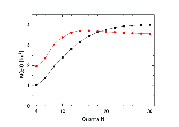
Figure 1: Dependence of the monopole strengths $M_{N}({\rm E0})$ on the model space of the ground state wave function characterized as quanta $N$ [see Eq. (74)]. The square and circle points correspond to $M_{N}({\rm E0};{0^{+}_{1}}\rightarrow{0^{+}_{2}})$ and $M_{N}({\rm E0};{0^{+}_{1}}\rightarrow{0^{+}_{3}})$, respectively.

and study the dependence on $N$ of this quantity. Figure 1 shows the calculated results of $M_{N}({\rm E0},0_{1}^{+}-0_{k}^{+}),(k=2,3)$ as a function $N$. The values of $M_{N}({\rm E0},0_{1}^{+}-0_{k}^{+})$ for $N=4$ are the monopole matrix elements without ground state correlation which we discussed in detail in the above. They are $M_{N=4}({\rm E0},0_{1}^{+}-0_{2}^{+})$ = 1.39 fm² and $M_{N=4}({\rm E0},0_{1}^{+}-0_{3}^{+})$ = 2.36 fm². These values are very close to the values given in Eqs. (71) and (72) for which the normalization constants $N_{k}$ are not accounted. We clearly see that the values of $M_{N}({\rm E0},0_{1}^{+}-0_{k}^{+})$ grow almost monotonously as $N$ becomes larger. At $N$ = 30, the values are already converged, and they are $M_{N=30}({\rm E0},0_{1}^{+}-0_{2}^{+})$ = 4.01 fm² and $M_{N=30}({\rm E0},0_{1}^{+}-0_{3}^{+})$ = 3.56 fm². These converged values are very close to the observed values, and the difference from the observed values is only within 13 %. Thus we have shown that by taking into account the ground state correlation theoretical values are improved as to attain the reproduction of the data within a factor of $1.13$.

An important reason why the ground state correlation enhances the monopole strengths is explained as follows. We study the deviation of the ground-state wave function $|0^{+}_{1}\rangle$ obtained by the ¹²C+$\alpha$ OCM from the doubly closed shell wave function. For this purpose we define a modified doubly closed shell model wave function $\Phi_{0^{+}}(\beta)$ ($\beta$ denoting the size parameter of the ¹²C+$\alpha$ relative wave function) and calculate the squared overlap of it with the OCM ground state wave function $|0^{+}_{1}\rangle$ obtained with the full model space,

$${\Phi_{0^{+}}(\beta)}=N_{g0}(\beta)\frac{1}{\sqrt{{}_{16}C_{4}}}{\cal A}\{[{\cal R}_{40}(\mbox{\boldmath$r$},\beta)\phi_{L=0}({}^{12}{\rm C})]_{J=0}\phi(\alpha)\},$$ (75)

$$P(\beta/(3\nu_{N}))=\left|\langle{\Phi_{0^{+}}(\beta)}|{0^{+}_{1}}\rangle\right|^{2},$$ (76)

where $N_{g0}(\beta)$ is the normalization constant. When $\beta$ is equal to $3\nu_{N}$, the wave function $\Phi_{0^{+}_{1}}(\beta=3\nu_{N})$ is equivalent to the doubly closed shell model wave function in Eq. (6), which originally has the $\alpha$ cluster degree of freedom or sort of like a seed of $\alpha$ clustering, as discussed in Sec. II.1. For $\beta<3\nu_{N}$, ${\Phi_{0^{+}}(\beta)}$ expresses a wave function in which the ¹²C+$\alpha$ relative motion or the seed of $\alpha$ clustering is swollen in comparison with those in the doubly closed shell model wave function. Thus, the study of the dependence of the squared overlap $P$ on the parameter $\beta/(3\nu_{N})$ gives a rough indication on the degree of the deviation from the doubly closed wave function, i.e. the degree of $\alpha$ clustering activated in the ground state. We found that $P$ has the maximum value of 0.958 at $\beta/(3\nu_{N})=0.847$ [vs. $P=0.890$ at $\beta/(3\nu_{N})=1$]. The result of $\beta/(3\nu_{N})=0.847$ means that in the ground state wave function $|0^{+}_{1}\rangle$ the ¹²C+$\alpha$ relative motion or the seed of $\alpha$ clustering is definitely swollen in comparison with those in the doubly closed shell model wave function. Thus the ground state correlation makes the structure of the ground state closer to the ¹²C+$\alpha$ cluster structure in the $0^{+}_{2}$ and $0^{+}_{3}$ states, and then the monopole strengths become significantly larger in comparison with those with no ground state correlation.

III.2 Monopole transition matrix elements in ¹²C

The analytical expression of the monopole transition matrix element $M({\rm E0},0^{+}_{1}-0^{+}_{2})$ is demonstrated in Eq. (64), which depends on the nucleon size parameter $\nu_{N}$ and width parameter of the Hoyle state $\gamma$. The expression of the monopole matrix element consists of three parts like the case of ¹⁶O, and the dominant part is the radial integral referring the relative motions among three $\alpha$ clusters, ${\langle R_{40}(r,\nu_{N})|r^{2}|R_{60}(r,\nu_{N})\rangle}=\sqrt{21/8}/\nu_{N}$. The strength of the radial integral is a few times larger than the single particle monopole strengths, $\langle 0s|r^{2}|1s\rangle$ and $\langle 0p|r^{2}|1p\rangle$.

In the present study we use the value $\nu_{N}=0.168\ {\rm fm}^{-2}$, which reproduces the observed rms radius of ¹²C with the SU(3) shell model wave function in Eqs. (51)$\sim$(53). The monopole matrix element in Eq. (64) which is expressed as $M({\rm E0},0_{2}^{+}-0_{1}^{+})=\xi_{5}\times 0.882/\nu_{N}$ ${\rm fm}^{2}$ contains $\xi_{5}$ which depends on $\gamma$. In Table 2, we display $\xi_{5}$ and $M({\rm E0},0_{2}^{+}-0_{1}^{+})$ calculated at several $\gamma$ values. According to Ref. funaki , we should use the value of $\gamma\approx 0.018$ fm^-2. With this value of $\gamma$, the Bose-condensate wave function has a very large (almost 100 %) overlap with the full solution of the $3\alpha$ RGM for the Hoyle state and gives an rms radius 3.8 fm for the Hoyle state. For $\gamma$ = 0.018 fm^-2, we obtain $\xi_{5}=0.191$, which is relatively small in comparison with $\eta_{6}=0.379$ and $\zeta_{6}=0.570$ in the case of ¹⁶O in Sec. III.1. This leads to

$$M({\rm E0},0_{2}^{+}-0_{1}^{+})=0.19\times\frac{0.882}{\nu_{N}}=1.3{\rm fm}^{2},$$ (77)

which is of the same order of magnitude as the observed value ($5.4\pm 0.2$ ${\rm fm}^{2}$ ajzen86 ) but reproduces only about 25 % in comparison with that. This value of about 25 % is a little bit smaller in contrast to that of the ¹⁶O case (see the previous subsection §III.1) in which our simple estimates are larger than about 40% of the experimental data.

We should note that in more realistic situation the description of the ground state adopted here for ¹²C using the SU(3) shell model is not necessarily good and a deviation from the SU(3) shell model representation should be taken into account supple . According to the structure study of ¹²C with the $3\alpha$ orthogonality condition model (OCM) yamada , the SU(3)$(\lambda,\mu)=(0,4)$ component with the lowest oscillator quantum ($N_{TOT}=8$) is only about 60 % in the ground state. The smallness of the SU(3)$(\lambda,\mu)=(0,4)$ component with the lowest oscillator quantum ($N_{TOT}=8$) is in contrast to the ¹⁶O case, in which the ground state is well described by the doubly closed shell model wave function $(0s)^{4}(0p)^{12}$: The SU(3)$(\lambda,\mu)=(0,0)$ component with the lowest quantum ($N_{TOT}=12$) of the ¹⁶O ground state is as large as about 90% suzuki .

Here we demonstrate the effect of the ground state correlation to the monopole matrix element by adopting the following wave function for the ground state funaki :

$$\Psi_{G}({\widetilde{\gamma}},\nu_{N})={\cal N}_{G}\sqrt{\frac{4!4!4!}{12!}}{\cal A}[\exp\{-{\widetilde{\gamma}}(2\mbox{\boldmath$s$}^{2}+\frac{8}{3}\mbox{\boldmath$t$}^{2})\}\phi(\alpha_{1})\phi(\alpha_{2})\phi(\alpha_{3})],$$ (78)

where ${\cal N}_{G}$ is normalization constant. This wave function is called THSR wave function and depends on two parameters ${\widetilde{\gamma}}$ and $\nu_{N}$. We impose the condition that this wave function reproduces the observed rms radius, 2.47 fm, of the ground state. Then, the ratio ${\widetilde{\gamma}}/\nu_{N}$ is the only parameter which describes the property of the ground state. It is noted that $\Psi_{G}({\widetilde{\gamma}},\nu_{N})$ with ${\widetilde{\gamma}}/\nu_{N}=1$ agrees with the SU(3) $(\lambda,\mu)=(0,4)$ shell model wave function in Eqs. (51)$\sim$(53), demonstrating directly that the wave function originally has sort of like a seed of $3\alpha$ clustering. Taking the ${\widetilde{\gamma}}$ value a little smaller than $\nu_{N}$, $\Psi_{G}({\widetilde{\gamma}},\nu_{N})$ deviates from the SU(3) shell model wave function and the slightly more relaxed spatial clustering of $3\alpha$ clusters than the SU(3) wave function is induced in the ground state, i.e. $\Psi_{G}({\widetilde{\gamma}},\nu_{N})$ expresses sort of like a generalized SU(3) wave function in which the seed of $3\alpha$ clustering are slightly swollen in comparison with the original SU(3) wave function. This is the ground state correlation taking into account here, which is similar to the case in ¹⁶O as discussed in Sec. III.1. In Ref. funaki , it is reported that the ground state wave function of the $3\alpha$ RGM calculation of Refs. kami and uega can be well approximated by this kind of wave function. The amount of the $3\alpha$-like ground state correlation, thus, can be characterized by the ratio ${\widetilde{\gamma}}/\nu_{N}$, which should be less than or equal to unity. In the $3\alpha$ cluster model supple ; funaki ; kami ; uega ; yamada , the nucleon size parameter $\nu_{N}$ is usually chosen to reproduce the rms radius of $\alpha$ cluster, $\nu_{N}=0.275~{}{\rm fm}^{-2}$ which is larger than that for the SU(3) shell model wave function ($\nu_{N}=0.168~{}{\rm fm}^{-2}$) shown above. The estimation of ${\widetilde{\gamma}}/\nu_{N}$ for the ground state wave function given by Ref. funaki is as small as ${\widetilde{\gamma}}/\nu_{N}\sim 0.29$. This small value indicates that the ground state of ¹²C has a significant amount of the $3\alpha$ correlation. Below we change the value of the parameter ${\widetilde{\gamma}}/\nu_{N}$ from $1.0$ down to $0.27$.

The wave function of the Hoyle state is constructed so as to be orthogonal to the ground state wave function $\Psi_{G}$ in Eq. (78) and is given as follows:

$$\Psi_{H}(\gamma,{\widetilde{\gamma}},\nu_{N})={\cal N}_{H}(1-P)\sqrt{\frac{4!4!4!}{12!}}{\cal A}[\exp\{-\gamma(2\mbox{\boldmath$s$}^{2}+\frac{8}{3}\mbox{\boldmath$t$}^{2})\}\phi(\alpha_{1})\phi(\alpha_{2})\phi(\alpha_{3})],$$ (79)

$$P\equiv|\Psi_{G}({\widetilde{\gamma}},\nu_{N})\rangle\langle\Psi_{G}({\widetilde{\gamma}},\nu_{N})|,$$ (80)

where ${\cal N}_{H}$ is normalization constant. The width parameter $\gamma$ is determined so as to reproduce the rms radius of the Hoyle state, 3.8 fm. The Hoyle state of ¹²C ($0^{+}_{2}$) is known to have a dilute $3\alpha$ condensate structure with the nuclear radius of about 4 fm. This exotic structure of the Hoyle state was found to be described simply funaki with a single $\alpha$-condensate wave function given in Eq. (79). The monopole matrix element given as

$${M({\rm E0},0^{+}_{1}-0^{+}_{2}})={\langle\Psi_{G}({\widetilde{\gamma}},\nu_{N})|\frac{1}{2}\sum_{i=1}^{12}(\mbox{\boldmath$r$}_{i}-\mbox{\boldmath$r$}_{G})^{2}|\Psi_{H}(\gamma,{\widetilde{\gamma}},\nu_{N})\rangle},$$ (81)

depending only on the parameter ${\widetilde{\gamma}}/\nu_{N}$.

Table 3 shows the values of the monopole matrix elements [Eq. (81)] calculated at several ${\widetilde{\gamma}}/\nu_{N}$ values. We see that the monopole matrix element increases as the ratio ${\widetilde{\gamma}}/\nu_{N}$ decreases from unity, namely as the $3\alpha$-like correlation becomes stronger in the ground state. This can be reasonably understood from the fact that the ground state wave function $\Psi_{G}$ with stronger $3\alpha$-like correlation has larger $3\alpha$-cluster component which makes larger the overlap with the Hoyle state wave function $\Psi_{H}$ with the dilute $3\alpha$ cluster structure, and then the monopole matrix element becomes larger. At the value of ${\widetilde{\gamma}}/\nu_{N}\sim 0.27$, the monopole matrix element is about $4.0$ fm², which is about three times larger than that for ${\widetilde{\gamma}}/\nu_{N}=1$, and is closer to the observed value $5.4\pm 0.2$ fm². It is noted that ${\widetilde{\gamma}}/\nu_{N}\sim 0.27$ gives the nucleon size parameter $\nu_{N}\sim 0.26~{}{\rm fm}^{-2}$ which corresponds to the value used usually in the microscopic $3\alpha$ cluster model calculations supple ; funaki ; kami ; uega ; yamada . Without the ground state correlation the calculated monopole value is smaller than the observed value by a factor of 4.15 but now with inclusion of the ground state correlation the calculated monopole value changed to be smaller only by a factor of 1.35 than the observed value.

IV Discussions and Summary

The monopole transitions from cluster states to ground states in light nuclei are rather large which is comparable with the single particle strength. The single particle estimate of the monopole transition is based on the assumption that the excited state has a one-particle one-hole excitation from the ground state. However, the cluster structure is very different from the shell-model-like structure of the ground state, and its state is described as a superposition of many-particle many-hole configurations when it is expanded by shell model configurations. This means that in the excited state with a cluster structure, the component of a one-particle one-hole excitation from the ground state configuration is expected to be very small. Therefore the observation of rather large monopole strengths for cluster states which are comparable with single particle strength looks not to be easy to explain. Under this kind of understanding it has been often regarded that the monopole transition occurs through the mixing of shell model wave function $|\rm{shell}\rangle$ and the cluster model wave function $|\rm{cluster}\rangle$

$$|\rm{Ground}\rangle=\alpha|\rm{shell}\rangle+\beta|\rm{cluster}\rangle,$$ (82)

$$|\rm{Excited}\rangle=-\beta|\rm{shell}\rangle+\alpha|\rm{cluster}\rangle.$$ (83)

Since it is assumed that the monopole operator $O_{M}$ does not connect $|\rm{cluster}\rangle$ and $|\rm{shell}\rangle$, $\langle\rm{cluster}|{\it O_{M}}|\rm{shell}\rangle$ = 0, the monopole matrix element is considered to come from the diagonal matrix elements (for example see Ref. bertsch ),

$$\langle\rm{Excited}|{\it O_{M}}|\rm{Ground}\rangle=\alpha\beta(\langle\rm{cluster}|{\it O_{M}}|\rm{cluster}\rangle-\langle\rm{shell}|{\it O_{M}}|\rm{shell}\rangle).$$ (84)

Our explanation of the strong monopole transition between ground state and excited cluster states is quite different from this explanation. We insist that the order of magnitude of the strong monopole transition is given by the matrix element $\langle\rm{cluster}|{\it O_{M}}|\rm{shell}\rangle\neq$ 0,

$$\langle\rm{Excited}|{\it O_{M}}|\rm{Ground}\rangle\approx\langle\rm{cluster}|{\it O_{M}}|\rm{shell}\rangle,\ ({\rm for}\ {\rm order}\ {\rm of}\ {\rm magnitude}).$$ (85)

Our argument is based on the Bayman-Bohr theorem which says that the SU(3) shell-model wave function which describes rather well the structure of the ground state of light nuclei is equivalent in most cases to cluster model wave function. The implication of this theorem is that the clustering degree of freedom is already embedded even in the shell model wave function. In the present study the monopole excitation of the ground state to cluster states is understood as just the excitation of the inter-cluster relative motion in the ground state to the inter-cluster relative motion in excited cluster states. This resembles the monopole excitation of the single nucleon motion. Our understanding was explicitly shown to be true by deriving the analytical expressions of the monopole matrix elements.

In this paper we analyzed the monopole transitions in ¹⁶O between the ground state and ¹²C + $\alpha$ cluster states ($0^{+}_{2}$ and $0^{+}_{3}$) together with the one in ¹²C between the ground state and $3\alpha$ cluster state ($0^{+}_{2}$: Hoyle state). According to the Bayman-Bohr theorem, the doubly closed shell model wave function of ¹⁶O, which has the SU(3)($\lambda\mu$)=(00) symmetry and total quanta $N_{\rm TOT}=12$, is equivalent to the ¹²C ($0^{+}$) + $\alpha$ cluster wave function as well as ¹²C ($2^{+}$) + $\alpha$ with orbital angular momentum of the inter-cluster relative motion $L_{r}=0$ and $2$, respectively. The number of oscillator quanta of the inter-cluster relative motion $N_{r}$ is 4. Similarly, the ground state wave function of ¹²C with SU(3) ($\lambda\mu$) = (04) and $N_{\rm TOT}=8$ is equivalent to the $3\alpha$ cluster wave function. The number of oscillator quanta of the inter-cluster relative motion with respect to each of two Jacobi coordinates is $N_{r}$ = 4. On the other hand, the $0^{+}_{2}$ [$0^{+}_{3}$] state of ¹⁶O has a ¹²C($0^{+}$)+$\alpha$ cluster structure [¹²C($2^{+}$)+$\alpha$] with the relative orbital angular momentum $L_{r}=0$ [$L_{r}=2$]. The $0^{+}_{2}$ state of ¹²C has a $3\alpha$ cluster structure with $S$-wave relative angular momenta referring to two Jacobi coordinates for $3\alpha$ clusters.

The analytical expressions of the monopole matrix elements we derived for the above transitions in ¹⁶O and ¹²C are composed of three factors. The most important factor is the radial integrals with harmonic oscillator wave functions $\langle N_{r}=6,L_{r}|r^{2}|N_{r}=4,L_{r}\rangle$ with $L_{r}=0$ or 2. The values of these integrals are a few times larger than the single particle monopole transition matrix elements in p-shell nuclei, ${\langle 1s|r^{2}|0s\rangle}$ = ${\langle N_{r}=2,L_{r}=0|r^{2}|N_{r}=0,L_{r}=0\rangle}$ and ${\langle 1p|r^{2}|0p\rangle}$ = ${\langle N_{r}=3,L_{r}=1|r^{2}|N_{r}=1,L_{r}=1\rangle}$. The second factor is the amplitude (not squared amplitude) of the $2\hbar\omega$ - excited harmonic oscillator wave function in the cluster states which is denoted as $\eta_{6}$ for $M({\rm E0},0^{+}_{1}-0^{+}_{2})$ and $\zeta_{6}$ for $M({\rm E0},0^{+}_{1}-0^{+}_{3})$ in ¹⁶O and $\xi_{5}$ for $M({\rm E0},0^{+}_{1}-0^{+}_{2})$ in ¹²C. They are not so small; $\eta_{6}$ = 0.38, $\zeta_{6}$ = 0.57, and $\xi_{5}$ = 0.19. The third factor is due to the antisymmetrization among nucleons, which is denoted as $\sqrt{\tau_{0,4}/\tau_{0,6}}$ or $\sqrt{\tau_{2,4}/\tau_{2,6}}$ in ¹⁶O and $\sqrt{\langle F_{4}\rangle/\langle F_{5}\rangle}$ in ¹²C. Since the quantities with strong antisymmetrization effect are contained in the form of ratio, the third factor has magnitude close to unity. As is expected from the analytical expressions, the calculated numerical values of the monopole matrix elements were shown to have the same order of magnitude as the observed values which are comparable with the single nucleon strength.

Although the calculated values of the monopole matrix elements without ground state correlation surely reproduce the order of magnitude of the observed values, when compared with the data in detail, they are a few times smaller than the observed values. In the case of ¹⁶O, two kinds of theoretical values of $M({\rm E0},0^{+}_{1}-0^{+}_{2})$ are 60 % and 38 % of the observed values, respectively, while those of $M({\rm E0},0^{+}_{1}-0^{+}_{3})$ are 96 % and 63 %. In the case of ¹²C, theoretical value of $M({\rm E0},0^{+}_{1}-0^{+}_{2})$ is 25 % of the observed value. Therefore we next investigated the effect of the ground state correlation to the monopole matrix elements. The ground state correlation we considered was the one caused by the activation of the clustering degree of freedom described by Bayman-Bohr theorem. In the calculation of the monopole strength without ground state correlation, we only considered the clustering degree of freedom rather in a static way. Namely we did not consider the dynamical effect of the clustering degree of freedom which excites the ground state configuration toward including higher quantum configurations. We know that the clustering degree of freedom described by Bayman-Bohr theorem has the physical reality because we observe many excited cluster states which are formed by exciting the clustering degree of freedom embedded in the ground state. Therefore taking into account the ground state correlation caused by the clustering degree of freedom described by Bayman-Bohr theorem is very natural and should be studied.

The investigation of the effect of the ground state correlation to the monopole strength in ¹⁶O was made in the framework of the ¹²C + $\alpha$ OCM. It is because, in discussing the monopole strength without ground state correlation in Sec. II, we used the results of the ¹²C + $\alpha$ OCM in Ref. suzuki . We repeated the same calculation as one in Ref. suzuki . We found that 1) increasing the amount of the ground state correlation, the monopole strengths are growing almost monotonously, and 2) at a full amount of the ground state correlation, the monopole strengths are reproduced within a factor of $1.13$ in comparison with the observed values. The reason why the ground state correlation enhances the monopole strengths was discussed with a simple approach. In the case of ¹²C, the investigation of the effect of the ground state correlation to the monopole strength was performed by expressing the ground state with the so-called THSR wave function tohsaki . This wave function has two parameters ${\widetilde{\gamma}}$ and $\nu_{N}$. When ${\widetilde{\gamma}}$ = $\nu_{N}$, the wave function is just equal to the SU(3) wave function with $N_{TOT}=8$ and $(\lambda,\mu)=(0,4)$. As we make the ratio ${\widetilde{\gamma}}/\nu_{N}$ smaller than unity, the wave function contains more amount of the ground state correlation. We found that at a full amount of the ground state correlation, the monopole strength is reproduced within a factor of $1.35$ in comparison with the observed value.

The implication of the Bayman-Bohr theorem has been misunderstood such that the cluster model description is rather unnecessary, since a cluster model wave function is equivalent to a shell model wave function. The existence of cluster states especially as excited states is well established these days. Thus, the implication of the Bayman-Bohr theorem should be understood straightforwardly as follows. If the ground state is well described by an SU(3) shell model wave function equivalent to a cluster model wave function, the ground state possesses two different characters simultaneously, shell-model-state character and cluster-model-state character. This means that the ground state has mean-field degree of freedom and clustering degree of freedom simultaneously. Both of them can be excited, when the nucleus is stimulated by an external field. The monopole excitation to excited cluster states demonstrates us directly the evidence that the clustering degree of freedom is embedded in the ground state. In this paper we showed that the clustering degree of freedom embedded in the ground state can reproduce the order of magnitude of the monopole strength even without taking into account the ground state correlation. Moreover it was demonstrated that, if we take into account the ground state correlation activating the clustering degree of freedom described by the Bayman-Bohr theorem, the monopole strengths are reproduced within a factor of $1.13$ in ¹⁶O and within a factor of $1.35$ in ¹²C, in comparison with the observed values.

Our present study ascertains that the monopole transition between cluster and ground states in light nuclei is generally strong as to be comparable to the single particle strength. The measurement of strong monopole transitions or excitations, therefore, is in general very useful for the study of cluster states.

One of the authors (Y. F.) is grateful for the financial assistance from the Special Postdoctoral Researcher Program of RIKEN.

Appendix A The energy-weighted sum rule of monopole transition by the use of the Jacobi coordinate

We discuss here the energy-weighted sum rule of the monopole transition. The sum rule is written as follows

$$\sum_{k}|\langle k|\frac{1}{2}\sum_{i=1}^{A}(\mbox{\boldmath$r$}_{i}-\mbox{\boldmath$r$}_{G})^{2}|g\rangle|^{2}(E_{k}-E_{g})=\frac{\hbar^{2}}{2m}AR^{2}_{\rm rms},$$ (86)

$$R^{2}_{\rm rms}=\frac{1}{A}\langle g|\sum_{i=1}^{A}(\mbox{\boldmath$r$}_{i}-\mbox{\boldmath$r$}_{G})^{2}|g\rangle,$$ (87)

where $|g\rangle$ and $E_{g}$ stand for the ground state and its energy, respectively, $|k\rangle$ and $E_{k}$ represent the $k$-th excited state and its energy, respectively, and $\mbox{\boldmath$r$}_{G}$ stands for the center-of-mass coordinate.

In ¹⁶O, the observed value of $R_{\rm rms}$ is 2.67 fm and then the energy-weighted sum rule value $(\hbar^{2}/2m)16R^{2}_{\rm rms}$ is 2361 fm${}^{4}\cdot$MeV. In the case of the $0^{+}_{2}$ state at 6.05 MeV which has $M({\rm E0},0^{+}_{1}-0^{+}_{2})_{\rm exp}$ = 3.55 fm², the energy-weighted monopole transition strength is $(3.55)^{2}\times 6.05=76.3$ fm${}^{4}\cdot$MeV. This value is 3.2 % of the energy-weighted sum rule value. In the case of the $0^{+}_{3}$ state at 12.05 MeV which has $M({\rm E0},0^{+}_{1}-0^{+}_{3})_{\rm exp}$ = 4.03 fm², the energy-weighted monopole transition strength is $(4.03)^{2}\times 12.05=196$ fm${}^{4}\cdot$MeV. This value is 8.3 % of the energy-weighted sum rule value. The sum of the energy-weighted monopole transition strengths of $0^{+}_{2}$ and $0^{+}_{3}$ states is 11.5 % of the energy-weighted sum rule value. In ¹²C, the observed value of $R_{\rm rms}$ is 2.37 fm and then the energy-weighted sum rule value $(\hbar^{2}/2m)12R^{2}_{\rm rms}$ is 1395 fm${}^{4}\cdot$MeV. In the case of the $0^{+}_{2}$ state at 7.66 MeV which has $M({\rm E0},0^{+}_{1}-0^{+}_{2})_{\rm exp}$ = 5.4 fm², the energy-weighted monopole transition strength is $(5.4)^{2}\times 7.66=223$ fm${}^{4}\cdot$MeV. This value is 16 % of the energy-weighted sum rule value. These percentage values show that the strength of the monopole transition or excitation to cluster states shares an appreciable portion of the energy-weighted sum rule value.

The formula of the energy-weighted sum rule of monopole transition is obtained by calculating the double commutator of the monopole transition operator $O_{M}$ and the system Hamiltonian $H$

$$[O_{M},[H,O_{M}]],\ \ \ O_{M}=\frac{1}{2}\sum_{i=1}^{A}(\mbox{\boldmath$r$}_{i}-\mbox{\boldmath$r$}_{G})^{2}.$$ (88)

The calculation of the double commutator looks tedious due to the existence of the center-of-mass coordinate $\mbox{\boldmath$r$}_{G}$ but it can be made very easily by using the Jacobi coordinate. For the Hamiltonian $H$ with momentum-independent interaction, $H$ can be replaced by the kinetic energy operator $K$

$$[O_{M},[H,O_{M}]]=[O_{M},[K,O_{M}]],\ \ \ K=\frac{-\hbar^{2}}{2m}\sum_{i=1}^{A}\left(\frac{\partial}{\partial\mbox{\boldmath$r$}_{i}}\right)^{2}-\frac{-\hbar^{2}}{2Am}\left(\frac{\partial}{\partial\mbox{\boldmath$r$}_{G}}\right)^{2}.$$ (89)

Now we introduce the normalized Jacobi coordinates as

$$\mbox{\boldmath$x$}_{j} = \sqrt{\frac{j}{j+1}}\left(\frac{1}{j}\sum_{i=1}^{j}\mbox{\boldmath$r$}_{i}-\mbox{\boldmath$r$}_{j+1}\right),\ \ \ j=1\sim A-1,$$ (90)

$$\mbox{\boldmath$x$}_{A} = \sqrt{\frac{1}{A}}\sum_{i=1}^{A}\mbox{\boldmath$r$}_{i}=\sqrt{A}\mbox{\boldmath$r$}_{G}.$$ (91)

One can easily check that the linear transformation from $\{\mbox{\boldmath$r$}_{i},i=1\sim A\}$ to $\{\mbox{\boldmath$x$}_{j},j=1\sim A\}$ is unitary. Therefore we have

$$\sum_{i=1}^{A}\mbox{\boldmath$r$}_{i}^{2}=\sum_{j=1}^{A}\mbox{\boldmath$x$}_{j}^{2},$$ (92)

$$\sum_{i=1}^{A}(\mbox{\boldmath$r$}_{i}-\mbox{\boldmath$r$}_{G})^{2}=\sum_{i=1}^{A}\mbox{\boldmath$r$}_{i}^{2}-A\mbox{\boldmath$r$}_{G}^{2}=\sum_{j=1}^{A-1}\mbox{\boldmath$x$}_{j}^{2},$$ (93)

$$\sum_{i=1}^{A}\left(\frac{\partial}{\partial\mbox{\boldmath$r$}_{i}}\right)^{2}=\sum_{j=1}^{A}\left(\frac{\partial}{\partial\mbox{\boldmath$x$}_{j}}\right)^{2},$$ (94)

$$\sum_{i=1}^{A}\left(\frac{\partial}{\partial\mbox{\boldmath$r$}_{i}}\right)^{2}-\frac{1}{A}\left(\frac{\partial}{\partial\mbox{\boldmath$r$}_{G}}\right)^{2}=\sum_{j=1}^{A-1}\left(\frac{\partial}{\partial\mbox{\boldmath$x$}_{j}}\right)^{2},$$ (95)

Thus we have

$$O_{M} = \frac{1}{2}\sum_{j=1}^{A-1}\mbox{\boldmath$x$}_{j}^{2},$$ (96)

$$K = \frac{-\hbar^{2}}{2m}\sum_{j=1}^{A-1}\left(\frac{\partial}{\partial\mbox{\boldmath$x$}_{j}}\right)^{2},$$ (97)

When we use the above expressions of $O_{M}$ and $K$ by the normalized Jacobi coordinates, we can easily obtain the following result

$$[O_{M},[H,O_{M}]]=[O_{M},[K,O_{M}]]=\frac{\hbar^{2}}{m}\sum_{j=1}^{A-1}\mbox{\boldmath$x$}_{j}^{2}=\frac{\hbar^{2}}{m}\sum_{i=1}^{A}(\mbox{\boldmath$r$}_{i}-\mbox{\boldmath$r$}_{G})^{2}.$$ (98)

We thus have the formula of the energy-weighted sum rule of monopole transition as follows

$$\frac{\hbar^{2}}{2m}\langle g|\sum_{i=1}^{A}(\mbox{\boldmath$r$}_{i}-\mbox{\boldmath$r$}_{G})^{2}|g\rangle=\frac{1}{2}\langle g|[O_{M},[H,O_{M}]]|g\rangle$$ (99)

$$\ \ =\sum_{k}|\langle k|\frac{1}{2}\sum_{i=1}^{A}(\mbox{\boldmath$r$}_{i}-\mbox{\boldmath$r$}_{G})^{2}|g\rangle|^{2}(E_{k}-E_{g}).$$ (100)

Appendix B Description of ¹⁶O and ¹²C ground states with SU(3) wave function

The total number of the oscillator quanta $N_{TOT}$ possessed by the doubly closed shell wave function of ¹⁶O is $N_{TOT}=12$. For $N_{TOT}=12$, it is possible to construct many ¹²C+$\alpha$ cluster wave functions with various SU(3) symmetry $(\lambda,\mu)$, ${\cal A}\{[{\cal R}_{4}(\mbox{\boldmath$r$})\phi({}^{12}{\rm C})]_{(\lambda,\mu)}\phi(\alpha)\}$. These wave functions, however, become all zero except for $(\lambda,\mu)=(0,0)$, because of the nature of the doubly closed wave function. Using the following relation

$$[{\cal R}_{4L}(\mbox{\boldmath$r$})\phi_{L}({}^{12}{\rm C})]_{J=0}=\sum_{(\lambda,\mu)}\langle(4,0)L,(0,4)L||(\lambda,\mu)0\rangle[{\cal R}_{4}(\mbox{\boldmath$r$})\phi({}^{12}{\rm C})]_{(\lambda,\mu)},$$ (101)

we have

$${\cal A}\{[{\cal R}_{4L}(\mbox{\boldmath$r$})\phi_{L}({}^{12}{\rm C})]_{J=0}\phi(\alpha)\}$$

$$\hskip 42.67912pt=\sum_{(\lambda,\mu)}\langle(4,0)L,(0,4)L||(\lambda,\mu)0\rangle{\cal A}\{[{\cal R}_{4}(\mbox{\boldmath$r$})\phi({}^{12}{\rm C})]_{(\lambda,\mu)}\phi(\alpha)\}$$

$$\hskip 42.67912pt=\langle(4,0)L,(0,4)L||(0,0)0\rangle{\cal A}\{[{\cal R}_{4}(\mbox{\boldmath$r$})\phi({}^{12}{\rm C})]_{(\lambda,\mu)=(0,0)}\phi(\alpha)\},$$ (102)

for $L=0$, 2, and 4. This relation is an explanation of the equalities of Eqs. (6)$\sim$(8).

Similar argument holds for the ground state of ¹²C. Although there can be constructed many 3$\alpha$ cluster wave functions with various SU(3) symmetry $(\lambda,\mu)$, ${\cal A}\{[{\cal R}_{N_{1}}(\mbox{\boldmath$s$},2\nu_{N}){\cal R}_{N_{2}}(\mbox{\boldmath$t$},(8/3)\nu_{N})]_{(\lambda,\mu)}\phi(\alpha_{1})\phi(\alpha_{2})\phi(\alpha_{3})\}$ for $N_{TOT}=N_{1}+N_{2}=8$ which is the lowest number of the total oscillator quanta for ¹²C, only one wave function with $(\lambda,\mu)=(0,4)$ is non-vanishing which is possible for $N_{1}=N_{2}=4$ hori ; kato . Therefore we have the following relations

$${\cal A}\{[{\cal R}_{N_{1}L}(\mbox{\boldmath$s$},2\nu_{N}){\cal R}_{N_{2}L}(\mbox{\boldmath$t$},(8/3)\nu_{N})]_{J=0}\phi(\alpha_{1})\phi(\alpha_{2})\phi(\alpha_{3})\}$$

$$\hskip 11.38092pt=\delta_{N_{1},4}\delta_{N_{2},4}\langle(4,0)L,(4,0)L||(0,4)0\rangle$$

$$\hskip 11.38092pt\times{\cal A}\{[{\cal R}_{N_{1}}(\mbox{\boldmath$s$},2\nu_{N}){\cal R}_{N_{2}}(\mbox{\boldmath$t$},(8/3)\nu_{N})]_{(\lambda,\mu)=(0,4)}\phi(\alpha_{1})\phi(\alpha_{2})\phi(\alpha_{3})\},$$ (103)

for $L=0$, 2, and 4. This relation is an explanation of the equalities of Eqs. (51)$\sim$(53).

Appendix C Dependence of $M({\rm E0},0^{+}_{1}-0^{+}_{2})$ on the width parameter $\gamma$ of the 3$\alpha$ condensed wave function

First we note

$${\cal A}\{{\widehat{\chi}}_{H}(\mbox{\boldmath$s$},\mbox{\boldmath$t$})\phi(\alpha_{1})\phi(\alpha_{2})\phi(\alpha_{3})\}={\cal A}\{{\widehat{\chi}}_{HG}(\mbox{\boldmath$s$},\mbox{\boldmath$t$})\phi(\alpha_{1})\phi(\alpha_{2})\phi(\alpha_{3})\}$$

$$\hskip 28.45274pt-\langle{\cal R}^{8,J=0}_{4,4,L=0}(\mbox{\boldmath$s$},\mbox{\boldmath$t$})|{\widehat{\chi}}_{HG}(\mbox{\boldmath$s$},\mbox{\boldmath$t$})\rangle{\cal A}\{{\cal R}^{8,J=0}_{4,4,L=0}(\mbox{\boldmath$s$},\mbox{\boldmath$t$})\phi(\alpha_{1})\phi(\alpha_{2})\phi(\alpha_{3})\}.$$ (104)

Then we obtain

$$\langle{\widehat{\chi}}_{H}\rangle=\langle{\widehat{\chi}}_{HG}\rangle-\left(\langle{\cal R}^{8,J=0}_{4,4,L=0}(\mbox{\boldmath$s$},\mbox{\boldmath$t$})|{\widehat{\chi}}_{HG}(\mbox{\boldmath$s$},\mbox{\boldmath$t$})\rangle\right)^{2}\langle{\cal R}^{8,J=0}_{4,4,L=0}\rangle,$$ (105)

with the notation

$$\langle G\rangle=\langle G(\mbox{\boldmath$s$},\mbox{\boldmath$t$})\phi(\alpha_{1})\phi(\alpha_{2})\phi(\alpha_{3})|{\cal A}\{G(\mbox{\boldmath$s$},\mbox{\boldmath$t$})\phi(\alpha_{1})\phi(\alpha_{2})\phi(\alpha_{3})\}\rangle.$$ (106)

Next we note

$${\cal A}\{{\widehat{\chi}}_{HG}(\mbox{\boldmath$s$},\mbox{\boldmath$t$})\phi(\alpha_{1})\phi(\alpha_{2})\phi(\alpha_{3})\}=\sum_{n\geq 4}^{\infty}\sum_{n_{1}+n_{2}=n}\langle{\cal R}^{2n,J=0}_{2n_{1},2n_{2},0}(\mbox{\boldmath$s$},\mbox{\boldmath$t$})|{\widehat{\chi}}_{HG}(\mbox{\boldmath$s$},\mbox{\boldmath$t$})\rangle$$

$$\hskip 113.81102pt\times{\cal A}\{{\cal R}^{2n,J=0}_{2n_{1},2n_{2},0}(\mbox{\boldmath$s$},\mbox{\boldmath$t$})\phi(\alpha_{1})\phi(\alpha_{2})\phi(\alpha_{3})\}$$ (107)

$$\hskip 14.22636pt=\left(\frac{2\sqrt{\nu_{N}\gamma}}{\nu_{N}+\gamma}\right)^{3}\sum_{n=4}^{\infty}\left(\frac{\nu_{N}-\gamma}{\nu_{N}+\gamma}\right)^{n}{\cal A}\{F_{n}(\mbox{\boldmath$s$},\mbox{\boldmath$t$})\phi(\alpha_{1})\phi(\alpha_{2})\phi(\alpha_{3})\},$$ (108)

$$F_{n}(\mbox{\boldmath$s$},\mbox{\boldmath$t$})=\sum_{n_{1}+n_{2}=n}\sqrt{\frac{(2n_{1}+1)!!(2n_{2}+1)!!}{(2n_{1})!!(2n_{2})!!}}{\cal R}^{2n,J=0}_{2n_{1},2n_{2},0}(\mbox{\boldmath$s$},\mbox{\boldmath$t$}),$$ (109)

where the following formula is used

$$\langle R_{2n,0}(r,\beta)|\sqrt{4\pi}\left(\frac{2\beta^{\prime}}{\pi}\right)^{\frac{3}{4}}e^{-\beta^{\prime}r^{2}}\rangle=\sqrt{\frac{(2n+1)!!}{(2n)!!}}\left(\frac{2\sqrt{\beta\beta^{\prime}}}{\beta+\beta^{\prime}}\right)^{\frac{3}{2}}\left(\frac{\beta-\beta^{\prime}}{\beta+\beta^{\prime}}\right)^{n},$$ (110)

From Eqs. (106) and (108) we obtain

$$\langle{\widehat{\chi}}_{HG}\rangle=\left(\frac{2\sqrt{\nu_{N}\gamma}}{\nu_{N}+\gamma}\right)^{6}\sum_{n=4}^{\infty}\left(\frac{\nu_{N}-\gamma}{\nu_{N}+\gamma}\right)^{2n}\langle F_{n}\rangle.$$ (111)

By noticing

$$\langle{\cal R}^{8,J=0}_{4,4,0}(\mbox{\boldmath$s$},\mbox{\boldmath$t$})|{\widehat{\chi}}_{HG}(\mbox{\boldmath$s$},\mbox{\boldmath$t$})\rangle=\frac{5!!}{4!!}\left(\frac{2\sqrt{\nu_{N}\gamma}}{\nu_{N}+\gamma}\right)^{3}\left(\frac{\nu_{N}-\gamma}{\nu_{N}+\gamma}\right)^{4},$$ (112)

$$\langle F_{4}\rangle=\left(\frac{5!!}{4!!}\right)^{2}\langle{\cal R}^{8,J=0}_{4,4,0}\rangle\equiv\left(\frac{5!!}{4!!}\right)^{2}\frac{1}{(\widehat{N}_{g0})^{2}},$$ (113)

we obtain

$$\langle{\widehat{\chi}}_{H}\rangle=\left(\frac{2\sqrt{\nu_{N}\gamma}}{\nu_{N}+\gamma}\right)^{6}\sum_{n=5}^{\infty}\left(\frac{\nu_{N}-\gamma}{\nu_{N}+\gamma}\right)^{2n}\langle F_{n}\rangle\equiv\frac{1}{(\widehat{N}_{H})^{2}},$$ (114)

$$D_{H,2n_{1},2n_{2}}\equiv\sqrt{\frac{(2n_{1}+1)!!(2n_{2}+1)!!}{(2n_{1})!!(2n_{2})!!}}\left(\frac{2\sqrt{\nu_{N}\gamma}}{\nu_{N}+\gamma}\right)^{3}\left(\frac{\nu_{N}-\gamma}{\nu_{N}+\gamma}\right)^{n_{1}+n_{2}},$$ (115)

By combining all these formulas we have

$$M({\rm E0},0_{2}^{+}-0_{1}^{+})=\frac{1}{2}\frac{{\widehat{N}}_{H}}{{\widehat{N}}_{g0}}(D_{H,6,4}+D_{H,4,6})\langle R_{40}(r,\nu_{N})|r^{2}|R_{60}(r,\nu_{N})\rangle$$ (116)

$$\hskip 14.22636pt=\frac{1}{2}\sqrt{\frac{\langle{\cal R}^{8,J=0}_{4,4,0}\rangle}{\displaystyle{\left(\frac{2\sqrt{\nu_{N}\gamma}}{\nu_{N}+\gamma}\right)^{6}}\sum_{n=5}^{\infty}\displaystyle{\left(\frac{\nu_{N}-\gamma}{\nu_{N}+\gamma}\right)^{2n}}\langle F_{n}\rangle}}$$

$$\hskip 28.45274pt\times 2\sqrt{\frac{5!!7!!}{4!!6!!}}\left(\frac{2\sqrt{\nu_{N}\gamma}}{\nu_{N}+\gamma}\right)^{3}\left(\frac{\nu_{N}-\gamma}{\nu_{N}+\gamma}\right)^{5}\langle R_{40}(r,\nu_{N})|r^{2}|R_{60}(r,\nu_{N})\rangle$$ (117)

$$\hskip 14.22636pt=\sqrt{\frac{7}{6}}\sqrt{\frac{\langle F_{4}\rangle}{\langle F_{5}\rangle}}\xi_{5}\langle R_{40}(r,\nu_{N})|r^{2}|R_{60}(r,\nu_{N})\rangle,$$ (118)

$$\xi_{5}\equiv\sqrt{\frac{\langle F_{5}\rangle}{\langle F_{5}\rangle+\sum_{n=6}^{\infty}\displaystyle{\left(\frac{\nu_{N}-\gamma}{\nu_{N}+\gamma}\right)^{2(n-5)}}\langle F_{n}\rangle}}.$$ (119)

Appendix D Estimation of $\eta_{N}$ and $\zeta_{N}$ by Ref. suzuki

In Ref. suzuki the ¹⁶O states are expressed by microscopic ¹²C + $\alpha$ cluster wave functions where ¹²C cluster can be excited to its first $2^{+}$ and $4^{+}$ states. This coupled channel problem is solved by using the coupled channel OCM (orthogonality condition model). The wave functions $\Phi$ are expressed by the SU(3)-coupled basis of the ¹²C + $\alpha$ cluster model space, which is in the case of $J=0$

$$\Phi=\sum_{Nq}\xi_{Nq}\Phi_{Nq},$$ (120)

$$\Phi_{N,q=(\lambda,\mu)}=N_{Nq}\frac{1}{\sqrt{\mu_{Nq}}}\frac{1}{\sqrt{{}_{16}C_{4}}}{\cal A}\{[{\cal R}_{N}(\mbox{\boldmath$r$},3\nu_{N})\phi({}^{12}{\rm C})]_{(\lambda,\mu)}\phi(\alpha)\},$$ (121)

$$\mu_{N,q=(\lambda,\mu)}=\langle[{\cal R}_{N}(\mbox{\boldmath$r$},3\nu_{N})\phi({}^{12}{\rm C})]_{(\lambda,\mu)}\phi(\alpha)|{\cal A}\{[{\cal R}_{N}(\mbox{\boldmath$r$},3\nu_{N})\phi({}^{12}{\rm C})]_{(\lambda,\mu)}\phi(\alpha)\}\rangle.$$ (122)

The SU(3)-coupled basis wave functions $\Phi_{N,q=(\lambda,\mu)}$ are ortho-normalized and are the eigenfunctions of normalization kernel with eigenvalues $\mu_{N,q=(\lambda,\mu)}$. The values of the expansion coefficients $\xi_{Nq}$ are given in Table I of the second paper of Ref. suzuki .

Since the wave function of the $0_{2}^{+}$ state shows predominantly a ¹²C($0^{+}$) + $\alpha$ structure, we approximated in this paper the wave function of the $0_{2}^{+}$ state by a pure ¹²C($0^{+}$) + $\alpha$ structure

$$\Phi(0^{+}_{2}) = \sum_{N\geq 6}\eta_{N}\Phi_{N},$$ (123)

$$\Phi_{N} = \frac{1}{\sqrt{\tau_{0,N}}}\frac{1}{\sqrt{{}_{16}C_{4}}}{\cal A}\{R_{N0}(r)Y_{00}(\mbox{\boldmath$\hat{r}$})\phi_{L=0}({}^{12}{\rm C})\phi(\alpha)\}.$$ (124)

This means we adopted the following approximation for each $N$

$$\sum_{q}\xi_{Nq}\Phi_{Nq}\approx\eta_{N}\Phi_{N}.$$ (125)

Therefore we have

$$\eta_{N}\approx\sqrt{\sum_{q}(\xi_{Nq})^{2}}.$$ (126)

The values $\sum_{q}(\xi_{Nq})^{2}$ are tabulated in Table I of the first paper of Ref. suzuki . For $N=6$, we have $\eta_{6}\approx\sqrt{0.144}=0.379$.

From Table I of the second paper of Ref. suzuki , we have in the case of $N=6$ for $0_{2}^{+}$

$$\sum_{q}\xi_{6q}\Phi_{6q}=0.338\Phi_{6,(4,2)}+0.171\Phi_{6,(2,0)}.\ \ ({\rm for}\ 0_{2}^{+})$$ (127)

We should note here that $\Phi_{6,(2,0)}$ is nothing but $\Phi_{(2,0)}^{cl}$ which absorbs the total monopole strength of $\Phi_{CS}$ within the ¹²C + $\alpha$ cluster model space. On the other hand, there holds

$$\Phi_{6}=0.750\Phi_{6,(4,2)}+0.661\Phi_{6,(2,0)}.$$ (128)

This relation is easily obtained by comparing $\langle\Phi_{6}|O_{M}|\Phi_{CS}\rangle$ with $\langle\Phi_{6,(2,0)}|O_{M}|\Phi_{CS}\rangle$:

$$\langle\Phi_{6}|O_{M}|\Phi_{CS}\rangle=\frac{1}{2}\sqrt{\frac{\tau_{0,4}}{\tau_{0,6}}}\langle R_{40}(r,\nu_{N})|r^{2}|R_{60}(r,\nu_{N})\rangle=\frac{0.784}{\nu_{N}},$$ (129)

$$\langle\Phi_{6,(2,0)}|O_{M}|\Phi_{CS}\rangle=\frac{1.19}{\nu_{N}}.$$ (130)

Since the monopole operator $O_{M}$ does not connect $\Phi_{CS}$ with $\Phi_{6,(4,2)}$, we have

$$\langle\Phi_{6,(2,0)}|\Phi_{6}\rangle=\frac{0.784}{1.19}=0.661.$$ (131)

By using $\eta_{6}=0.379$ we have

$$\eta_{6}\Phi_{6}=0.284\Phi_{6,(4,2)}+0.250\Phi_{6,(2,0)}.$$ (132)

The comparison of Eq. (127) with Eq. (132) tells us that the approximation of $\sum_{q}\xi_{6q}\Phi_{6q}$ with $\eta_{6}\Phi_{6}$ is not very good and that the monopole strength of $\sum_{q}\xi_{6q}\Phi_{6q}$ is weaker than that of $\eta_{6}\Phi_{6}$.

The arguments for the $0_{3}^{+}$ state can be made completely in the same way as the $0_{2}^{+}$ state. We obtain following relations

$$\zeta_{6}\approx\sqrt{0.325}=0.570,$$ (133)

$$\sum_{q}\xi_{6q}\Phi_{6q}=0.471\Phi_{6,(4,2)}+0.321\Phi_{6,(2,0)},\ \ ({\rm for}\ 0_{3}^{+}),$$ (134)

$$\Psi_{6}=0.493\Phi_{6,(4,2)}+0.870\Phi_{6,(2,0)},$$ (135)

$$\zeta_{6}\Psi_{6}=0.281\Phi_{6,(4,2)}+0.496\Phi_{6,(2,0)}.$$ (136)

The approximation of $\sum_{q}\xi_{6q}\Phi_{6q}$ with $\zeta_{6}\Psi_{6}$ is not also so good and the monopole strength of $\sum_{q}\xi_{6q}\Phi_{6q}$ is also weaker than that of $\zeta_{6}\Psi_{6}$.

Table 1: Values of $\tau_{0,N}$, $\tau_{2,N}$ and $\tau_{4,N}$ which are calculated with the analytical expression given in Refs. suzuki ; horic .

$N$	$\tau_{0,N}$	$\tau_{2,N}$	$\tau_{4,N}$
4	0.2963	1.4815	2.6667
6	0.3160	0.7831	1.0243
8	0.5615	0.7743	0.8773
10	0.7405	0.8551	0.8985
12	0.8564	0.9182	0.9374
14	0.9247	0.9567	0.9654
16	0.9619	0.9780	0.9818
18	0.9811	0.9890	0.9907
20	0.9908	0.9946	0.9953
22	0.9955	0.9974	0.9977
24	0.9979	0.9987	0.9989

Table 2: $\xi_{5}$ and monopole matrix element $M({\rm E0},0_{2}^{+}-0_{1}^{+})$ in ¹²C calculated at several values of $\gamma$. $M({\rm E0},0_{2}^{+}-0_{1}^{+})$ is given as $\xi_{5}\times 0.882/\nu_{N}$ ${\rm fm}^{2}$, where the value $\nu_{N}=0.168$ ${\rm fm}^{-2}$ is used. $R_{\rm rms}(0_{2}^{+})$ is the corresponding rms radius of the Hoyle state to the adopted values of $\nu_{N}$ and $\gamma$.

$\gamma$ $[{\rm fm}^{-2}]$	$\xi_{5}$	$M({\rm E0},0_{2}^{+}-0_{1}^{+})$ $[{\rm fm}^{2}]$	$R_{\rm rms}(0_{2}^{+})$ [fm]
$0.0238$	$0.338$	$1.775$	$3.56$
$0.0182$	$0.252$	$1.326$	$3.79$
$0.0143$	$0.191$	$1.004$	$4.03$
$0.0115$	$0.147$	$0.773$	$4.28$

Table 3: Dependence of the monopole matrix element in ¹²C on the amount of $3\alpha$-like correlation involved in the ground state, which is characterized by ${\widetilde{\gamma}}/\nu_{N}$. The monopole matrix element is given as $M({\rm E0},0_{2}^{+}-0_{1}^{+})$=$\langle\Psi_{G}({\widetilde{\gamma}},\nu_{N})|\sum_{i=1}^{12}(\mbox{\boldmath$r$}_{i}-\mbox{\boldmath$r$}_{G})^{2}/2|\Psi_{H}(\gamma,{\widetilde{\gamma}},\nu_{N})\rangle$, where $\Psi_{G}({\widetilde{\gamma}},\nu_{N})$ and $\Psi_{H}(\gamma,{\widetilde{\gamma}},\nu_{N})$ are the ground state and Hoyle state wave functions, respectively. The rms radius of the ground-state wave function $\Psi_{G}({\widetilde{\gamma}},\nu_{N})$ is fixed to the experimental one ($2.47$ fm). Then, the ratio ${\widetilde{\gamma}}/\nu_{N}$ is only the parameter to describe the property of the ground state. For a given value of ${\widetilde{\gamma}}/\nu_{N}$, the value of $\gamma$ in $\Psi_{H}(\gamma,{\widetilde{\gamma}},\nu_{N})$ is chosen so as to reproduce the rms radius of the Hoyle state ($3.8$ fm). See the text for details.

${\widetilde{\gamma}}/\nu_{N}$	$M({\rm E0},0_{2}^{+}-0_{1}^{+})$ $[{\rm fm}^{2}]$
$1.000$	$1.326$
$0.705$	$1.810$
$0.498$	$2.473$
$0.309$	$3.597$
$0.274$	$4.035$

References

- (1) Y. Fujiwara, H. Horiuchi, K. Ikeda, M. Kamimura, K. Kato, Y. Suzuki, and E. Uegaki, Prog. Theor. Phys. Supple. 68, 29 (1980).
- (2) H. Horiuchi and K. Ikeda, Prog. Theor. Phys. 40, 277 (1968).
- (3) Y. Suzuki, Prog. Theor. Phys. 55, 1751 (1976); Prog. Theor. Phys. 56, 111 (1976).
- (4) P. Ajzenberg-Selove, Nucl. Phys. A 460, (1986) 1.
- (5) F. Hoyle, Astrophys. J. Supple. 1, 121 (1954).
- (6) T. Kawabata, H. Akimune, H. Fujita, Y. Fujita, M. Fujiwara, K. Hara, K. Hatanaka, M. Itoh, Y. Kanada-En’yo, S. Kishi, K. Nakanishi, H. Sakaguchi, Y. Simbara, A. Tamii, S. Terashima, M. Uchida, T. Wakasa, Y. Yoshida, H. P. Yoshida, M. Yosoi, Phys. Lett. B 646, (2007) 6.
- (7) T. Yamada and Y. Funaki, to be prepared.
- (8) M. Kamimura, Nucl. Phys. A 351, 456 (1981).
- (9) E. Uegaki, S. Okabe, Y. Abe, and H. Tanaka, Prog. Theor. Phys. 57, 1262 (1977) ; E. Uegaki, Y. Abe, S. Okabe, and H. Tanaka, Prog. Theor. Phys. 59, 1031 (1978) ; 62, 1621 (1979).
- (10) B. F. Bayman and A. Bohr, Nucl. Phys. 9, 596 (1958/59).
- (11) J. P. Elliott, Proc. Roy. Soc. (London) A245, 128; 562.
- (12) K. Wildermuth and Th. Kanellopoulos, Nucl. Phys. A 7, 150 (1958); 9, 449 (1958/59).
- (13) K. T. Hecht, Phys. Rev. C16, 2401 (1977).
- (14) A. Tohsaki, H. Horiuchi, P. Schuck, and G. Röpke, Phys. Rev. Lett. 87, 192501 (2001).
- (15) Y. Funaki, A. Tohsaki, H. Horiuchi, P. Schuck, and G. Röpke, Phys. Rev. C 67, 051306(R) (2003).
- (16) H. Horiuchi, Prog. Theor. Phys. 51, 745 (1974).
- (17) H. Horiuchi, Prog.Theor. Phys. 51, 1266 (1974).
- (18) T. Yamada and P. Schuck, Eur. Phys. J. A 26, 185 (2005).
- (19) G. F. Bertsch, Phys. Lett. 21, 70 (1966).
- (20) K. Kato and H. Bando, Prog. Theor. Phys. 53, 692 (1975).