Is there model-independent evidence of the two-photon-exchange effect in the electron-proton elastic scattering cross section?

Abstract

We re-analyze the data of the elastic electron proton scattering to look for model-independent evidence of the two-photon-exchange (TPE) effect. In contrast to previous analyses, TPE effect is parametrized in forms which are free of kinematical-singularity, in addition to being consistent with the constraint derived from crossing symmetry and the charge conjugation. Moreover, we fix the value of $R=G_{E}/G_{M}$ as determined from the data of the polarization transfer experiment. We find that, at high $Q^{2}\geq 2\,GeV^{2}$ values, the contribution of the TPE effect to the slope of $\sigma_{R}$ vs. $\varepsilon$ is large and comparable with that arising from $G_{E}$. It also behaves quasi-linearly in the region of current data, namely, in the range of $0.2<\varepsilon<0.95$. Hence the fact that the current elastic $ep$ cross section data shows little nonlinearity with respect to $\varepsilon$ can not be used to exclude the presence of the TPE effect. More precise data at extreme angles will be crucial for a model-independent extraction of the TPE effect.

PACS: 13.40.GP, 25.30.-c, 25.30.Bf, 24.70.+s, 13.60.Fz

The electric and magnetic form factors $G_{E}$ and $G_{M}$ of the nucleon contain essential piece of our knowledge of the nucleon structure. Traditionally, Rosenbluth method is used to extract $G_{E}$ and $G_{M}$ of the proton from the differential cross section of the electron-proton ($ep$) scattering. Within the one-photon-exchange (OPE) approximation, one has

$$\sigma_{R}(Q^{2},\varepsilon)\equiv\frac{d\sigma}{d\Omega_{Lab}}\frac{\varepsilon(1+\tau)}{\tau\sigma_{Mott}}=G_{M}^{2}(Q^{2})+\frac{\varepsilon}{\tau}G_{E}^{2}(Q^{2}),$$ (1)

where $\tau=Q^{2}/4M_{p}^{2}$ and $1/\varepsilon\equiv 1+2(1+\tau)\tan^{2}\theta_{Lab}/2$, with $\theta_{Lab}$ the laboratory scattering angle such that $0\leq\varepsilon\leq 1$. $\sigma_{Mott}$ is the Mott cross section. At a fixed value of $Q^{2}$, the slope and the intercept of $\sigma_{R}(\varepsilon)\,vs.\,\varepsilon$ is directly related to $G_{E}$ and $G_{M}$, respectively. Through this method it is determined that

$$\mu_{p}R=\mu_{p}G_{E}(Q^{2})/G_{M}(Q^{2})\approx 1,$$ (2)

where $\mu_{p}=2.79$ is the proton anomalous magnetic moment.

Another way to extract the ratio $R=G_{E}/G_{M}$ is to measure the polarizations of the recoil proton in the elastic $ep$ scattering. Within the OPE approximation, the values of $R$ can be extracted according to the following formula [1]:

$$R=-\sqrt{\frac{\tau(1+\varepsilon)}{2\varepsilon}}\cdot\frac{P_{t}}{P_{l}},$$ (3)

where $P_{l}$ and $P_{t}$ are the polarizations, parallel and perpendicular to the proton momentum in the scattering plane, respectively. This method has several advantages over the traditional Rosenbluth separation method. The reason is that the ratio of the two simultaneously measured polarization components greatly reduces systematic uncertainties. For instance, a detailed knowledge of the spectrometer acceptance which plagues the cross section measurements is not required here. Furthermore, the detailed knowledge of the beam polarization and the the polarimeter analyzing power are also not needed because both quantities cancel in measuring the ratio of the form factors. Therefore this method has been considered to be more reliable.

Recent polarization transfer experiments at Jefferson Lab [2, 3] give, however,

$$\mu_{p}R=\mu_{p}G_{E}(Q^{2})/G_{M}(Q^{2})=1-0.13(Q^{2}~{}[\mbox{GeV}^{2}]-0.04),$$ (4)

which differs substantially from the Rosenbluth results of Eq. (2) at high $Q^{2}$. It was suspected that there is a systematic uncertainty common to all Rosenbluth data. However, recent measurements of high $Q^{2}$ $ep$ elastic cross section at the Jefferson Laboratory (JLab) [4, 5] confirmed the earlier Rosenbluth measurements from SLAC [6, 7] in the same $Q^{2}$ region.

It has been proposed [8, 9, 10] that this mismatch can be explained by the two-photon-exchange (TPE) effect not fully accounted for in the standard radiative corrections procedure of Mo and Tsai [11]. So far the only observation of possible TPE effect is in the asymmetry of scattering of transversely polarized electrons from protons. This observable should vanish within the OPE approximation but both SAMPLE experiment at Bates [12] and PVA4 Collaboration at Mainz [13] have observed small but non-zero results. This observable is related to the imaginary part of two-photon exchange amplitude. On the other hand, the unpolarized cross section depends only on the real part of the two-photon exchange amplitude which does not, in general, vanish. It is hence reasonable to expect that the TPE effect would contribute to $\sigma_{R}$. The crucial question is whether this effect is large enough to explain the discrepancy between the results of the Rosenbluth and the polarization transfer methods for the ratio $R$.

To be more specific, let us take a closer look on how the TPE effect would modify the Rosenbluth formula. Including the TPE effect, Eq. (1) is rewritten in the following general form [8]:

$$\sigma_{R}(Q^{2},\varepsilon)=G_{M}^{2}(Q^{2})+\frac{\varepsilon}{\tau}G_{E}^{2}(Q^{2})+F(Q^{2},\varepsilon),$$ (5)

where $F(Q^{2},\varepsilon)$ is a real function describing the effect of the $1\gamma\otimes 2\gamma$ interference. Although the magnitude of $F$ is suppressed by $\alpha_{em}=1/137$ compared to the OPE effect, the $\varepsilon$ dependence of $F(Q^{2},\varepsilon)$ is not necessarily small in comparison with $\varepsilon G_{E}^{2}/\tau$, particularly at higher $Q^{2}$ region where $G_{E}$ and $1/\tau$ are both small. Hence the slope of the $\sigma_{R}(\varepsilon)$ is no longer just $G_{E}^{2}/\tau$ but also includes the linear part of the TPE effect. As a result, the validity of Eq. (1) becomes questionable and the extraction of $G_{E}$ and $G_{M}$ from $\sigma_{R}(\varepsilon)$ needs more sophisticated consideration and the values of $R=G_{E}/G_{M}$ obtained via the Rosenbluth method should also be modified.

There are currently two ways to study the TPE effect in $\sigma_{R}$. The first one is to estimate $F(Q^{2},\varepsilon)$ by calculating the two-photon-exchange $ep$ scattering amplitude with some simple hadronic or partonic models [9, 10, 14]. However, so far there is no complete calculation which is valid at all kinematics. The second way is to analyze the experimental data to search for the nonlinearity in $\sigma_{R}$ with respect to $\varepsilon$ which is regarded as the evidence of the TPE effect [15, 16] since $F(Q^{2},\varepsilon)$ is, in general, not a linear function of $\varepsilon$.

All current model calculations [9, 10, 14] show that the existing discrepancy between the Rosenbluth and the polarization transfer methods can at least be partially explained by the TPE effect [8, 10]. However, several groups [15, 16] have claimed that they cannot find any conclusive evidence for the the nonlinearity of $\sigma_{R}(\varepsilon)$ in their data analyses. The analysis of Ref. [16] set tight limits on the size of the nonlinearity of $\sigma_{R}(\varepsilon)$. Nevertheless, these limits are still consistent with the predictions of the model calculations. In fact, this issue was already discussed in [8]. It was speculated that there may be a simple explanation of the fact the Rosenbluth plot looks linear even if it is strongly affected by the TPE effect. Namely, even if the TPE effect in the cross section is not a linear function of $\varepsilon$, it is still possible for $F$ to behave quasi-linearly within the present experimental uncertainty in the current data region ($0.2<\varepsilon<0.95$). If this is the case, both of the success of Rosenbluth separation in the past and the newly discovered discrepancy can be explained because the $\sigma_{R}(\varepsilon)$ in the certain range of $\varepsilon$ could look like a straight line with its slope a sum of the OPE and TPE effects.

To explore this possibility, one needs to look for some appropriate parametrization of the TPE effect to account for the data of the cross section of the elastic $ep$ scattering. Such a parametrization has to possess general characteristics of the TPE mechanism, as derived from charge conjugation and crossing symmetry in Ref. [17]. Namely, the last term $F$ in Eq. (5) which corresponds to the $1\gamma\otimes 2\gamma$ interference effects should, at a fixed value of $Q^{2}$, satisfy the following constraint

$$F(Q^{2},y)=-F(Q^{2},-y),$$ (6)

where $y=\sqrt{\displaystyle\frac{1-\varepsilon}{1+\varepsilon}}$. In [15], $F(Q^{2},\varepsilon)$ is assumed to take the form

$$F(Q^{2},\varepsilon)\sim\frac{\varepsilon}{y}\mbox{ or }\frac{1}{y}.$$ (7)

However, it suffers from the problem that $1/y$ diverges when $y$ approaches zero, i.e., $\theta_{Lab}\rightarrow 0$, and is hence not acceptable.

In this letter, we study the TPE effect in $\sigma_{R}(\varepsilon)$ directly through data analysis. We choose the data from [7] in order to avoid complication due to different normalizations of different experiments. According to the general argument of  [8], $R=G_{E}/G_{M}$ determined in the polarization transfer method is little affected by the TPE effect, at least in the range of $Q^{2}$ which has been determined till now. As a result, it is important to fix the values of $R$ as obtained from polarization transfer experiment in any analysis. With the use of $R$ determined from polarization transfer experiments, Eq. (5) can be expressed as:

$$\sigma_{R}=G_{M}^{2}(Q^{2})\left(1+\frac{\varepsilon}{\tau}R^{2}\right)+F(Q^{2},\varepsilon).$$ (8)

In other words, in Eq. (8) the input parameters are now $G_{M}$ and $F$ with $R$ given by Eq. (4).

$Q^{2}$[GeV2]	$\displaystyle G_{M}^{2}$($10^{-3}$)	$\frac{1}{\tau}G_{E}^{2}(10^{-3})$	$A(10^{-3})$	$\chi^{2}$	$N_{points}$
1.75	62.96	9.825	-3.040	0.194	4
2.50	21.58	1.803	-0.840	0.110	7
3.25	9.340	0.441	-0.550	0.115	5
4.00	4.578	0.122	-0.280	0.313	6
5.00	2.052	0.023	-0.130	0.637	5

Table 1: The values of the form factors and coefficient A obtained in the fit II, Eq. (9), with $B(Q^{2})$ assumed to be $0$.

$Q^{2}$[GeV2]	$\displaystyle G_{M}^{2}$($10^{-3}$)	$\frac{1}{\tau}G_{E}^{2}$ ($10^{-3}$)	$B(10^{-3})$	$\chi^{2}$	$N_{points}$
1.75	62.38	9.734	-3.950	0.060	4
2.50	21.34	1.783	-0.890	0.141	7
3.25	9.176	0.433	-0.580	0.089	5
4.00	4.499	0.120	-0.290	0.433	6
5.00	2.016	0.023	-0.140	0.556	5

Table 2: The values of the form factors and coefficient B obtained in the fit II, Eq. (9), with $A(Q^{2})$ assumed to be $0$.

$Q^{2}$[GeV2]	$\displaystyle G_{M}^{2}$($10^{-3}$)	$\frac{1}{\tau}G_{E}^{2}$ ($10^{-3}$)	$\chi^{2}$	$N_{points}$
1.75	59.90	12.52	0.147	4
2.50	20.76	2.493	0.103	7
3.25	8.795	0.897	0.097	5
4.00	4.298	0.359	0.340	6
5.00	1.925	0.128	0.644	5

Table 3: The values of the form factors obtained with the Rosenbluth fit (fit I). The $\chi^{2}$ values are also presented.

In contrast to Eq. (7) which is singular at $y=0$ ($\epsilon=1)$, we will assume $F(Q^{2},y)$ is analytic around $y=0$. The most natural choice of the parametrization of $F(y)$ will then be a polynomial of $y$ as would be obtained in a Taylor expansion. In addition, $y^{n},n\geq 1$ increases when $\varepsilon$ decreases, vanishes at $\varepsilon=1\,(y=0)$ and stays finite when $\varepsilon=0\,(y=1)$. This feature agrees with the results of the model calculations [9, 10]. Therefore one may parameterize Eq. (8) as a function of three parameters, $G_{M}$, $A$, and $B$:

$$\sigma_{R}=G_{M}^{2}(Q^{2})\left(1+\frac{\varepsilon}{\tau}R^{2}\right)+A(Q^{2})y+B(Q^{2})y^{3}.$$ (9)

$Q^{2}$[GeV2]	$G_{M}^{2}(10^{-3})$	$\frac{1}{\tau}G_{E}^{2}(10^{-3})$	$A(10^{-3})$	$B(10^{-3})$	$P_{2}(\%)$	$\chi^{2}$	$N_{points}$
1.75	62.68	9.75	$-1.533$	-1.943	-3.15	0.110	4
2.50	21.55	1.80	-0.529	$-0.670$	-3.28	0.177	7
3.25	9.236	0.436	-0.228	-0.289	-3.36	0.095	5
4.00	4.526	0.120	-0.114	$-0.145$	-3.44	0.366	6
5.00	2.027	0.023	-0.053	-0.068	-3.69	0.582	5

Table 4: The values of the form factors and coefficients A and B obtained in the fit II, Eq. (9). The $\chi^{2}$ values of this fits are also presented.

$Q^{2}$[GeV2]	$\displaystyle G_{M}^{2}$ ($10^{-3}$)	$\frac{1}{\tau}G_{E}^{2}(10^{-3})$	$\hat{A}(10^{-3})$	$\hat{B}$($10^{-3}$)	$P_{2}(\%)$	$\chi^{2}$	$N_{points}$
1.75	63.88	9.982	-4.261	-1.422	-0.99	0.191	4
2.50	22.00	1.841	-1.470	-0.491	-1.03	0.162	7
3.25	9.436	0.446	-0.635	-0.212	-1.06	0.122	5
4.00	4.625	0.123	-0.317	-0.106	-1.09	0.329	6
5.00	2.073	0.024	-0.147	-0.049	-1.14	0.629	5

Table 5: The values of the form factors and coefficients $\hat{A}$ and $\hat{B}$ obtained within the fit III, Eq. (11). The $\chi^{2}$ values of this fits are also presented.

It is natural to expect that both $A(Q^{2})$ and $B(Q^{2})$ are smooth functions of $Q^{2}$. Tables 1 and 2 show the results of the fits where either $A$ or $B$ is set to be zero. The $\chi^{2}$’s obtained with these parametrizations are as small as those given in the Rosenbluth fit of Table 3. The values of $A$ or $B$ decreases but the ratio between $A$ (or $B$) and $G_{E}^{2}/\tau$ increases when $Q^{2}$ increases. It is difficult to judge which one gives a better fit because at $Q^{2}$=2.5 and 4.0 GeV² the $\chi^{2}$ with $B=0$ is smaller, while for $Q^{2}$ = 1.75, 3.25, and 5.0 GeV² the fit with $A=0$ gives smaller $\chi^{2}$. Therefore it is reasonable to keep both $A$ and $B$ in Eq. (9). If we further parametrize $A(Q^{2})$ and $B(Q^{2})$ by

$$A(Q^{2})=\alpha G_{D}^{2}(Q^{2}),\,\,\,B(Q^{2})=\beta G_{D}^{2}(Q^{2}),\,\,\,G_{D}=\frac{1}{(1+Q^{2}/0.71)^{2}},$$ (10)

then the number of parameters reduces from fifteen to seven (the values of $G_{M}$ at five different $Q^{2}$ values and two constants $\alpha,\beta$). The result of such a fit is presented in Table 4 where $\alpha=-0.221$ and $\beta=-0.28$.

It is also possible to parameterize $F$ by functions which are not analytic at $y=0$ but behave smoothly in the region of $0\leq y\leq 1$ ($0\leq\varepsilon\leq 1$). The logarithmic or double-logarithmic functions which are not analytic at $y=0$, are such types of functions often appear in the loop diagrams [10]. So $y\ln|y|$ or $y(\ln|y|)^{2}$ should also be possible choices for the TPE contribution. However, the logarithm type functions will be zero when $y$ approaches one. This feature does not agree with the model calculations [10]. Therefore we assume that $F$ should be parameterized by some combinations of a polynomial of $y$ and some logarithm type functions of $y$ such as:

$$\sigma_{R}=G_{M}^{2}(Q^{2})\left(1+\frac{\varepsilon}{\tau}R^{2}\right)+\hat{A}(Q^{2})y+\hat{B}(Q^{2})y(\ln|y|)^{2}.$$ (11)

If we again parametrize $\hat{A}(Q^{2})$ and $\hat{B}(Q^{2})$ by

$$\hat{A}(Q^{2})=\hat{\alpha}G_{D}^{2}(Q^{2}),\,\,\,\hat{B}(Q^{2})=\hat{\beta}G_{D}^{2}(Q^{2}),\,\,\,G_{D}=\frac{1}{(1+Q^{2}/0.71)^{2}},$$ (12)

we obtain results as given in Table 5 where $\hat{\alpha}=-0.614$ and $\hat{\beta}=-0.205.$

Let us now compare the results of three different fits, the Rosenbluth fits of Eq. (1), with $G_{M}$ and $G_{E}$ as parameters (fit I), polynomial fit of Eq. (9) with parameters $G_{M}$ and $A$ and $B$ (fit II), and the polynomial plus logarithmic function fit of Eq. (11) with $G_{M}$, $\hat{A}$, and $\hat{B}$ (fit III) as the parameters. Their results are presented in Tables 3, 4, and 5, respectively. In fit II, $A$ and $B$ are parametrized according to Eq. (10) and in fit III, $\hat{A}$ and $\hat{B}$ are given by Eq. (12). It can be seen that the resultant values of $\chi^{2}$ in fits II and III are as small as or even smaller than the ones of the Rosenbluth fit. Hence, our choices of the parametrization of the TPE effect $F$ indeed can explain the $ep$ cross section data with the values of $R=G_{E}/G_{M}$ fixed by the polarization transfer experiment data. It is worth emphasizing that there are ten input parameters in the fit I but only seven input parameters in the fit II and III.

Even though the ansatz used in the fits II and III are quite different, there are some common features. First, the effect of the $1\gamma\otimes 2\gamma$ interference is destructive, namely, contribution of $F$ is always negative. Consequently, the values of $G_{M}$ obtained in fits II and III are always larger than those of the Rosenbluth fit. In fits II and III, the values of $G_{M}$ are enhanced by about $2\%$ which is very small but nevertheless comparable with the experimental uncertainty. In general the values of $G_{M}$ in the fit III are larger than the ones in the fit II. In addition, the values of $G_{E}$ at higher $Q^{2}\geq 2\,GeV^{2}$ are much smaller than the results of the Rosenbluth fit because the slope of $\sigma_{R}(\varepsilon)$ receives large contribution from the TPE effect, as will be explained in more details later.

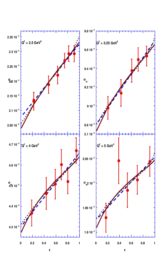
Fig. 1 shows $\sigma_{R}(\varepsilon)$ at $Q^{2}=$ 2.5, 3.25, 4.0, and 5.0 GeV², respectively, for the data from Ref. [7]. The dashed, solid, and dotted lines, correspond to the results of the fits I, II, and III, respectively. The dashed lines are straight lines and the dotted lines and the solid lines have small curvatures. One sees that both of the solid and dotted lines, in the range of $0.2<\varepsilon<0.95$, are close to the dashed lines and both of them show very little nonlinearity which agrees with the previous analyses [15, 16]. It is interesting to see that even though the $1\gamma\otimes 2\gamma$ interference term $F$ is in principle not a linear function of $\varepsilon$, it contributes significantly to the slope but very little to the curvature in fits II and III. Furthermore, we observe that outside the current data region, the dotted lines show larger nonlinearity than the solid lines at very high $\varepsilon$ region ($\varepsilon>0.95)$ . Hence, if the logarithm type functions play important role then the nonlinearity of $\sigma_{R}$ will become more pronounced at $\varepsilon>0.95$. On the other hand, in the region of $\varepsilon<0.2$, the solid lines show larger nonlinearity than the dotted lines. The nonlinearity of both solid and dotted lines are too small as compared to the uncertainty of the current data.

Figure 1: The reduced cross section $\sigma_{R}$ at $Q^{2}=1.75$ $GeV^{2}$. The dashed line is the Rosenbluth fit. The solid line represents the fit II. The dotted line represents the fit III.

To estimate the contribution of the TPE effect to the slope of $\sigma_{R}(\varepsilon)$, one can expand Eqs. (9) and (11) around $\varepsilon=1/2$ as in  [16]:

$$\sigma_{R}(\varepsilon)=\left(G_{M}^{2}+\frac{G_{E}^{2}}{2\tau}+C_{0}\right)+\left(\frac{G_{E}^{2}}{\tau}+C_{1}\right)\left(\varepsilon-\frac{1}{2}\right)+C_{2}\left(\varepsilon-\frac{1}{2}\right)^{2}+{\cal O}((\varepsilon-\frac{1}{2})^{3}),$$ (13)

where $C_{0},C_{1},$ and $C_{2}$ arise from the interference term $F$. In fit II, one has

$$C_{0}=\frac{A+3B}{\sqrt{3}},\,\,C_{1}=\frac{4(A+B)}{3\sqrt{3}},\,\,\,C_{2}=\frac{16B}{9\sqrt{3}},$$ (14)

while in the fit III, one has

$$C_{0}=\frac{4\hat{A}+\ln^{2}3\hat{B}}{4\sqrt{3}},\,\,C_{1}=\frac{4\hat{A}+(4\ln 3-\ln^{2}3)\hat{B}}{3\sqrt{3}},\,\,\,C_{2}=\frac{(16-8\ln 3)\hat{B}}{9\sqrt{3}}.$$ (15)

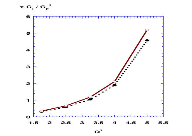
The value of $C_{0}$ is related to the contribution of the TPE effect to the intercept of $\sigma_{R}$. $C_{1}$ represents the TPE contribution to the slope of $\sigma_{R}$. $C_{2}$ reflects the curvature of $\sigma_{R}$. Fig. 2 shows the value of $C_{1}/(G_{E}^{2}/\tau)$ as a function of $Q^{2}$, which represents the ratio between the contributions of the TPE and the OPE effects to the slope of $\sigma_{R}$, for both fits II and III. One sees that the value of $C_{1}/(G_{E}^{2}/\tau)$ increases from a value of $\sim 0.3$ at $Q^{2}=1.75\,GeV^{2}$ to about $4-6$ at $Q^{2}=5\,GeV^{2}$, a huge effect. On the other hand, the value of $C_{0}/G_{M}^{2}$ remains small. We stress that it is $G_{E}$ term, not $G_{M}$ term one should look for the TPE effect because the contribution of the TPE effect to the cross section is only few percents but it dramatically changes the slope of the Rosenbluth plots at high $Q^{2}$. If one neglects the TPE effect, the values of $G_{E}$ will be greatly overestimated at large $Q^{2}$. It is interesting to observe that $A\,(\hat{A})$ never appears in $C_{2}$, the coefficient of $(\varepsilon-1/2)^{2}$. In [16], the following form has been adopted in their analysis,

$$\sigma_{R}=P_{0}\cdot\left[1+P_{1}(\varepsilon-\frac{1}{2})+P_{2}(\varepsilon-\frac{1}{2})^{2}\right],$$ (16)

and they obtained a very small $P_{2}$. It is not difficult to understand this result because $P_{2}$ corresponds to $C_{2}/C_{0}$ which is proportional to the ratio between $B\,(\hat{B})$ and $G_{M}^{2}$. In addition, one notes that if $B\,(\hat{B})=0$, then $P_{2}$ is identically equal to zero. In that case one needs to expand $\sigma_{R}$ up to ${\cal O}(\varepsilon^{3})$. The values of $P_{2}$ are around a few percent as seen in Tables 4 and 5, which agree with the findings in [15, 16]. In general the values of $P_{2}$ obtained in fit II are about three times as large as those of the fit III and they increase slowly with $Q^{2}$.

Figure 2: The values of $C_{1}/(\frac{1}{\tau}G_{E}^{2})$ in the fit II and III. The solid line represents the fit II and the dashed line represents the fit III.

Figure 3: The ratio $R^{\pm}$ of the positron-proton and electron-proton scattering cross section according to the fit II (left panel) and fit III (right panel). The dotted, dashed, and solid curves correspond to results of $Q^{2}=1.75,3.25,$ and $5.0\,GeV^{2}$, respectively.

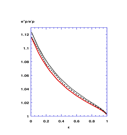
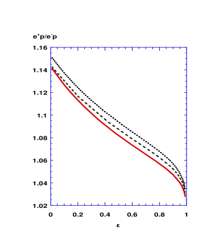
For positron-proton scattering the interference term between the one-photon and the two-photon exchange amplitudes changes sign and yields a ratio $R^{\pm}=\sigma(e^{+}p)/\sigma(e^{-}p)\approx 1+4Re(A^{2\gamma}/A^{1\gamma})$, where $A^{2\gamma}$ and $A^{1\gamma}$ are the two-photon and one-photon exchange amplitudes, respectively. Owing to the low luminosity of the secondary positron beams, almost all the comparisons were made at very low $Q^{2}$, or at small scattering angels, corresponding to $\varepsilon>0.7$. New positron measurements [18] will be performed in the near future to measure the TPE effect at larger angels and moderate $Q^{2}$ values. Here we present our $R^{\pm}$ in Fig. 3 for fits II and III, where dotted, dashed, and solid lines correspond to results of $Q^{2}=1.75,3.25,$ and $5\,GeV^{2}$, respectively. Indeed at low $Q^{2}$ and high $\varepsilon$ region, the $R^{\pm}$ is smaller than a few percent. The values of $R^{\pm}$ are not sensitive to the values of $Q^{2}$, for example, in fit II, the value corresponding to $Q^{2}=1.75\,GeV^{2}$ is about $2\%$ lower than the one at $Q^{2}=5\,GeV^{2}$. The situation is very different at lower $\varepsilon$ region. The value of $R^{\pm}$ would reach more than $10\%$ at moderate $Q^{2}\,\geq\,1.75\,GeV^{2}$, for both fits II and III, in the region $\varepsilon<0.4$. Consequently the new positron measurements [18] will very likely shed new light of the TPE effect in the $ep$ scattering if the experimental uncertainty can be reduced with $5\%$ and the $\varepsilon$ can reach 0.4 or below.

In summary, we re-analyze the data of the elastic electron proton scattering to look for model-independent evidence of the two-photon-exchange (TPE) effect. In contrast to previous analysis of [15], we parametrize the TPE effect in forms which are free of kinematical-singularity, in addition to being consistent with the constraint imposed by crossing symmetry and the charge conjugation. Moreover, we fix the value of $R=G_{E}/G_{M}$ as determined from the data of the polarization transfer experiment. We find that the TPE effect in the slope of $\sigma_{R}(\varepsilon)$, starting at high $Q^{2}\sim 2\,GeV^{2}$ values, is large and comparable with that coming from $G_{E}$ in the elastic cross section of $ep$ scattering. It becomes dominant when $Q^{2}$ reaches $\geq 4\,GeV^{2}$. In addition, the TPE effect is found to behave quasi-linearly in the region of the current data, i.e., $0.2<\varepsilon<0.95$. It explains why the previous fits do not find clear evidence for the nonlinearity in the data of $\sigma_{R}(\varepsilon)$. Hence the fact that the current elastic $ep$ cross section data shows little nonlinearity with respect to $\varepsilon$ can not be used to exclude the presence of the TPE effect.

Our values of $G_{E}$ is much smaller than the results of the Rosenbluth fit. On the other hand, our values of $G_{M}$ are about $2\%$ larger than the results of the Rosenbluth fit. The ratio of the positron-proton and the electron-proton scattering cross section is also estimated according to our parametrizations. We find that the value of $R^{\pm}$ would reach more than $10\%$ at moderate $Q^{2}\,\geq\,1.75\,GeV^{2}$ in the region $\varepsilon<0.4$ which would be of interest for future experimental planning. More precise data taken outside the region of the current data $\varepsilon<0.2$ or $\varepsilon>0.95$ will be required to distinguish the different parameterizations of the TPE effect.

Acknowledgements

This work is partially supported by the National Science Council of Taiwan under grants nos. NSC095-2112-M022-025 (S.N.Y. and Y.C.C.) and NSC095-2112-M033-014 (C.W.K.). We thank J. Arrington for providing us with the data sets and E. Tomasi-Gustafsson for helpful communications.

References

- [1] A.I. Akhiezer and M.P. Rekalo, Sov. J. Part. Nucl. 3, 277 (1974); R. Arnold, C. Carlson, and F. Gross, Phys. Rev. C 23, 363 (1981.
- [2] M. K. Jones et al. Phys. Rev. Lett. 84, 1398 (2002).
- [3] O. Gayou et al., Phys. Rev. Lett. 88, 092301 (2002); O. Gayou et al., Phys. Rev. C 64, 038202 (2001).
- [4] M. E. Christy et al., Phys. Rev. C 70, 015206 (2004).
- [5] A. Qattan et al., Phys. Rev. Lett. 94, 142301 (2005).
- [6] R.C. Walker et al., Phys. Rev. D 49, 5671 (1994).
- [7] L. Andivahis et al., Phys. Rev. D 50, 5491 (1994).
- [8] P. A. M. Guichon and M. Vanderhaeghen, Phys. Rev. Lett. 91, 142303 (2003).
- [9] P. G. Blunden, W. Melnitchouk and J. A. Tjon, Phys. Rev. Lett. 91, 142304 (2003).
- [10] Y. C. Chen, A. Afanasev, S. J. Brodsky, C. E. Carlson and M. Vanderhaeghen, Phys. Rev. Lett. 93, 122301 (2004); A. Afanasev, S. J. Brodsky, C. E. Carlson, Y. C. Chen and M. Vanderhaeghen, Phys. Rev. D 72, 013008 (2005).
- [11] L.W. Mo and Y. -S. Tsai, Rev. Mod. Phys. 41, 205 (1969).
- [12] S.P. Wells et al. (SAMPLE), Phys. Rev. C 63, 064001 (2001).
- [13] F.E. Maas et al. Phys. Rev. Lett. 94 082001 (2005).
- [14] P. G. Blunden, W. Melnitchouk and J. A. Tjon, Phys. Rev. C 72, 034612 (2005).
- [15] E. Tomasi-Gustafsson and G. I. Gak, Phys. Rev. C 72, 015209 (2005).
- [16] V. Tvaskis et al., Phys. Rev. C 73, 025206 (2006).
- [17] M. P. Rekalo and E. Tomasi-Gustafsson, Eur. Phys. J. A. 22, 331 (2004).
- [18] J. Arrington et al., nucl-ex/0408020; Jefferson Lab. experiments E-04-116, contact person, W. Brooks.