Equation of State of Nuclear Matter at high baryon density
Abstract
A central issue in the theory of astrophysical compact objects and heavy ion reactions at intermediate and relativistic energies is the Nuclear Equation of State (EoS). On one hand, the large and expanding set of experimental and observational data is expected to constrain the behaviour of the nuclear EoS, especially at density above saturation, where it is directly linked to fundamental processes which can occur in dense matter. On the other hand, theoretical predictions for the EoS at high density can be challenged by the phenomenological findings. In this topical review paper we present the many-body theory of nuclear matter as developed along different years and with different methods. Only nucleonic degrees of freedom are considered. We compare the different methods at formal level, as well as the final EoS calculated within each one of the considered many-body schemes. The outcome of this analysis should help in restricting the uncertainty of the theoretical predictions for the nuclear EoS.
1 Introduction
The knowledge of the nuclear Equation of State (EoS) is one of the fundamental goals in nuclear physics which has not yet been achieved. The possibility to extract information on the nuclear EoS, in particular at high baryon density, is restricted to two fields of research. The interplay between the theory and the observations of astrophysical compact objects is of great relevance in constraining the nuclear EoS. The enormous work that has been developing since the last two decades on the study of heavy ion reactions at intermediate and relativistic energies is the other pillar on which one can hope two build a reasonable model of the nuclear EoS. On the other hand, theoretical predictions of the EoS are essential for modeling heavy ion collisions, at intermediate and relativistic energies, and the structure of neutron stars, supernova explosions, binary collisions of compact stellar objects and their interactions with black holes. In the astrophysical context the dynamics is slow enough and the size scale large enough to ensure the local equilibrium of nuclear matter, i.e. hydrodynamics can be applied, and therefore the very concept of EoS is extremely useful. On the contrary, in nuclear collisions the time scale is the typical one for nuclear processes and the size of the system is only one order of magnitude larger than the interaction range or possibly of the particle mean free path. The physical conditions in the two contexts are therefore quite different. Despite that, by a careful analysis of experimental data on heavy ion collisions and astrophysical observations it is possible to connect the two realms of phenomena which involve nuclear processes at fundamental level, and the EoS provides the crucial concept to establish this link.
From the theoretical point of view the microscopic theory of nuclear matter has a long history and impressive progress has been made along the years. In this topical review paper we will first review the many-body theory of nuclear matter and compare the predictions of different approaches, Sec. 2-8. In Sections 9-10 possible hints from astrophysical observations and heavy ion reactions on the nuclear EoS will be critically reviewed, with emphasis on the connections that can be established between the two fields.
2 Many-body theory of the EoS.
The many-body theory of nuclear matter, where only nucleonic degrees of freedom are considered, has developed since several decades along different lines and methods. We summarize the most recent results in this field and compare the different methods at formal level, as well as the final EoS calculated within each one of the considered many-body schemes. The outcome of this analysis should help in restricting the uncertainty of the theoretical predictions for the nuclear EoS.
Within the non–relativistic approach the main microscopic methods are the Bethe–Brueckner–Goldstone (BBG) approach and the variational method (VM). The Bethe–Brueckner–Goldstone is a general many-body method particularly suited for nuclear systems. It has been extensively applied to homogeneous nuclear matter since many years and it has been presented in several review articles and textbooks. For a pedagogical review see Baldo (1999), where a short historical introduction and extended references can be found. Here we restrict the presentation to the basic structure of the method, but we will go to some detail in order to prepare the material needed for a formal comparison with other methods. We follow closely the presentation of Baldo (1999), at least for the more elementary parts.
Let us suppose for the moment that only a two-body interaction is present. Then the Hamiltonian can be written
| (1) |
where the operators () are the usual creation (annihilation) operators. The state label includes both the three-momentum and the spin-isospin variables of the single particle state. As usual we will represent the interaction matrix elements as in Fig. 1, where a particle (hole) state is represented by a line with an up (down) arrow.
To be definite, for a purely central local interaction the matrix elements read, in general
| (2) |
where the ’s are the single particle wave functions. The graph of Fig. 1 can be interpreted as an interaction of the particle and the hole which scatter after the interaction to and respectively. Incoming arrows in Fig. 1 correspond to states appearing on the right of the matrix elements, while the first (second) dot indicates their position in the two-body state.
These graphs for the matrix elements of are the building blocks for the more complete graphs representing the energy perturbation expansion.
The starting point of the perturbation expansion is the Gell-Mann and Low theorem (Gell-Mann and Low 1951). The theorem is quite general and applies to all systems which possess a non-degenerate ground state (with a finite energy). If we call the ground state of the full Hamiltonian , the theorem states that it can be obtained from the ground state of the unperturbed Hamiltonian (in our case the free Fermi gas ground state) by a procedure usually called the adiabatic “switching on” of the interaction
| (3) |
which entails the normalization . In Eq. (3), is the evolution operator, in the interaction picture, from the generic time to the time of the modified Hamiltonian
| (4) |
where . Equation (4) implies that the Hamiltonian coincides with in the limit and with at and that the interaction is switched on following an infinitely slow evolution, namely, adiabatically. Equation (3) includes also the limit . The order of the two limits is of course essential and cannot be interchanged.
Intuitively the content of the Gell-Mann and Low theorem is simple: if the Hamiltonian evolves adiabatically and if we start from the ground state of the Hamiltonian at a given initial time , the system will remain in the ground state of the local Hamiltonian at any subsequent time , since an infinitely slow evolution cannot excite any system by a finite amount of energy. It is therefore essential for the validity of the theorem that, during the evolution, the local ground state never becomes degenerate, e.g. no phase transition occurs. In the latter case, Eq. (3) will provide a state which is not the ground state of but the state which can be obtained smoothly from the unperturbed ground state through the adiabatic switching on of the interaction.
The operator can be obtained by a perturbation expansion from the free evolution operator , and for the present purpose one can write
| (5) |
where is the time ordered operator and
| (6) |
In Eq. (6) the indication of the dependence of on was omitted for simplicity. The limit has to be taken after all the necessary manipulations have been performed. The demonstration of the Gell-Mann and Low theorem, based on the expansion of Eq. (5), can be found in the original paper or in textbooks on general many-body theory (Fetter and Walecka 1971). From Eq. (3), it follows that the energy shift due to the nucleon–nucleon interaction is given by
| (7) |
where the expansion of Eq. (5) has to be used both in the numerator and in the denominator. The procedure is ill-defined in the limit , as one can see by considering the first non-trivial term () of the expansion of Eq. (5) and taking the matrix elements appearing in Eq. (7). They blow up in that limit. Fortunately, here we can get help from the so called “linked cluster” theorem. The formulation of the theorem is better stated in the language of the diagrammatic method, as explained below. The theorem shows that the numerator and the denominator possess a common factor, which includes all the diverging terms, and therefore they cancel out exactly, leaving a well defined finite result.
Finally, each term of the perturbation expansion can be explicitly worked out by means of Wick’ s theorem, which allows one to evaluate the mean value of an arbitrary product of annihilation and creation operators in the unperturbed ground state. Then the perturbative expansion of the interaction energy part of the ground state energy can be expressed in terms of “Goldstone diagrams”, as devised by Goldstone (1957). Each diagram represents, in a convenient graphical form, a term of the expansion, in order to avoid lengthy analytical expressions and to make their structure immediately apparent. The general rules (from i to vi below) for associating the analytical expression to a given diagram are described in the following. The expression is constructed by the following factors.
(i) Each drawing of the form of Fig. 1, which can be called conventionally a “vertex”, as usual represents a matrix element of the two-body interaction, according to the rules discussed previously.
(ii) A line with an upward (downward) arrow indicates a particle (hole) state, and it will be labeled by a momentum (including spin-isospin), a different one for each line.
(iii) Between two successive vertices a certain number of lines (holes or particles) will be present in the diagrams. Then, the energy denominator
| (8) |
is introduced, where now the summation runs only on the particle and hole energies which are present in the diagram between the two vertices.
(iv) Each diagram is given an overall sign , where is the order of the diagram in the expansion, is the total number of hole lines in the diagram, and the number of closed loops. A “loop” is a fermion line (hole or particle) which closes on itself when followed along the diagrams, as indicated by the directions of the arrows, passing eventually through the dots of vertices.
(v) Finally a “symmetry factor” of the form , , has to be put in front of the whole expression. In general, the factor is connected with the symmetry of the diagram, and to find its correct value it is necessary to analyze the formalism in more detail. Let us consider the case where two lines, both particles or both holes, connect the same two interaction vertices, without being involved in any other part of the diagram. They can be called “equivalent lines”. In this case, the only one that will be considered, the symmetry factor is .
(vi) Of course, one must finally sum over all the momenta labeling the lines of the diagram.
Since we are considering the ground state energy, only “closed” diagrams must be included, i.e. no external line must be present. Furthermore, according to the linked-cluster theorem, only connected diagrams must be considered, i.e. diagrams which cannot be separated into two or more pieces with no line joining them.
In conclusion, the ground state energy shift is obtained by summing up all possible closed and linked diagrams
| (9) |
where the subscript means connected diagrams only, linked with the first interaction . The latter specification means simply, in this case, that the diagram must be complete, namely it must involve all the interactions.
Another fundamental consequence of the restriction to connected diagrams is that the energy shift is proportional to the volume of the system, as it must be for extended systems with short range interactions only. Disconnected diagrams have the unphysical property to be proportional to higher powers of the volume.
Let us consider the nuclear matter case with a typical NN interaction. The NN interaction is characterized by a strong repulsion at short distance. The simplest assumption would be to consider an infinite hard core below a certain core radius. Such a NN potential has obviously infinite matrix elements in momentum representation, and a perturbation expansion has no meaning. All modern realistic NN interactions introduce a finite repulsive core, which however is quite large, and therefore in any case a straightforward perturbative expansion cannot be applied. The repulsive core is expected to modify strongly the ground state wave function whenever the coordinates of two particles approach each other at a separation distance smaller than the core radius . In such a situation the wave function should be sharply decreasing with the two particle distance. The “wave function” of two particles in the unperturbed ground state can be defined as ()
| (10) |
where are spin-isospin variables, and , are the center of mass and relative coordinate of the two particles respectively. Therefore the wave function of the relative motion in the -wave is proportional to the spherical Bessel function of order zero , with the modulus of the relative momentum vector . The core repulsion is expected to act mainly in the -wave, since it is short range, and therefore this behaviour must be strongly modified. In the simple case of the free wave function , and schematically one can expect a modification, due to the core, as depicted in Fig. 2.

The main effect of the core is to “deplete” the wave function close to , in a region of the order of the core radius . Of course, the attractive part of the interaction will modify this simple picture at . If the core interaction is the strongest one, then the average probability for two particles to be at distance would be a measure of the overall strength of the interaction. If is small, then one can try to expand the total energy shift in power of . The power has, in fact, the meaning of probability for particles to be all at a relative distance less than . In a very rough estimate is given by the ratio between the volume occupied by the core and the average available volume per particle
| (11) |
with . From Eq. (11) one gets , which is small at saturation, , and the commonly adopted value for the core is . The parameter remains small up to few times the saturation density.
The graphs of the expansion can now be ordered according to the order of the correlations they describe, i.e. the power in they are associated with. It is easy to recognize that this is physically equivalent to grouping the diagrams according to the number of hole lines they contain, where hole lines correspond to -body correlations. In fact, an irreducible diagram with hole lines describes a process in which particles are excited from the Fermi sea and scatter in some way above the Fermi sea. Equivalently, all the diagrams with hole lines describe the effect of clusters of particles, and therefore the arrangement of the expansion for increasing number of hole lines is called alternatively “hole expansion” or “cluster expansion”.
The series of two hole-line diagrams starts with the diagrams depicted in Fig. 3 (first order) and in Fig. 4 (second order) and continues with the ones shown in Fig. 5.
The infinite set of diagrams depicted in Fig. 5 can be summed up formally by introducing the two-body scattering matrix , as schematically indicated in Fig. 6.
In the second line of Fig. 6 the geometric series has been re-introduced, once the initial interaction has been isolated. This corresponds to the following integral equation
| (12) |
In the diagrams, the intermediate states are particle states, and this is indicated in Eq. (12) by the two factors . One can consider the diagrams of Fig. 6 as part of a given complete diagram of the total energy expansion. Therefore all the energy denominators contain the otherwise undefined quantity , usually indicated as the “entry energy” of the matrix. The precise value of will depend on the rest of the diagram where the matrix appears, as we will see soon. Equation (12) is anyhow well defined for any given value of . It has to be noticed that Eq. (12) is very similar to the equation which defines the usual off-shell scattering matrix between two particles in free space. The matrix of Eq. (12) can be considered the generalization of the matrix to the case of two particles in a medium (nuclear matter in our case). Actually in the zero density limit, and the matrix indeed coincides with the scattering matrix. Once the matrix has been introduced, the full set of two hole-line diagrams can be expressed as in Fig. 7, where the matrix is now indicated by a wiggly line.
This notation stresses the similarity between the matrix and the bare nucleon-nucleon interaction . This result, as depicted in Fig. 7, can be checked by expanding Eq. (12) (by iteration). The entry energy in this case is , which means that the matrix is “on the energy shell”, i.e. the matrix is calculated at the energy of the initial state. The diagrams need a factor , since the two hole-lines are equivalent, according to rule (v). Therefore the correction to the unperturbed total energy (just the kinetic energy), at the two hole-line level of approximation, is given by
| (13) |
where the label indicates that both direct and “exchange” matrix elements have to be considered, i.e. . One of the major virtues of the matrix is to be defined even when the interaction is singular (e.g. it presents an infinite hard core). This shows that the matrix is in some sense “smaller” than the NN interaction , and an expansion of the total energy shift in , instead of , should have a better degree of convergence. To substitute with the matrix in the original expansion is always possible, since a “ladder sum” (a set of diagrams of the type in Fig. 6) can always be inserted at a given vertex and the corresponding series of diagrams summed up (with the proviso of avoiding double counting). In general, however, the resulting -matrix will be “off the energy shell”, which complicates the calculations considerably. It turns out, anyhow, that also the bare expansion of in terms of the -matrix, in place of the NN interaction , is still badly divergent.
The solution of this problem is provided by the introduction of an “auxiliary” single particle potential . The physical reason of such a procedure becomes apparent if one notices that the energies of the hole or particle states are surely modified by the presence of the interaction , and intuitively they should have some relevant effects on the total energy of the system. However, in the Goldstone expansion of Eq. (9), or similar, such an effect does not appear explicitly, and therefore it should be somehow introduced into (or extracted from) the expansion, since, physically speaking, any two-body or higher correlations should be evaluated as corrections to some mean field contribution. The genuine strength of the correlations has to be estimated in comparison with a reference mean field energy, rather than to the free particle energy. The explicit form of the auxiliary single particle potential has to be chosen in such a way to minimize the effect of correlations, which is equivalent to speed up the rate of convergence of the expansion. Formally, one can re-write the original Hamiltonian by adding and subtracting the auxiliary single particle potential
| (14) |
and consider as the new single particle spectrum. The expansion is now in the new perturbation interaction . The final result should be, of course, not dependent on , at least in principle. A “good” choice of the auxiliary potential is surely one which is able to strongly reduce the contribution of to the total energy of the system. The perturbation expansion in can be formulated in terms of the same Goldstone diagrams discussed previously, where the single particle kinetic energies are substituted by the energies in all energy denominators. Furthermore, new terms must be introduced, which correspond to the so called “ insertions”. More precisely, the rules i-vi above must be supplemented by the following two other additional rules. (i - bis) A symbol of the form reported in Fig. 8
indicates a insertion, which corresponds to a factor in the diagram. (iv - bis) A diagram with a number of insertions contains the additional phase . This is a trivial consequence of the minus sign with which appears in .
The first insertion of Fig. 9 cancels out exactly the potential energy part of the single particle energies as contained in , see Eq. (14), and therefore the total energy at the two hole-line level is given by
| (15) |
One has to keep in mind that the matrix depends now on , since the auxiliary potential appears in the definition of the single particle energies . The appearance of the unperturbed kinetic energy is valid for any choice of the auxiliary potential and it is not modified by the addition of the higher order terms in the expansion. It is a distinctive feature of the Goldstone expansion that all correlations modify only the interaction part and leave the kinetic energy unchanged. Of course this property is pertinent only to the expression of the ground state energy.
It is time now to discuss the choice of the auxiliary potential. A good choice of should minimize the contributions from higher order correlations, i.e. the contributions of the diagrams with three or more hole-lines. In other words, the insertion diagrams must counterbalance the diagrams with no insertion. An exact cancellation is of course not possible, however one can select some graphs which are expected to be large and try to cancel them out exactly. At the three hole-line level, one of the largest contributions is expected to be given by the graph of Fig. 10a.
In this diagram the symbol, already introduced, for indicating a matrix stands for the corresponding ladder summation inside the diagram. This can be done systematically along the expansion, but one has to be careful in checking the energy at which the matrix has to be calculated, i.e. if it is on shell or off shell. It has been shown by Bethe, Brandow and Petschek (1962) that it is possible to choose in such a way that the corresponding potential insertion diagram, shown in Fig. 10b, cancels out the (hole) “bubble diagram” of Fig. 10a. This is indeed possible by virtue of the so called BBP theorem established by the authors, which states that the matrix connected with the bubble in the diagram of Fig. (10a) must be calculated on the energy shell, namely . For the other two matrices appearing in the diagram this property is also valid, but this is a trivial consequence of the theorem. Therefore, if one adopts for the auxiliary potential the choice
| (16) |
it is straightforward to see that the diagram of Fig. 10b is equal to minus the diagram of Fig. 10a (remind the rule iv - bis).
The choice of Eq. (16) for was originally devised by Brueckner, on the basis of physical considerations. The choice of Eq. (16) is therefore called the Brueckner potential; it implies a self-consistent determination of , since, as already mentioned, the matrix itself depends on . The hole expansion with the Brueckner choice for is called the Bethe–Brueckner–Goldstone (BBG) expansion.
In the original Brueckner theory the potential was assumed to be zero above . This is called the “standard choice”, or “gap choice”, since it necessarily implies that the single particle energy is discontinuous at . This choice also implies that the potential insertion diagram of Fig. 11b is automatically zero. The corresponding diagram, with the matrix replacing the auxiliary potential, depicted in Fig. 11a, is therefore in no way counterbalanced. The matrix in this diagram is off shell. In fact, the BBP theorem does not hold for it. The graph of Fig. 11a is usually referred to also as the particle bubble diagram, or simply “bubble diagram”, and in the following this terminology is adopted.
Another possible choice for the auxiliary potential is the so called “continuous choice”, where is defined by Eq. (16) for all values of . In this case the potential is continuous through the Fermi surface and can be interpreted as a single particle spectrum. Furthermore the two diagrams of Fig. 11 can have some degree of compensation, as we will see in the applications. Since the final results must be independent of the choice of the auxiliary potential, the sensitivity of the results to at a given order of the expansion can be used as a criterion for the degree of convergence reached at that level of approximation. No sensitivity would correspond to a complete convergence.
The bubble diagram of Fig. (11a) can be considered the first term of the full set of three hole-line diagrams. The two hole-line diagrams have been summed up by introducing the two-body matrix, which is the generalization to the nuclear medium of the two-body scattering matrix in free space. From Eq. (12) it is apparent that the only difference between the matrix and the free space scattering matrix is the presence of the “Pauli operator” , with the (zero temperature) Fermi distribution, and the presence of the energies in place of the kinetic energies. This has far-reaching consequences.
It is therefore conceivable that the three hole-line diagrams could be summed up by introducing some similar generalization of the scattering matrix for three particles in free space, which would correspond physically to consider the contribution of the three-body clusters. The three-body scattering problem has a long history by itself, and has been given a formal solution by Fadeev (1965). For three distinguishable particles the three-body scattering matrix is expressed as the sum of three other scattering matrices, . The scattering matrices satisfy a system of three coupled integral equations. The kernel of this set of integral equations contains explicitly the two-body scattering matrices pertaining to each possible pair of particles. Also in this case, therefore, the original two-particle interaction disappears from the equations in favor of the two-body scattering matrix. The formal reason for this substitution is the need of avoiding “disconnected processes”, which introduce spurious singularities in the equations (Fadeev 1965). For identical particles the three integral equations reduce to one, because of symmetry. In fact, the three functions must coincide within a change of variable with a unique function, which we can still call . The analogous equation and scattering matrix in the case of nuclear matter (or other many-body systems in general) has been introduced by Rajaraman and Bethe (1967). The integral equation, the Bethe–Fadeev equation, reads schematically
| (17) |
The factor is the analogous of the similar factor appearing in the integral equation for the two-body scattering matrix , see Eq. (12). Therefore, the projection operator imposes that all the three particle states lie above the Fermi energy, and the denominator is the appropriate energy denominator, namely the energy of the three-particle intermediate state minus the entry energy , in close analogy with the equation for the two-body scattering matrix , Eq. (12). The real novelty with respect to the two-body case is the operator . This operator interchanges particle with particle and with particle , , where indicates the operation of cyclic permutation of its indices. It gives rise to the so-called “endemic factor” in the Fadeev equations, since it is an unavoidable complication intrinsic to the three-body problem in general. The reason for the appearance of the operator in this context is that no two successive matrices can be present in the same pair of particle lines, since the matrix already sums up all the two-body ladder processes. In other words, the matrices must alternate from one pair of particle lines to another, in all possible ways, as it is indeed apparent from the expansion by iteration of Eq. (17), which is represented in Fig. 12.
Therefore, both cyclic operations are necessary in order to include all possible processes. In the structure of Eq. (17) the third particle, with initial momentum , is somehow singled out from the other two. This choice is arbitrary, but it is done in view of the use of the Bethe–Fadeev equation within the BBG expansion.
In order to see how the introduction of the three-body scattering matrix allows one to sum up the three hole line diagrams, we first notice, following Day (1981), that this set of diagrams can be divided into two distinct groups. The first one includes the graphs where two hole lines, out of three, originate at the first interaction of the graph and terminate at the last one without any further interaction in between. Schematically the sum of this group of diagrams can be represented as in Fig. 13a.
The third hole line has been explicitly indicated, out from the rest of the diagram. The remaining part of the diagram describes the scattering, in all possible ways, of three particle lines, since no further hole line must be present in the diagram. This part of the diagram is indeed the three-body scattering matrix , and the operator in Eq. (17) ensures, as already mentioned, that only particle lines are included.
The second group includes the diagrams where two of the hole lines enter their second interaction at two different vertices in the diagram, as represented in Fig. 13b. Again the remaining part of the diagram is , i.e. the sum of the amplitudes for all possible scattering process of three particles. It is easily seen that no other structure is possible. The set of diagrams indicated in Fig. 13b can be obtained by the ones of Fig. 13a by simply interchanging the final (or initial) point of one of the “undisturbed” hole lines with the final (or initial) point of the third hole line. This means that one can obtain each graph of the group depicted in Fig. 13b by acting with the operator on the bottom of the corresponding graph of Fig. 13a. In this sense the diagrams of Fig. 13b can be considered the “exchange” diagrams of the ones in Fig. 13a (not to be confused with the term “exchange” previously introduced for the matrix elements of ). If one inserts the terms obtained by iterating Eq. (17) inside these diagrams in substitution of the scattering matrix (the box in Fig. 13), the first diagram, coming from the inhomogeneous term in Eq. (17) is just the bubble diagram of Fig. 11a. The corresponding exchange diagram is the so called “ring diagram”, reported in Fig. 14.
It turns out that for numerical reasons it is convenient to separate both bubble and ring diagrams from the rest of the three hole–line diagrams, which will be conventionally indicated as “higher” diagrams.
Indeed, going on with the iterations, one gets sets of diagrams as the ones depicted in Figs. 15, and so on.
To these series of diagrams one has, of course, to add the diagrams obtained by introducing the exchange matrix elements of in place of the direct ones (if they really introduce a new diagram). The structure of the diagrams of Figs. (15) displays indeed the successive three-particle scattering processes.
Let us notice that the graph of Fig. 10a, where the bubble is attached to the hole line, is not included, and it has to be added separately, as previously discussed in connection with the insertion diagrams.
Some ambiguity arise if the diagram of Fig. 16 should be included at the three hole-line level or not. The diagram is usually referred to as the “hole-hole” diagram, for obvious reasons. Although, due to momentum conservation, only three hole lines are independent, we will consider this particular diagram as belonging to the four hole-line class.
For writing down explicitly the three hole-line contribution to the total energy we still need to find out the correct symmetry factors and signs. Let us first consider the part of the diagram which describes the interaction among the three particle lines. In the scattering processes each two-body matrix can involve both the direct and the exchange term, as illustrated in Fig. 17. Hence, there is no additional symmetry factor involved. The three lines, in fact, are never equivalent, since the various matrices are alternating among the different possible pairs of particles along the diagram. Therefore, the direct and exchange matrix elements of each matrix have to be considered and no symmetry factor for this part of the diagram has to be introduced.
Let us consider now the hole lines which close the diagram. For the diagrams of the type of Fig. 13a, two equivalent hole lines appear, joining the first and the last interaction. As discussed previously, this implies the introduction of a symmetry factor equal to in front of each diagram belonging to this group. In conclusion, the explicit expression for the contribution of the whole set of diagrams of Fig. (13a) (the “direct” diagrams) can be written
| (18) |
where again the operators are introduced in order to generate all possible scattering processes, with the condition that the matrices alternate, from one interaction to the next one, among the possible pairs out of the three particle lines. In Eq. (18) the denominator , and analogously .
Let us now consider the exchange diagrams of Fig. 13b. They can be obtained by interchanging the initial point (or end point) of the hole line labeled with the one of the hole line , i.e. by multiplying by the expression of Eq. (18) (at the right or left side). In this case, however, we have to omit the symmetry factor , since no pair of equivalent lines appears any more. We could equally well interchange with , since in this way we actually consider the same set of diagrams. This can be readily checked by displaying explicitly the sets of associated diagrams in the two cases. It is then convenient to take the average of the two possibilities, which is equivalent to multiply by the expression of Eq. (18) and to reintroduce the factor . In summary, the entire set of three hole-line diagrams can be obtained by multiplying the expression of Eq. (18) by .
It is convenient in Eqs. (17) and (18) to single out the first interaction which occurs in , where the third hole line must originate. Posing , or, explicitly
| (19) |
then the matrix satisfies the formal equation
| (20) |
Notice that, contrary to the -matrices appearing in Eq. (13), the matrix appearing in Eq. (20) is off-the energy shell, since the denominators which enter in its definition contain the energy of the hole lines , as well as of the third particle line. The denominator is the energy of the appropriate three particles–three holes intermediate state.
Summarizing, the three–hole line contribution can be obtained by solving the integral equation (20) and inserting the solution in Eq. (18). Notice that the solution depends parametrically on the external three hole lines momenta.
The scattering matrix (or equivalently ) can be used as the building block for the construction of the irreducible four-body scattering matrix , in an analogous way as the two-body scattering matrix has been used to construct . The resulting equations for , in the case of four particles in free space, are called Yakubovsky equations. It is not difficult to imagine that additional complexities are involved in these equations. Since nobody till now has dared to write down these equations for nuclear matter, not to say to solve them, we will not discuss their structure. However, estimates of the four-hole lines contribution have been considered (Day 1981).
3 Nuclear matter within the BBG expansion.
Before summarizing the theoretical results for the EoS at zero temperature on the basis of the BBG expansion, let us briefly analyze in more detail the properties of the scattering matrix . As already mentioned, the matrix can be considered as the in medium two-body scattering matrix. This can be more clearly seen by introducing the-two body scattering wave function in analogy to the case of free space scattering (Newton 1966)
| (21) |
where we have used the relationship . The latter is obtained by multiplying by the first of Eqs. (21), which defines the scattering wave function , and making use of the integral equation (12) for the matrix. It is instructive to look more closely to the scattering wave function in coordinate representation. The centre of mass motion separates, since the total momentum is a constant of the motion. In the notation of Eq. (10), the integral equation for the scattering wave function, in the relative coordinate, reads
| (22) |
where, for simplicity, the spin–isospin indices have been suppressed and the NN interaction has been assumed to be local. Still the wave function depends on both the total momentum and on the entry energy . The latter appears in the denominator , see Eq. (12), while the total momentum appears also in the Pauli operator . The kernel in Eq. (22) is the same as in the usual theory of two-body scattering (Newton 1966), except for the Pauli operator , which has a deep consequence on the properties of . This can be most easily seen if one considers the case and an entry energy corresponding to two particles inside the Fermi sphere, . In this case the Pauli operator simply implies that the relative momentum , and the kernel reads, after a little algebra
| (23) |
where the energy denominator never vanishes (provided the energy is an increasing function of , as it always happens in practice). In the usual scattering theory (Newton 1966), on the contrary, the denominator can vanish and the integral on provides the free one particle Green’ s function (according to the chosen boundary conditions). Then, for large values of , one gets the usual asymptotic behaviour (for outgoing boundary condition)
| (24) |
which describes an outgoing spherical wave and therefore a flux of scattered particles. Here is the angle between and the initial momentum . The asymptotic behaviour of the kernel of Eq. (22) can be obtained by a first partial integration with respect to the sine function
| (25) |
since further partial integrations give higher inverse power of (here the non-vanishing of the energy denominator is essential). The asymptotic behaviour of follows easily from Eq. (25), since the NN interaction is of short range. Inserting Eq. (25) in Eq. (22), one gets
| (26) |
In this case the scattered flux vanishes at large distance, since the scattered wave vanishes faster than , and no real scattering actually occurs. The scattering wave function indeed merges, at large distance , into the two-body relative wave function of Eq. (10) for a gas of free particles. In the language of scattering theory this means that all the phase shifts are zero. This property is usually called the “re-phasing” of the function . The two-body wave function does not describe a scattering process but rather the distortion of the two-body relative motion due to the interaction with respect to free gas case. Since the interaction is assumed to be of short range, such a distortion is concentrated at short distance, mainly inside the repulsive core region, but also slightly outside it (due to the attractive part of the interaction and to quantal effects).
It has to be stressed that for entry energy corresponding to two particles above the Fermi sphere, the two-body wave function can be still defined, as well as the scattering matrix, and this is indeed necessary for the continuous choice of the auxiliary potential . In this case can describe a real scattering (the energy denominator can vanish), namely a collision process of two particles inside nuclear matter, provided the correct boundary condition is imposed. This is always the case when the two particles initial momenta lie above the Fermi sphere.

Let us go back to the case of two particles inside the Fermi sphere. The difference between the wave function and the corresponding free wave function , already introduced, Eq. (10), is called the “defect function” . The size of the defect function is a measure of the two-body correlations present in the system. As a more quantitative parameter one can take the norm of the defect function, averaged over the Fermi sphere and calculated inside the available volume per particle. The parameter is usually called “wound parameter”, since it describes the “wound” in the wave function produced by the NN correlations, and it is a more refined version of the parameter previously introduced in discussing the hole expansion. Since the repulsive core is expected to have the dominant effect in nuclear matter, and it is of short range, the -wave component of should be the most affected one, and therefore the corresponding defect function should be the largest one. This is indeed the case, as shown in Fig. 18, where the function in the channel (Eqs. (21) and (22) can be easily written in spin-isospin coupled representation), is reported (dots) in comparison with the corresponding free relative wave function (full line). The calculations have been done in the continuous choice and at saturation density . The initial relative momentum was chosen at (the value at exactly can create numerical problems). One can see that the distortion of the free wave function is concentrated at small values (the square of the wave function has to be taken). One can notice the striking similarity with the naive guess of Fig. 2. At distance larger than the core radius the correlated wave function oscillates slightly around the uncorrelated one, an effect mostly due to the large distance attractive component of the NN interaction.
The short distance correlation is expected to decrease for higher partial waves. It should also be affected by the initial relative momentum. Both effects are shown in Fig. 19, where the two-body wave function at relative momentum is reported for the and channels.

The “healing effect” is apparent in all these cases, the two-body relative wave function is strongly suppressed at short distance. The corresponding “healing distance”, the size of the interval where the suppression occurs, can be used to estimate the wound parameter, as discussed above. Values of this parameter are about 0.2-0.25 around saturation density for symmetric nuclear matter, which indicate a moderate rate of convergence. Even at densities of few times the saturation value the wound parameter does not exceed 0.3 - 0.35. In pure neutron matter it turns out that the wound parameter is smaller by about a factor 2 in the same density range, and convergence should be much better.
It has to be stressed, anyhow, that the reduction of weight that should be obtained by an additional hole line in the set of diagrams along the BBG expansion does not depend only on the probability to find two particles at short distance, but also on the action of the NN potential on the defect function . Since the introduction of the scattering -matrix should take care, to a large extent, of the short range correlations due to the repulsive core, the higher order correlations should contain a more balanced contribution from the repulsive and attractive parts of the interaction, and therefore a strong compensation between attractive and repulsive contributions to the expansion. With some degree of optimism, one can hope that the expansion rate could be even better than the one guessed from the value of the wound parameter.
This expectation is indeed confirmed by actual calculations of the three hole-line contributions. The results of Baldo et al. (2001) are reported in Fig. 20 for the Argonne v18 NN potential (Wiringa et al. 1995), and symmetric nuclear matter, both for the gap and for the continuous choice. The full lines correspond to the Brueckner two hole-line level of approximation (Brueckner-Hartree-Fock or BHF), while the symbols indicate results obtained adding the three hole-line contributions.

Two conclusions can be drawn from these results.
i) At the Brueckner level the gap and continuous choice still differ by few MeV, which indicates that the results depend to a certain extent on the choice of the auxiliary potential. According to the discussion above this implies that the expansion has not yet reached full convergence. On the contrary when the three hole-line diagrams are added the results with the different choices for the single particle potential are quite close, which is surely an indication that the expansion has reached a good degree of convergence. Notice that the insensitivity to the choice of is valid in a wide range of density, only at the highest density some discrepancy starts to appear. One can see that even at 4-5 times saturation density the BBG expansion can be considered reliable. ii) As already discussed, the auxiliary potential is crucial for the convergence of the BBG expansion. It is not surprising, therefore, that the rate of convergence is dependent on the particular choice of . From the results it appears that the continuous choice is an optimal one, since the three hole-line corrections are much smaller and negligible in first approximation. It is important to stress that the smallness of the three hole-line corrections is the result of a strong cancellation of the contributions of the different diagrams discussed above. This is illustrated in Fig. 21, where the values of the bubble (figure 11a), ring (figure 14), U–potential insertion (11b) and higher order diagrams are reported.

This shows clearly the relevance of grouping the diagrams according to the number of hole lines, in agreement with the BBG expansion. An ordering of the diagrams according to e.g. the number of -matrices involved would be badly divergent.
Similar results are obtained for pure neutron matter, as illustrated in Fig. 22, taken from Baldo et al. (2000). Notice that, in agreement with the previous discussion on the wound parameter, the rate of convergence looks faster in this case.

4 The Coupled Cluster Method
The BBG expansion can be obtained also within the Coupled-Cluster Method (CCM) (Kümmel et al. 1978), a general many-body theory which has been extensively applied in a wide variety of different physical systems, both bosonic and fermionic ones. The connection between the CCM and the BBG expansions has been clarified by Day (1983). In the CCM method one starts from a particular ansatz on the form of the exact ground state wave function in terms of the unperturbed ground state
| (27) |
where the hermitean operator is expanded in terms of n-particle and n-hole unperturbed states
| (28) |
where all the ’ s are hole momenta, i.e. inside the Fermi sphere, and all the ’ s are particle momenta, i.e. outside the Fermi sphere. For translationally invariant systems the term vanishes due to momentum conservation. The exponential form is chosen in order to include, as much as possible, only “linked” terms in the expansion of , in the spirit of the linked-cluster theorem discussed above. As already noticed, the unlinked diagrams can indeed be summed up by an exponential form. This form also implies the normalization . The functions are expected to describe the n-body correlations in the ground state. As an illustration, let us consider only for simplicity and let us assume that it can be considered local in coordinate space, , where the labels include spin-isospin variables. Then the correlated ground state can be written
| (29) |
where the product runs over all possible distinct pairs of particles and . In general, however, the functions are highly non-local in coordinate space and the expression for the ground state wave function cannot be written in such a simple form.
The eigenvalue equation for the exact ground state can be re-written as a (non-hermitean) eigenvalue equation for the unperturbed ground state with a modified Hamiltonian, transformed according to a similarity transformation generated by
| (30) |
The equations for the total energy and for the correlation functions can be obtained by multiplying systematically Eq. (30) by the unperturbed ground state, two particle-two hole states, three particle-three hole states, and so on. The multiplication by gives a particularly simple expression for the total energy. If only a two-body interaction is present, one gets
| (31) |
where is the unperturbed total (kinetic) energy, while all the other terms in the expansion of the similarity transformation actually vanish. Therefore, in principle the exact total energy can be obtained from the knowledge of the exact two particle- two hole amplitude only. More explicitly
| (32) |
where
| (33) |
Of course, the amplitude is connected with the higher order amplitudes . As mentioned above, the equations linking the lowest order amplitudes with the higher ones are obtained by multiplying Eq. (30) by the unperturbed particle- holes bra states (n larger or equal to 2). These equations are the constitutive “Coupled Cluster” equations, which are equivalent to the eigenvalue equation for the ground state. Approximations can be obtained by truncating this chain of equations to a certain order , i.e. neglecting for . The meaning of the truncation can be read from the ansatz Eq. (27), it amounts to consider correlated particle hole components in the ground state up to , while higher order components with are just antisymmetrized products of the lower ones (note the exponential form, which produces components of arbitrary higher orders).
This form of the CCM equations can be also obtained from the variational principle, i.e. by demanding that the mean value of the Hamiltonian in the ground state of Eq. (27) is stationary under an arbitrary variation of the state vector orthogonal to . Such a variation can be written
| (34) |
where corresponds to an arbitrary variation of the function in Eq. (28). It is easily verified that such a variation is indeed orthogonal to . This is equivalent to take systematically proportional to a particle - hole operator, for all non-zero , and to require that the corresponding energy variation vanishes. This set of conditions gives for the functions the same CCM equations, which are therefore variational in character. The energy can be still taken from Eq. (31), but variants are possible (Navarro 2002).
However, the CCM equations, as they stand, cannot be applied to calculations in nuclear matter or in nuclei. The main correlations in nuclear systems come from the strong short range repulsive core, and this part of the NN interaction requires special treatment. The many-body wave functions must take into account the overall strong repulsion which is present whenever two particles approach each other at a distance smaller than the core radius. This requirement must be incorporated systematically in the correlation functions , otherwise no truncation of the expansion would be feasible. The simplest way to proceed is to renormalize the original NN interaction and introduce an effective interaction which takes into account the two-body short range correlations from the start, so that all the remaining contributions of the expansion are expressed in terms of the renormalized, and hopefully “reduced”, interaction. In the BBG expansion this is done by introducing the G-matrix, and a similar procedure can be followed within the CCM scheme. Originally such a line was developed by Kümmel and Lührmann (1972), and resulted in the so-called Hard Core truncation scheme. A similar procedure has been followed recently in finite nuclei (Kowalski 2004 and Dean 2004), where the G-matrix, first calculated in an extended space, is then used in the CCM scheme to calculate systematically the correlations not included in the G-matrix. The introduction of the G-matrix of course changes the order of the diagrammatic expansion in the CCM method, in particular while the original CCM scheme treats particle-particle (short range) and particle-hole correlations (long range) on the same footing, the modified CCM scheme shifts the long range part of the correlations to higher orders and introduces the G-matrix as the effective two-body interaction in the corresponding terms of the expansion. The formal scheme along this lines has been developed for nuclear matter by Day (1983).
Once this procedure is introduced, in the resulting CCM equations the variational property is of course lost, as in the case of the BBG expansion.
Furthermore, a single particle potential can also be introduced in the CCM method. While the original CCM set of equations are formally independent of at each level of truncation, the modified equations do not depend on the single particle potential only if no truncation is performed. A detailed analysis of the connection between CCM and BBG expansions was presented by Day (1983). In the modified CCM equations, one introduces the effective interaction
| (35) |
where the operator in parenthesis, if applied to the unperturbed ground state, can produce two hole states, 3 holes and 1 particle, 4 holes and two particles and so on. The subscript indicates that, in this expansion, only the terms which do not annihilate the unperturbed ground state are retained, i.e. no with or with are retained. The operator can be also expanded in particles – holes operators
| (36) |
in exactly the same fashion as the operator . The functions are related with the functions . Schematically this relation can be written
| (37) |
The modified CCM equations are obtained by the same procedure as before. The equations involves now both the functions and the functions . Together with the relationship Eq. (37), a closed set of equations is then obtained, which is again equivalent to the original eigenvalue problem for the ground state. The ground state energy is still given by Eq. (32), since the relation between and , according to Eq. (37) for , is indeed given by Eq. (33). The truncation scheme (the “Bochum” truncation scheme) is now performed on both and , i.e. the truncation at order corresponds to neglecting the functions and for . If we truncate the expansion at , only and are retained. The quantity can be readily identified with the on-shell -matrix of the BBG expansion and the function with the corresponding defect function. If the self-consistent single particle potential is introduced, one then gets at this level exactly the Brueckner approximation.
As already discussed, the -matrix can be introduced in all the terms of the Coupled-Cluster expansion. In this case each term of the expansion coincides with one diagram in the BBG method. However, it turns out that the ordering of terms according to the modified CCM truncation scheme at increasing does not coincide completely with the ordering of diagrams in the hole-line expansion, i.e. for the CCM expansion at a given truncation includes also diagrams with a number of hole lines larger than . In particular, the truncation at includes also “ring diagrams” with an arbitrary number of hole lines, i.e. the whole series of the particle-hole ring diagrams initiated by the diagram of Fig. 14, adding more and more particle–hole bubbles. These have been shown to be small (Day 1981), and therefore the CCM can be considered equivalent to the BBG expansion up to the three hole-line level of approximation.
The Coupled Cluster method gives a new insight into the structure and meaning of the hole-line expansion according to the BBG method. In fact, as we have seen the CCM is based on the ansatz (27) for the ground state wave function, and it is likely that the same structure of the ground state is underlying the BBG expansion. At Brueckner level it is then consistent to assume that the ground state wave function is given by
| (38) |
with the Brueckner defect function.
5 The variational method
The variational method for the evaluation of the ground state of many-body systems was developed since the formulation of quantum theory of atoms and molecules. It acquires a particular form in nuclear physics because of the peculiarities of the NN interaction. The strong repulsion at short distance has been treated by introducing a Jastrow-like trial wave function. The complexity of the NN interaction needs special treatment and the introduction of more complex correlation factors. Many excellent review papers exist in the literature on the variational method and its extensive use for the determination of nuclear matter EoS (Navarro et al. 2002, Pandharipande and Wiringa 1979). Here we restrict the exposition to the essential ingredients of the method to the purpose of a formal and numerical comparison with the other methods.
In the simple case of a central interaction the trial ground state wave function is written as
| (39) |
where is the unperturbed ground state wave function, properly antisymmetrized, and the product runs over all possible distinct pairs of particles. The similarity with the wave function of Eq. (29) is apparent and indicates a definite link with BBG and CCM methods. The correlation function is here determined by the variational principle, i.e. by imposing that the mean value of the Hamiltonian gets a minimum (or in general stationary point)
| (40) |
In principle this is a functional equation for the correlation function , which however can be written explicitly in a closed form only if additional suitable approximations are introduced. A practical and much used method is to assume a parametrized form for and to minimize the energy with respect to the set of parameters which constrain its form. Since, as previously discussed, the wave function is expected to decrease strongly whenever two particles are at distance smaller than the repulsive core radius of the NN interaction, the function is assumed to converge to at large distance and to go rapidly to zero as , with a shape similar to the one shown in Fig. 18 for the correlated two–body wave function. Furthermore, at distance just above the core radius a possible increase of the correlation function beyond the value is possible.
For nuclear matter it is necessary to introduce a channel dependent correlation factor, which is equivalent to assume that is actually a two-body operator . One then assumes that can be expanded in the same spin-isospin, spin-orbit and tensor operators appearing in the NN interaction. Momentum dependent operators, like spin-orbit, are usually treated separately. The product in Eq. (39) must be then symmetrized since the different terms do not commute anymore. The most flexible assumption on the ’s is to impose that they go to 1 at a given “healing” distance with zero derivative. The healing distances, which eventually can be defined for each spin-isospin and tensor channels, are then taken as variational parameters, while the functions for are determined directly from the variational procedure. In principle, the condition of energy minimum (or extremal) should produce a set of Euler-Lagrange equations which determine the correlation factors. In practice, a viable explicit form can be used only for the two-body cluster terms, as discussed below.
If the two-body NN interaction is local and central, its mean value is directly related to the pair distribution function
| (41) |
where
| (42) |
The main job in the variational method is to relate the pair distribution function to the correlation factors . In general this cannot be done exactly, and one has to rely on some suitable expansion. For the central part of the correlations, the physical quantity which describes the main perturbation with respect to the free Fermi gas is the function , which is a measure of the strength of the short range part of the correlation. One can then expand the square of the correlated wave function in the components with a given number of -factors, and correspondingly the energy mean value can be expanded in different terms, each one with a given number of -functions. If the full NN interaction is considered, also the non central component of the correlation factors, , must be included in the expansion. In this case the smallness factors are and the product , since they are expected to be small and vanish at large distance. The different terms can be represented graphically by diagrams to help their classification and identify their possible cancellations. It turns out (Fantoni and Rosati 1974) that the mean value, at least in the thermodynamic limit, is the summation of the so-called “irreducible” diagrams, in strong similarity with the linked-cluster theorem of the BBG expansion. Indeed, the reducible diagrams are canceled exactly by the expansion of the denominator in Eq. (42). The problem of calculating from the ansatz of Eq. (39) has also a strong similarity with the statistical mechanics of a classical gas at finite temperature, where different methods to sum up infinite series of diagrams in the so-called “virial expansion” have been developed, noticeably the Hypernetted Chain (HNC) summation method (Leeuwven et al. 1959).These methods can be almost literally translated to the case of boson systems. With some modifications due to the different statistics, they can be extended (Fantoni and Rosati 1974) to fermion systems (FHNC), provided in this case the correlations are taken to be only central (“Jastrow type” correlations) in Eq. (39), i.e. the correlation factors are assumed to be only dependent on the coordinates. Unfortunately, in nuclear matter, as already mentioned, correlations are of complicated structure due to the NN interaction, and the HNC method can be applied only within approximate schemes, like the Single Operator Chain (SOC) summation method (Pandharipande and Wiringa 1979, Lagaris and Pandharipande 1980, Lagaris and Pandharipande 1981), called also Variational Summation Method (VSM). In VMS only chains with a given correlation operator are considered. In general, the correlation functions are calculated at the two-body cluster level, where one gets the Euler-Lagrange coupled equations for all operator channels, that can be solved exactly for the set of correlation functions at fixed values of the “healing distances”. The index labels the different two-body operators, spin-spin, spin-isospin, tensor, and so on. The VMS method is then applied, keeping the same set of correlation functions, to calculate the total energy. The procedure is repeated for different values of the healing distances and the energy minimum is found within this parameter space. The minimization gives of course automatically the ground state wave function. The VSM allows one to include a definite class of higher order “clusters” beyond the two-body ones. However, particle clusters in the variational method are physically quite different from the ones in the CCM method as well as from the BBG ones, where particle “clusters” are defined in terms of diagrams with a given number of hole-lines, according to the hole-line expansion. This point will be discussed in the next section. Generally speaking, the summation of clusters performed by chain summations are expected to include long range correlations, while the variational procedure leading to the Euler-Lagrange equations should include mainly short range correlations. Indeed, in the low density limit the Euler-Lagrange equation reduces to the Schroedinger equation for two particles in free space.
6 A critical comparison
As it has been shown by Jackson et al. (1982), in the low density limit, where two-body correlations dominate, the Euler-Lagrange equations of the variational method are equivalent to the summation of the ladder diagrams of the BBG expansion, while the hypernetted chain summation is related to the ring diagram series. This result is actually valid only for boson systems, while for Fermi systems it holds approximately, only by means of a suitable averaging over entry energy and momenta of the diagrams appearing in the BBG expansion. Indeed, the correlation factors are at most state dependent in the variational approach, while in principle they should depend also on both energy and total momentum. In any case, due to these approximate links, it was suggested (Jackson et al. 1982) to use in many-body systems in general a “parquet” summation, where both particle-particle short range correlations and chain summations of the ring type are treated on the same footing. However, this method has never been systematically exploited in the case of nuclear matter, and therefore the approach will not be discussed here.
The most relevant difference between the BBG (or CCM) method and the variational one is the introduction of the self-consistent single particle potential, which is not explicitly introduced in the variational procedure. As already noticed, with this modification the CCM and the BBG expansion are not any more of variational character, in general, at a given level of truncation. However, at the same time a large fraction of higher order correlations are effectively embodied in the single particle potential and the speed of convergence of the expansion is substantially improved. In the variational approach the average single particle potential is implicitly built up along the cluster expansion. It is likely that this is the reason of the slow convergence in the order of the clusters included in the chain summations (Morales et al. 2002), and also for this reason the meaning of “clusters” is not straightforwardly the same in the different methods.
In the variational approach three-body correlations arise as cyclic products of three two-body factors, e.g. . This contribution has been recently (Morales et al. 2002) calculated exactly in symmetric and pure neutron matter for realistic interactions. Irreducible three-body correlations can be introduced from the start by multiplying the uncorrelated wave function not only by two-body correlation factors but also by three-body correlation factors , which will then include those three-body correlations which cannot be be expressed as product of two-body ones. As noticed by Lührmann (1975), this also indicates a difference with the BBG (and CCM) expansion, where the whole three-body correlations are included in the energy term generated by the Bethe-Fadeev equations.
Despite all these differences, some similarity of the methods appear to be present, while a more detailed comparison can be made only at the level of the numerical results.
In summary, the main differences between the variational and the BBG approaches can be identified as follows.
1. In the BBG method for the nuclear EoS the kinetic energy contribution is kept at its unperturbed value at all orders of the expansion, while all the correlations are embodied in the interaction energy part. This characteristic of the BBG method is not due to any approximation but to the expansion method, where the modification of the occupation numbers due to correlations is treated on the same footing and at the same order as the other correlation effects. In the variational method both kinetic and interaction parts are directly modified by the correlation factors.
2. The correlation factors introduced in the variational method are assumed to be essentially local, but usually state dependent. The corresponding (implicit) correlation factors in the BBG expansion are in general highly non-local and energy dependent, besides being state dependent.
3. In the BBG method the auxiliary single particle potential is introduced within the expansion in order to improve the rate of convergence. No single particle potential is introduced in the variational procedure for the calculation of the ground state energy and wave function. Of course, once the variational calculation is performed, the single particle potential can be extracted. This also should imply that the rate of convergence in terms of the order of the clusters is slower in the variational method. It was indeed shown by Morales et al. (2002) that one needs clusters at least up to order 5 to get reasonable convergence, but in principle this does not create any problem in the variational method (while in the BBG expansion it would be a disastrous difficulty). It has to be stressed anyhow that the physical meaning of “cluster” is quite different in the two methods, being more related to long range correlations in the variational scheme, to the short range ones in BBG.
Point 3 is probably the most relevant difference between the two methods, but in any case it is difficult to estimate to which extent each one of the listed differences can affect the resulting EoS.
The similarity and connection between the two methods can be found by interpreting on physical grounds the diagrammatic expansion used in each one of them. The two-body correlations are surely described by the lowest order diagram of the variational method, which corresponds to a factor , which in turn can be related to the G-matrix, i.e. to the Brueckner approximation (with the warning of point 2). The hypernetted sums, in their various form, should be connected with the series of ring diagrams starting from the one discussed in connection with the three hole-line diagrams (including an arbitrary number of loops). As mentioned above, the three-body correlations included in the Bethe-Fadeev equations can be related to the irreducible product of three factors. For boson systems all these connections are more stringent, for fermion systems like nuclear matter they are much less transparent and one has to rely on physical arguments.
7 The Equation of State from the BBG and the variational approach
The first obvious requirement any EoS must satisfy is the reproduction of the so-called “saturation point” (SP) , extracted from the fit of the mass formula to the smooth part of the binding energy of nuclei along the stability valley. To be definite, we will take the values MeV and for the energy per particle and density, respectively, as defining the SP of symmetric nuclear matter. As it is well known, no two-body force which fits the NN phase shifts was found to be able to reproduce accurately the SP. In early applications of Brueckner theory it was realized that the SP predicted by different phase-equivalent NN interactions lie inside the so-called “Coester band”, after Coester et al. (1970). The band misses the phenomenological SP, even taking into account the intrinsic uncertainty coming from the extraction procedure (different mass formulae, different fit procedures, etc.). The band indicates that either the binding energy is too small but the density is correct, or the binding energy is correct but the density is too large, see Fig. 23.

Furthermore the position along the band was related to the strength of the tensor forces, i.e. to the percentage of D-wave in the deuteron. Higher values of the strength were corresponding to the upper part of the band. However the analysis was done in the gap choice, as discussed above. The use of the continuous choice within the Brueckner method changes substantially the results, as shown in Fig. 23. If some the most modern local forces, with different deuteron D-wave percentages, are used, the SP turns out to be restricted in this case to an “island” , which however is still shifted with respect to the phenomenological SP. The discrepancy does not appear dramatic. Taking into account that the Brueckner approximation is the lowest order in the BBG scheme, this result is surely remarkable. Unfortunately, as shown in the previous section, higher order contributions, namely the three hole-line diagrams, do not change the nuclear EoS appreciably and the discrepancy still persists. The variational method gives results in full agreement with this conclusion. The deficiency is evidently not in the many-body treatment but in the adopted Hamiltonian. Two possible corrections can be devised : many-body forces (to be distinguished from many-body correlations), in particular three-body forces, and relativistic effects. As we will mention later, it is well known that the two possible corrections are actually strongly related. Here we will consider three-body forces in some detail.
First we compare in Fig. 24. the BBG and variational EoS (Akmal et al. 1998) both for symmetric matter and pure neutron matter without three-body forces in order to single out the dependence of the results on the adopted many-body scheme.

Since we focus on the high density part of the EoS, i.e. above saturation density, the comparison is displayed in a wide density range. It has to be stressed that the NN phase shifts constrain the NN two-body force up to about 350 MeV in the laboratory, which corresponds to a relative momentum of about 2 fm-1. Densities corresponding to values of larger than fall surely in the region where an extrapolation is needed and the NN force is untested. For pure neutron matter the agreement between the two theories can be considered surprisingly good up to quite high density. For symmetric matter the good agreement extends up to about 0.6 fm-3, while at higher density the variational EoS is substantially higher than the BBG one. The reason for that is unknown.
This type of agreement is still present if three-body forces (TBF) are introduced to the purpose of getting a SP in agreement with the empirical findings. This can be seen in Fig. 25 , where calculations with the Argonne v18 interaction and the Urbana model for three-body forces are presented. These TBF contain an attractive and repulsive part, whose structure is suggested by elementary processes which involve meson exchanges and three nucleons but cannot be separated into two distinct nucleon-nucleon interaction processes. These TBF are phenomenological in character since the two parameters, namely the strength of the attractive and the repulsive terms, cannot be fixed from first principles but they are adjusted to reproduce accurately experimental data. In Fig. 25 we also report (full line) the EoS of Heiselberg and Hjorth–Jensen (1999), who proposed a modification of the variational EoS of Akmal et al. (1998), which prevents its superluminal behaviour at high density (this EoS is in fact softer).

Few observations are in order. It turns out that the parameters of the three-body forces which have been fitted to data on few nucleon systems (triton, and ) have to be modified if the SP has to be reproduced within the phenomenological uncertainty. Generally speaking the repulsive part has to be reduced substantially. It could be argued that this change of parameters poses a serious problem, since if the TBF model makes sense one must keep the same parameters at all densities, otherwise higher order many-body forces should be invoked. Actually this is a false problem. In fact the discrepancy on the SP cannot be reduced more than few hundred MeV (typically 200-300 KeV), due to the intrinsic uncertainty in its position. This discrepancy remains essentially the same for few-body systems if one uses the same TBF fitted in nuclear matter, and actually the contribution of TBF in few-body systems is quite small. Therefore TBF which allow one to describe both few-body systems and the nuclear matter SP do exist, if the accuracy is kept at the level of 200-300 KeV in energy per particle, and indeed they are not unique. To try a very precise overall fit at the level of 10 KeV or better, as it is now possible in the field of few-body systems, appears definitely to be too challenging. There are surely higher order terms (four-body forces, retardation effects in the NN interaction, other relativistic effects, etc.) which could contribute at this level of precision. In fact the contribution of TBF to the energy per particle around saturation is in all cases about 1-2 MeV, while for few-body systems it is one order of magnitude smaller. Therefore a TBF tuned to fit the binding energy of few-body system with an accuracy of 1-10 KeV cannot be extended to fit nuclear matter SP, since this would correspond to a quite unbalanced fitting procedure. In other words, 100-200 KeV for the energy per particle is the limit of accuracy of the TBF model applied to the nuclear EoS in the considered wide range of density.
Secondly, it has to be noticed that once the SP is reproduced by adjusting the TBF, it turns out that the parameters are not the same in the BBG and variational methods, i.e. the TBF are not the same. Finally the way of incorporating TBF is simplified in the BBG method, namely TBF are reduced to a density dependent two-body force by a suitable average over the position and spin-isospin quantum numbers of the third particle (Grangé et al. 1989). The results presented in Fig. 25 are Brueckner calculations with TBF included following this procedure. The agreement between the two curves seems to indicate that once the SP is reproduced correctly, the full EoS is determined to a large extent up to density as high as 0.6 fm-3. However the conclusion is restricted to the particular model for the two-body and three-body forces. The possible dependence on the considered forces will be discussed in the next section.
8 Dependence on the two and three-body forces
The progress in the accuracy and extension of NN experimental data, as well as in their fit by different NN interaction models has been quite impressive. The data range up to 350 MeV in the laboratory. Going beyond this limit requires the introduction of non-nucleonic degrees of freedom (mesons, isobar resonances, etc.) and the corresponding inelastic channels. The latter possibility looks quite a complex task, and only few cases are present in the literature, notably by Ter Haar and Malfliet (1987). Since in this paper we restrict to nucleonic degrees of freedom only, we will consider NN two-body interactions which do not include explicitly mesonic or isobaric degrees of freedom. Despite that, it is a common paradigm that the NN interaction is determined, at least in an effective way, by the exchange of different mesons, and practically all modern NN interactions take inspiration for their structure by this assumption, in an explicit or implicit way. A really large set of two-body interactions has been developed along the years, but nowadays it is mandatory to restrict the possible choices to the most modern ones, since they are the only ones which fit the widest and most accurate experimental data, on one hand, and are more accurate in the fitting, on the other. One can then restrict the set of possible NN two-body interactions to the ones which fit the latest data (few thousands of data points) with an accuracy which gives a /datum close to 1. With these requirements, the number of NN interactions reduces quite a bit, and only few ones can be considered acceptable. The one which is constructed more explicitly from meson exchange processes is the recently developed CD Bonn potential by Machleidt (2001), which is the latest one of the Bonn potential series. In principle this interaction is the one with the best value. However the experimental data are not always consistent to the needed degree of accuracy and some selection must be done. In the same work one can find a detailed analysis of the different data set together with the method of selection which has been followed for the most accurate NN interactions and the values of the corresponding , if one includes the data up to the year 2000. Among the most accurate NN interactions one has to include the Argonne v18, already discussed. It is constructed by a set of two-body operators which arise naturally in meson exchange processes, but the form factors are partly phenomenological (except, of course, the one-pion exchange). This interaction has been recently modified in the and channels with the inclusion of a purely phenomenological short range non-local force, which substitutes the original potentials below 1 fm (Doleschall and Borbely 2000, Doleschall et al. 2003, Doleschall 2004), usually indicated as IS potential. This allows one to reproduce the binding energy of three and four nucleon systems very accurately without the inclusion of any TBF, at variance with the original Argonne v18. Also the radii of and are accurately reproduced, while the radius of is slightly underestimated (Lazauskas and Carbonell 2004). This potential is phase-equivalent to the original interaction, but the off-shell behaviour is modified. Finally one can mention the latest potentials of the Nijmegen group (Stocks et al. 1994). They have also the ideal value /datum 1 . However the fit was performed separately in each partial wave and the corresponding two-body operator structure cannot have the simple form as expected from meson exchange processes. This interaction will be discussed only marginally. A larger set of interactions, which includes the old NN potentials, can be found in Li K H et al. (2006), where the resulting symmetric nuclear matter EoS at BHF level are compared.
It has to be noticed that the three selected NN interactions, v18, CD Bonn and IS, give an increasingly better reproduction of the three-body binding energy and radii, and at the same time their non-locality is increasing in the same order. They are all phase equivalent to a good accuracy, so that the differences appearing in the nuclear matter EoS can be solely due to their different off-shell behaviour. It is well known (Coester et al. 1970) that phase equivalent potentials can give a quite different saturation point and overall EoS, but here the comparison is restricted to a very definite class of realistic accurate NN interactions, with an operatorial structure which is quite similar and suggested by meson exchange processes. In Fig. 26 we compare the three corresponding EoS (Baldo and Maieron 2005) at the BHF level and with the inclusion of three hole-line diagrams (no TBF). First of all one can notice that also for the CD Bonn and IS interactions the three hole-line contributions are still relatively small (especially if one compares the interaction energies at two and three hole-line levels). The convergence of the hole expansion appears to be a general feature. Furthermore, at increasing non-locality the EoS become softer and the SP tends to run away from the empirical SP and unreasonably large values for the binding energy and the SP density are obtained. In the figure two versions of the IS potential are considered, NL1, where only the channel is modified, and NL2, where also the – channel is modified. The results indicate that the problem of reproducing the empirical SP with two-body realistic and accurate interactions cannot be solved by introducing non-locality, which modifies the off-shell properties of the two-body potentials. Furthermore, the requirement of a very accurate fitting of the binding energy and radii of three (and eventually four) nucleon systems makes the reproduction of nuclear matter SP more challenging.

The necessity of introducing TBF around saturation is in any case definitely confirmed. According to the results shown in Fig. 26. it is apparent that TBF cannot be unique, but they depend on the two-body forces employed, since each one of the two-body forces gives a different discrepancy for the SP and therefore needs a different correction. This is not surprising, since both two-body force and TBF should originate within the same physical framework and therefore they are intimately related. In particular, in the nucleon-meson coupling models TBF should be generated by processes which involve the coupling constants which are already present in the two-body forces. Well known examples are depicted in Fig. 8.
Fig. 27. Some processes which can contribute to three-nucleon forces.
Fig. 27. Some processes which can contribute to three-nucleon forces.
Other couplings, like meson-meson ones, appear only at the TBF level. It has to be stressed that all these processes must be considered within an effective theory framework (i.e. a theory with cutoff). The problem of consistency between two-body interactions and TBF has been taken systematically by Grangé et al (1989) and further developed in recent works (Zuo et al. 2002). Since processes which include meson-meson couplings seem to be small and can be neglected in first approximation, TBF calculated along these lines do not contain in principle any additional parameters. It is not surprising then that the corresponding EoS has a SP which is appreciably more shifted away from the empirical one if compared with the EoS with the same two-body force (v18 ) but with the phenomenological TBF (see Li Z H et al. 2006b). In any case TBF can be a good starting point for further improvements. It is unclear if other more complex processes can play a role. The effect of these TBF in few-body systems is not known, but it is expected to be not very large, since at low density also the contribution of these TBF in nuclear matter becomes quite small. The most significant difference with the phenomenological TBF is the stiffness of the EoS at high density, which turns out to be much higher, as can be seen also in the case of pure neutron matter. The energy and pressure rise steeply above saturation, and this can create some problems, as discussed later.
9 The Dirac-Brueckner approach
As already mentioned, one of the deficiencies of the Hamiltonian considered in the previous sections is the use of the non-relativistic limit. The relativistic framework is of course the framework where the nuclear EoS should be ultimately based. The best relativistic treatment developed so far is the Dirac-Brueckner approach. Excellent review papers on the method can be found in the literature (Machleidt 1989) and in textbooks (Brockmann and Machleidt 1999). Here we restrict the presentation to the main basic elements of the theory and to the latest results, in order to make the comparison with the other methods more transparent. We will follow closely the presentation by Brockmann and Machleidt (1999) but we will make reference also to the more recent developments.
In the relativistic context the only NN potentials which have been developed are the ones of OBE (one boson exchange) type. The starting point is the Lagrangian for the nucleon-mesons coupling
| (43) | |||||
| (44) | |||||
| (45) |
with the nucleon and the meson fields, where indicates the type of meson and the Lorentz component in the case of vector mesons. For isospin 1 mesons, is to be replaced by , with () the usual Pauli matrices. The labels , , , and denote pseudoscalar, pseudovector, scalar, and vector coupling/field, respectively.
The one-boson-exchange potential (OBEP) is defined as a sum of one-particle-exchange amplitudes of certain bosons with given mass and coupling. The main difference with respect to the non-relativistic case is the introduction of the Dirac-spinor amplitudes. The six non-strange bosons with masses below 1 GeV/c2 are used. Thus,
| (46) |
with and pseudoscalar, and scalar, and and vector particles. The contributions from the isovector bosons and contain a factor . In the so called static limit, i.e. treating the nucleons as infinitely heavy (their energy equals the mass) the usual denominator of the interaction amplitude in momentum space, coming from the meson propagator, is exactly the same as in the non-relativistic case (since in both cases meson kinematics is relativistic). This limit is not taken in the relativistic version, noticeably in the series of Bonn potentials, and the full expression of the amplitude with the nucleon relativistic (on-shell) energies is included. As an example, let us consider one pion exchange. As it is well known, in the non-relativistic and static limit the corresponding local potential in momentum space reads (in standard notations)
with , where and are the initial and final relative momenta of the interacting nucleons. This has to be compared with the complete expression of the matrix element between nucleonic (positive energy) states (Machleidt 2000). In the center of mass frame it reads
where are the initial and final nucleon energies. One can see that in this case some non-locality is present, since the matrix element depends separately on and . Putting , one gets again the local version. Notice that in any case the two versions coincide on-shell (), and therefore the non-locality modifies only the off-shell behaviour of the potential. The matrix elements are further implemented by form factors at the NN-meson vertices to regularize the potential and to take into account the finite size of the nucleons and the mesons. In applications of the DBHF method usually one version of the relativistic OBE potential is used, which therefore implies that a certain degree of non-locality is present. As already anticipated in the previous section, this is also true if these potentials are used within the non-relativistic BHF method.
The fully relativistic analogue of the two-body scattering matrix is the covariant Bethe-Salpeter (BS) equation. In place of the NN non-relativistic potential the sum of all connected two-particle irreducible diagrams has to be used, together with the relativistic single particle propagators. Explicitly, the BS equation for the covariant scattering matrix in an arbitrary frame can be written
| (47) |
with
| (48) | |||||
| (49) |
where , , and are the initial, intermediate, and final relative four-momenta, respectively (with e. g. ), and is the total four-momentum; . The superscripts refer to particle (1) and (2). Of course all quantities are appropriate matrices in spin (or helicity) and isospin indices. The use of the OBE potential as the kernel is equivalent to the so-called ladder approximation, where one meson exchanges occur in disjoint time intervals with respect to each other, i.e. at any time only one meson is present. Unfortunately, even in the ladder approximation the BS equation is difficult to solve since is in general non-local in time, or equivalently energy dependent, which means that the integral equation is four-dimensional. It is even not sure in general if it admits solutions. It is then customary to reduce the four-dimensional integral equation to a three-dimensional one by approximating properly the energy dependence of the kernel. In most methods the energy exchange is fixed to zero and the resulting reduced BS equation is similar to its non-relativistic counterpart. In the Thompson reduction scheme this equation for matrix elements between positive-energy spinors (c.m. frame) reads
| (50) |
where both and have to be considered as matrices acting on the two-particle helicity (or spin) space, and is the relativistic particle energy. In the alternative Blankenbecler-Sugar (Machleidt 2000) reduction scheme some different relativistic kinematical factors appear in the kernel. This shows that the reduction is not unique. The partial wave expansion of the –matrix can then be performed starting from the helicity representation. The corresponding amplitudes include single as well as coupled channels, with the same classification in quantum numbers as in the non relativistic case and therefore their connection with phase shifts is the same (Brockmann and Machleidt 1998). In the intermediate states of momentum only the positive energy states are usually considered (by the proper Dirac projection operator). As in the case of the OBEP potential, again the main difference with respect to the non-relativistic case is the use of the Dirac spinors.
The DBHF method can be developed in analogy with the non-relativistic case. The two-body correlations are described by introducing the in-medium relativistic -matrix. The DBHF scheme can be formulated as a self-consistent problem between the single particle self-energy and the -matrix. Schematically, the equations can be written
| (51) |
where is the Pauli operator which projects the intermediate two particle momenta outside the Fermi sphere, as in the BHF G-matrix equation, and is the single particle Green’ s function. The self consistency is entailed by the Dyson equation
where is the (relativistic) single particle Green’s function for a free gas of nucleons. The self-energy is a matrix in spinor indices, and therefore in general it can be expanded in the covariant form
| (52) |
where are the Dirac gamma matrices and the coefficients of the expansion are scalar functions, which in general depend on the modulus of the three-momentum and on the energy . Of course they also depend on the density, i.e. on the Fermi momentum . The free single particle eigenstates, which determine the spectral representation of the free Green’ s function, are solutions of the Dirac equation
where is the Dirac spinor at four-momentum . For the full single particle Green’s function the corresponding eigenstates satisfy
Inserting the above general expression for , after a little manipulation, one gets
with
| (53) |
This is the Dirac equation for a single particle in the medium, and the corresponding solution is the spinor
| (54) |
In line with the Brueckner scheme, within the BBG expansion, in the self-energy of Eq. (51) only the contribution of the single particle Green’ s function pole is considered (with strength equal one). Furthermore, negative energy states are neglected and one gets the usual self–consistent condition between self–energy and scattering –matrix. The functions to be determined are in this case the three scalar functions appearing in Eq. (52). However, to simplify the calculations these functions are often replaced by their value at the Fermi momentum.
In any case, the medium effect on the spinor of Eq. (54) is to replace the vacuum value of the nucleon mass and three–momentum with the in–medium values of Eq. (53). This means that the in–medium Dirac spinor is “rotated” with respect to the corresponding one in vacuum, and a positive (particle) energy state in the medium has some non–zero component on the negative (anti–particle) energy state in vacuum. In terms of vacuum single nucleon states, the nuclear medium produces automatically anti–nucleon states which contribute to the self–energy and to the total energy of the system. It has been shown by Brown et al. (1987) that this relativistic effect is equivalent to the introduction of well defined TBF at the non–relativistic level. These TBF turn out to be repulsive and consequently produce a saturating effect. The DBHF gives indeed in general a better SP than BHF. Of course one can wonder why these particular TBF should be selected, but anyhow a definite link between DBHF and BHF + TBF is, in this way, established. Indeed, including in BHF only these particular TBF one gets results close to DBHF calculations, see e.g. Li K H (2006).
Despite the DBHF is similar to the non–relativistic BHF, some features of this method are still controversial. The results depend strongly on the method used to determine the covariant structure of the in–medium –matrix, which is not unique since only the positive energy states must be included. It has to be stressed that, in general, the self–energy is better calculated in the matter reference frame, while the G–matrix is more naturally calculated in the center of mass of the two interacting nucleons. This implies that the –matrix has to be Lorentz transformed from one reference frame to the other, and its covariant structure is then crucial. Formally, the most accurate method appears to be the subtraction scheme of Gross–Boelting et al. (1999). Generally speaking, the EoS calculated within the DBHF method turn out to be stiffer above saturation than the ones calculated from the BHF + TBF method.
10 The compressibility at and above saturation density
Despite several uncertainties, the compressibility of nuclear matter at saturation can be considered as determined within a relatively small range, approximately between 220 and 270 MeV. The different relativistic and non–relativistic microscopic EoS, considered in the previous section, turn out to be compatible with these values of the compressibility, As we have seen, however, the compressibility (i.e. stiffness) can differ at high enough density, which can be relevant for many phenomenological data.
In heavy ion collisions at intermediate energy, nuclear matter is expected to be compressed and to reach densities few times larger than the saturation value. Several observable quantities have been devised that should be sensitive to the stiffness of the nuclear EoS. In particular the measure of different types of “flow” is considered particularly useful and this line has been followed in many experiments. A more ambitious, and probably more questionable, analysis was performed by Daneliewicz et al. (2002). The authors consider both the in–plane transverse flow and the elliptic flow measured in different experiment on collision at energies between 0.2 and 10 GeV/A. According to relativistic Boltzmann-Uehling-Uhlenbeck simulations it is claimed that density up to 7 times saturation density is reached during the collisions (at the highest energy), and from the data an estimate of the pressure is extracted. Together with an evaluation of the uncertainty, the analysis results in the determination of a region in the pressure–density plane where the nuclear EoS should be located. In this way it appears easy to test a given EoS, and it became popular to confront the various microscopic and phenomenological EoS with this region, which is assumed to be the allowed one (essentially for symmetric nuclear matter). If one believes the validity of this analysis, it turns out that the test is quite stringent, despite the fact that in the same work it is also shown that the value of the compressibility at saturation is not at all well determined. This means that also at the phenomenological level the value of the compressibility at saturation does not determine the EoS stiffness at high density. In Fig. 28 the set of microscopic EoS already discussed are reported in comparison with the allowed region.
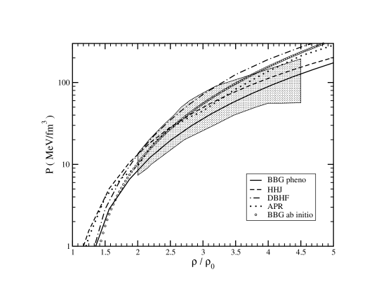
The variational EoS of Akmal et al. (1998), as well as the EoS derived from BHF together with phenomenological TBF, look in agreement with the phenomenological analysis, while the EoS from the DBHF calculations of van Dalen et al. (2005) is only marginally compatible, see also the paper by Klähn et al. (2006). The non–relativistic EoS calculated with BHF and “ab initio” TBF reported by Zuo et al. (2002) looks close to the BHF results with phenomenological TBF up to 2-3 time saturation density, giving further support to the phenomenological TBF, see also Zhou et al. (2006). However, at higher density it becomes too stiff and definitely falls outside the allowed region.
In turns out that also many phenomenological EoS do not pass this test (Klähn et al. 2006).
It has to be noticed that the flow values, and other observable quantities, in general do not depend only on the nuclear EoS, as embodied in the single particle potential, but also on the in–medium nucleon–nucleon collision cross section and on the effective mass (i.e. momentum dependence of the single particle potential). The extraction of meaningful information from the experiments requires a careful analysis and interpretation of the data. Other quantities which are related to the EoS are the rates of particle production, in particular and and their ratio. In fact the strange particle production is intimately related to the density reached during the collision and therefore to the nuclear matter compressibility. However in order to reach meaningful conclusions, it is necessary to have a reasonably good description of the behaviour of kaons in the nuclear medium at high density, which is not an easy task theoretically.
On the astrophysical side, as it is well known, each EoS for asymmetric matter gives rise to a definite relationship between the mass and radius of neutron stars (NS). This is because ordinary NS are bound by gravity and the solution of the Tolmann–Opennheimer–Volkoff (TOV) equation, based only on general relativity and the adopted EoS, provides the full density profile of the star. Unfortunately it is quite difficult to get from observation both the mass and the radius of a single NS, and up to now the accuracy, especially of the radius value, is not good enough to discriminate among different EoS. The quantity which has been mostly given attention is then the maximum mass of NS. The mass vs. radius plot has indeed a maximum value at the smaller radius, beyond which the star configuration is unstable towards collapse to a black hole. This maximum is characteristic of each EoS, and the observation of a NS with a mass larger than the predicted one would rule out the corresponding EoS. If one assumes that only nucleonic degrees of freedom are present inside the NS, then one can adopt the EoS discussed above. It turns out that BHF EoS give a maximum mass close to two solar masses, while the DBHF and variational ones a slightly larger value, around 2.2 – 2.3 solar masses. However, as already mentioned, the variational EoS of Akmal et al. (1998) becomes superluminal at high density, and actually the corrected one by Heiselberg and Hjorth–Jensen (1999) gives a maximum mass very close to 2 solar masses. Also the BHF EoS with the TBF by Zuo et al. (2002) gives a maximum mass larger than 2 (Zhou et al. 2004), but unfortunately this EoS becomes also superluminal already at relatively low density. From the astrophysical observations (mainly binary systems) the masses of NS were found, up to few years ago, mostly concentrated around 1.5 solar masses, the most precise one being 1.44 (Hulse and Taylor 1975). These values look compatible with the theoretical predictions. However, the situation for the maximum mass is by far much more complex. First of all it is likely that other degrees of freedom, besides the nucleonic ones, can appear inside a NS, in particular hyperonic matter. The BBG scheme has been extended to matter containing hyperons in several papers. If the most recent hyperon–nucleon and hyperon–hyperon interactions are used the maximum mass of NS drops to values below the observational limit (Schulze et al. 2006). There are two possibilities to overcome this failure in reproducing the observational constraint. The hyperon–nucleon and hyperon–hyperon interactions are poorly known from laboratory experiments, which presently are able to provide only few data points to be fitted. Different interactions, still compatible with phenomenology, could be able to produce a stiffer EoS at high density and consequently larger mass values. Another possibility is the appearance of other degrees of freedom, in particular the transition to quark matter could occur in the core of NS. This possibility has been studied extensively by many authors and indeed it has been found that the onset of the deconfined phase is able to increase the maximum mass to values compatible with the observational limit and ranging from 1.5 to 1.8 solar masses. These results have been obtained within simple quark matter models, like the MIT bag model, the Color Dielectric Model and the Nambu–Jona Lasinio model, with the possible inclusion of color superconductivity (Drago et al. 2005). If perturbative–like corrections to the simple MIT model are introduced, masses up to about 2 can be obtained (Alford et al. 2005). In any case, all that shows clearly the great relevance of the nowadays standard observations on NS to our knowledge of the high density nuclear EoS. The astrophysical observations are able to rule out definite EoS or put constraints on them.
As a final remark on this subject one has to mention the recent claims of the observation of NS with mass definitely larger than 2 (Nice et al. 2005, Özel 2006). If confirmed, these observations would put serious constraints on the nuclear EoS and would point to an additional repulsion which should be present at high density, i.e. a larger stiffness of the quark matter EoS. It has to be stressed that the nuclear EoS appropriate to NS cannot be directly applied to heavy ion collisions. The NS matter is in beta equilibrium and the strange content is determined by chemical equilibrium, which cannot be established during the collision time of heavy ions. In fact the hyperon multiplicity in heavy ion collisions is much smaller than one and no strange matter can be actually formed. Furthermore, the asymmetry of NS matter is much larger than the values reachable in laboratory experiments. Of course a good microscopic theory must be able to connect the two different physical situations within the same many–body scheme, which is one of the main challenges of nuclear physics.
11 Symmetry energy above saturation
At sub–saturation density the symmetry energy of nuclear matter seems to be under control from the theoretical point of view, since the different microscopic calculations agree among each other and the results look only marginally dependent on the adopted nuclear interaction. The symmetry energies calculated within the BBG scheme (Baldo et al. 2004), for different NN interactions (TBF have a negligible effect) are in agreement with each other and are reasonably well reproduced by some of the most used phenomenological Skyrme forces. Variational or DBHF calculations give very similar results. The approximate agreement of phenomenological calculations with the microscopic ones does not hold for all Skyrme forces, as shown e.g. by Chen et al. (2006), and a wide spread of values is actually found below saturation. The microscopic symmetry energy below saturation density can be approximately described by
where is the saturation density. Notice that the exponent is close to the one for a free Fermi gas (of course the absolute values are quite different by approximately a factor 2).
The symmetry energy at density above saturation can be studied with heavy ion reactions in central or semi–central collisions where nuclear matter can be compressed. Particle emissions and productions are among the processes which have been widely used to this purpose. Generally speaking the signal coming from these studies are weak because several competing effects are very often present at the same time and they largely cancel out among each other. In the paper by Ferini et al. (2006) the ratio between and rates and between and has been studied through simulations of central collisions in the energy range 0.8 – 1.8 GeV. These ratios seem to be dependent on the strength of the isovector part of the single particle potentials, but the dependence is not so strong, due to the compensation between symmetry potential effects and threshold effects. In any case it has to be stressed that the behaviour of mesons, or even mesons, in nuclear matter is a complex many–body problem, which complicates the interpretation of the experimental data.
To this respect one has to notice that it was suggested by Li et al. (1997) that in NS the onset of a kaon condensate could be possible. This can happen due to the steep increase inside the star of the electron chemical potential which can finally equal the in–medium mass of mass. Since this condensate produces a substantial softening of the EoS, the NS maximum mass turns out to be limited to about 1.5 solar masses. The possibility of kaon condensation was re–examined recently by Li et al (2006a). In any case, this value looks in contradiction with the latest observational data and shows once more the great value of the astrophysical studies on NS for our knowledge of dense nuclear matter.
Another process in NS which is sensitive to symmetry energy is cooling. The main mechanism of cooling is the direct Urca (DU) process
where neutrinos and antineutrinos escape from the star, cooling the object with a time scale of the order of million years. Since the chemical potentials of neutrons and protons are quite different because of the large asymmetry of the NS matter, the conservation of energy and momenta forbid these reactions when the percentage of protons is below 14% (when muons are also included). The percentage of protons is directly determined by the symmetry energy, and therefore the density at which the threshold for DU occurs is directly determined by the density dependence of the symmetry energy. At density above saturation this threshold can be different for different EoS. In some case, as for the EoS of Akmal et al. (1998), it is practically absent up to almost the central density of NS, even for the largest masses. In this case other processes, like the indirect Urca process, are the dominant cooling mechanism, which are however much less efficient than the DU process. Models of NS which do not include the DU process are only marginally successful in reproducing cooling data on NS (Yakovlev and Pethick 2004). If the DU threshold is at too “low” density, the cooling process can be too fast, even with the inclusion of nuclear matter pairing (Klähn 2006), which hinders the DU process. This is what occurs for the EoS derived from the DBHF method, whose symmetry energy rises steeply with density. The EoS from BHF, with the inclusion of phenomenological TBF, give a threshold density for DU process intermediate between these two cases and seem to be compatible with cooling data. For EoS with a similar behaviour of the symmetry energy the scenario of NS cooling involves a slow cooling for low masses and a fast one for the higher masses. Of course a more detailed description of NS cooling requires the many–body treatment of the different processes which can contribute (Blaschke et al. 2004). Finally, the possible onset of quark matter could again change the whole cooling scenario, which has then to be reconsidered, but the above general considerations can be still applied.
12 Conclusions
In this topical review we have presented the microscopic many–body theories, developed along the years, on the nuclear Equation of State, where only nucleonic degrees of freedom are considered. The results of different approaches have been critically compared, both at the formal and the numerical levels, with special emphasis on the high baryon density regime. The non–relativistic Bethe–Brueckner–Goldstone and variational methods are in fair agreement up to 5–6 times saturation density. When three–body forces are introduced, as required by phenomenology, some discrepancy appears for symmetric nuclear matter above 0.6 fm-3. The dependence of the results on the adopted realistic two–body forces and on the choice of the three–body forces has been analyzed in detail. It is found that a very precise reproduction of data on three– and four–body nuclear systems, as well as of the nuclear matter saturation point, is too demanding for the present day nuclear force models. In particular, if a very accurate description of few body systems is achieved by a suitable off–shell adjustment of the two–body forces, i.e. by introducing a non–local component, then the saturation point cannot be reproduced with a reasonable precision. However, local forces with phenomenological three–body forces are able to give an approximate reproduction both of the properties of few–body systems and of the nuclear matter saturation point, with a discrepancy on the binding energy per particle below 200–300 KeV.
The relativistic Dirac–Brueckner approach, as applied to nuclear matter, gives an Equation of State above saturation which is stiffer than the non–relativistic approaches. Some ambiguities related to the three–dimensional reduction of the fully relativistic two–body scattering matrix in the medium have still to be resolved.
We have then briefly reviewed the observational data on neutron stars and the experimental results on heavy ion collisions at intermediate and relativistic energies that could constrain the nuclear Equation of State at high baryon density. The EoS of the relativistic Dirac–Brueckner approach seems to present some discrepancies in comparison with constraints coming form heavy ion collisions and neutron stars data. The microscopic non–relativistic EoS turn out to be compatible with the phenomenological constraints available up to now. It looks likely that future developments in astrophysical observations and in laboratory experiments on heavy ion collisions will further constrain the nuclear EoS and give further hints on our knowledge of the fundamental processes which determine the behaviour of nuclear matter at high baryon density.
References
References
- [1]
- [2] [] Akmal A, Pandharipande V R and Ravenhall D G 1998, Phys. Rev. C58 1804.
- [3] [] Alford M, Braby M, Paris M and Reddy S 2005, ApJ 629 969.
- [4] [] Baldo M 1999 Nuclear Methods and the Nuclear Equation of State,Chapter 1, International Review of Nuclear Physics vol 8 (World Scientific) Baldo M Ed.
- [5] [] Baldo M, Giansiracusa G, Lombardo U and Song H Q 2000, Phys. Lett. B 473 1.
- [6] [] Baldo M, Fiasconaro A, Giansiracusa G, Lombardo U and Song H Q 2001, Phys. Rev. C 65 017303.
- [7] [] Baldo M, Maieron C, Schuck P and Viñas X 2004, Nucl. Phys. A 736 241.
- [8] [] Baldo M and Maieron C 2005, Phys. Rev. C 72 034005.
- [9] [] Bethe H A, Brandow B H and Petschek A G, 1962, Phys. Rev. 129 225.
- [10] [] Blaschke D, Grigorian H and Voskresensky D N 2004, Astron. Astrophys. 424 979.
- [11] [] Brockmann R and Machleidt R 1999, Nuclear Methods and the Nuclear Equation of State,Chapter 2, International Review of Nuclear Physics vol 8 (World Scientific) Baldo M Ed.
- [12] [] Brown G E, Weise W, Baym G and Speth J 1987, Comm. Nucl. Part. Phys. 17 39.
- [13] [] Chen L–W, Ko C M and Li B–A 2006, nucl-th/0610057.
- [14] [] Coester F, Cohen S, Day B D, and Vincent C M 1970, Phys. Rev. C 1 769.
- [15] [] Danielewicz P, Lacey R and Linch W G 2002, Science 298 1592.
- [16] [] Day B D 1981, Phys. Rev. C 24 1203.
- [17] [] Day B D 1983, Brueckner–Bethe Calculations of Nuclear Matter, Proceedings of the School E. Fermi, Varenna 1981, Course LXXIX, ed. A. Molinari, (Editrice Compositori, Bologna), p. 1–72.
- [18] [] Doleschall P and Borbely I 2000, Phys. Rev. C 62 054004.
- [19] [] Doleschall P, Borbely I, Papp Z and Plessas W 2003, Phys. Rev. C 67 064005.
- [20] [] Doleschall P 2004, Phys. Rev. C 69 054001.
- [21] [] Drago A, Lavagno A and Pagliara G 2005, Nucl. Phys. Proc. Supplements B 138 522.
- [22] [] Fadeev L D 1965, Mathematical Aspects of the Three-Body Problem in Quantum Scattering Theory, Davey, New York.
- [23] [] Fantoni S and Rosati S 1974, Nuovo Cimento A 20 179.
- [24] [] Ferini G, Gaitanos T, Colonna M, Di Toro M and Wolter H H 2006, Phys. Rev. Lett. 97 202301.
- [25] []Fetter A L and Walecka J D 1971 Quantum Theory of Many Particle Physics (New York : McGraw-Hill).
- [26] [] Gell-Mann M and Low L, 1951 Phys. Rev.84 350.
- [27] [] Goldstone J 1957 Proc. Roy. Soc. (London) A 239 267; Bethe H A and Goldstone J 1957 Proc. Roy. Soc. (London) A 238 551.
- [28] [] Grangé P, Lejeune A, Martzolff M and Mathiot J-F 1989, Phys. Rev. C 40 1040.
- [29] [] Gross–Boelting T, Fuchs Ch and Faessler A 1999, Nucl. Phys. A 648 105.
- [30] [] Heiselberg H and M. Hjorth-Jensen M 1999, Astrophys. J. 525 L45.
- [31] [] Hulse R H and J.H. Taylor J H 1975, Astrophys. J. 195 L51.
- [32] [] Jackson A D, Landé A and Smith R A 1982, Phys. Rep. 86 55.
- [33] [] Klähn T, Blaschke D, Sandin F, Fuchs Ch, Faessler A, Grigorian H, Ropke G and Trümper J 2006, nucl-th/0609067.
- [34] [] Kowalski K, Dean D J, Hjorth-Jensen M, Papenbrock T and Piecuch P 2004, Phys. Rev. Lett. 92 132501.
- [35] [] Dean D J and Hjorth-Jensen M 2004, Phys. Rev. C 69 054320.
- [36] [] Kümmel H and Lührmann H 1972, Nucl. Phys. A 191 525.
- [37] [] Kümmel H, Lührmann H K and Zabolitzky J G 1978, Phys. Rep. 36 1.
- [38] [] Lagaris I E and Pandharipande V R 1980, Nucl. Phys. A 334 217.
- [39] [] Lagaris I E and Pandharipande V R 1981, Nucl. Phys. A 359 349.
- [40] [] Lazauskas R and Carbonell J 2004, Phys. Rev. C 70 044002.
- [41] [] Li A, Burgio G F, Lombardo U and Zuo W 2006a, Phys. Rev. 74 055801.
- [42] [] Leeuwen J M J, Groeneveld J and de Boer J 1959, Physica 25 792.
- [43] []Li G Q, Lee C H and Brown G E 1997, Phys. Rev. Lett. bf 79 5214.
- [44] [] Li Z H, Lombardo U, Schulze H-J, Zuo W, Chen L W and Ma H R 2006b, Phys. Rev. C 74 047304.
- [45] [] Lührmann K H 1975, Ann. Phys. 103 253.
- [46] [] Machleidt R 1989, Advances in Nuclear Physics Vol. 19 pp. 189, Plenum Press.
- [47] [] Machleidt R 2001, Phys. Rev. C 63 024001.
- [48] [] Morales J, Jr., Pandharipande V R and Ravenhall 2002, Phys. Rev. C 66 054308.
- [49] [] Navarro J, Guardiola R and Moliner I 2002, Introduction to Modern Methods of Quantum Many-Body Theory and their Applications, Eds. Fabrocini A, Fantoni S and Krotscheck E, World Scientific, Series on Advances in Many-Body Theory, Vol. 7.
- [50] [] Nice D J et al. 2005, ApJ 634 1242.
- [51] [] Özel F 2006, Nature 441 1115 ; astro-ph/0605106.
- [52] [] Newton R G 1966, Scattering Theory of Waves and Particles, Mc-Graw Hill.
- [53] [] Pandharipande V R and Wiringa R B 1979, Rev. Mod. Phys. 51 821.
- [54] [] Rajaraman R and Bethe, H A 1967, Rev. Mod. Phys. 39 745.
- [55] [] Schulze H–J, Polls A, Ramos A and Vidaña I 2006, Phys. Rev. C 73, 058801.
- [56] [] Stocks V G J,Klomp R A M, Terheggen C P F de Swart J J 1994, Phys. Rev. C 49 2950.
- [57] [] Ter Haar B and Malfliet R 1987, Phys. Rep. 149, 207.
- [58] [] van Dalen E N E, Fuchs Ch and Faessler A 2005, Phys. Rev. C72 065803.
- [59] [] Wiringa R B, Stoks V G J and Schiavilla R 1995, Phys. Rev. C 51, 38.
- [60] [] Wiringa R B, Smith R A and Ainsworth T L 1984, Phys. Rev. C 29, 1207.
- [61] [] Yakovlev D G and Pethick C J 2004, Ann. Rev. Astron. Astrophys. 42 169 (2004).
- [62] [] Zhou X R, Burgio F G, Lombardo U, Schulze H–J and Zuo W 2004, Phys. Rev. C 69 018801.
- [63] [] Zuo W, Lejeune A, Lombardo U and Mathiot J-F 2002, Nucl. Phys. A 706 418 ; EPJA 14 469.