Bjorken expansion with gradual freeze out

Abstract

The freeze out of the expanding systems, created in relativistic heavy ion collisions, will be discussed. We combine kinetic freeze out equations with Bjorken type system expansion into a unified model. Such a model is a more physical generalization of the earlier simplified non-expanding freeze out models. We shall see that the basic freeze out features, pointed out in the earlier works, are not smeared out by the expansion.

1 Model for the simultaneously expanding and freezing out fireball

In this paper we present a simple freeze out (FO) model, which describes the FO of particles from a Bjorken expanding fireball [1]. The important feature of the proposed scenario is that physical freeze out is completely finished in a finite time, which can be varied from $0$ (FO hypersurface) to $\infty$. In the other words our FO happens in a layer, i.e. in a domain restricted by two parallel hypersurfaces $\tau=\tau_{1}$ and $\tau=\tau_{1}+L$, where $\tau$ is the proper time variable and $L$ is the maximal duration of the FO process.
The present model simultaneously describes the gradual FO and the expansion of the system, and thus it is a more realistic extension of the oversimplified FO models, which did not include system expansion [2, 3, 4, 5]. In Ref. [3] authors have also adopted kinetic gradual FO model to Bjorken geometry, but combined it with Bjorken expansion on the consequent, not on the parallel basis: system expands according to Bjorken hydro scenario, but when it reaches beginning of the FO process system stops expansion and gradually freezes out in a fixed volume. It was shown in [3] that although such a model allows to obtain analytical results, it is not physical, the simultaneous modeling of expansion and freeze out is required in order to avoid decreasing of the total entropy. And now we propose such a generalized model [9].
We start with introducing two components of the distribution function, $f$: the interacting, $f^{i}$, and the frozen out, $f^{f}$ ones, ($f=f^{i}+f^{f}$), then, correspondingly we will have two components of the energy density and baryon density. Details of the derivation can be found in Ref. [9] and here we only give the final coupled system of equations for interacting and free components describing the change in the particle density and energy density:

$$\frac{de^{i}}{d\tau}=-\frac{e^{i}+P^{i}}{\tau}-\frac{e^{i}}{\tau_{FO}}\frac{L}{L+\tau_{1}-\tau}\,;\quad\frac{dn^{i}}{d\tau}=-\frac{n^{i}}{\tau}-\frac{n^{i}}{\tau_{FO}}\frac{L}{L+\tau_{1}-\tau}\,,$$ (1)

$$\frac{de^{f}}{d\tau}=-\frac{e^{f}}{\tau}+\frac{e^{i}}{\tau_{FO}}\frac{L}{L+\tau_{1}-\tau}\,;\quad\frac{dn^{f}}{d\tau}=-\frac{n^{f}}{\tau}+\frac{n^{i}}{\tau_{FO}}\frac{L}{L+\tau_{1}-\tau}\,.$$ (2)

All together we have the following simple model describing the evolution of the fireball created in relativistic heavy ion collision.
Initial state: $\tau=\tau_{0}$  ,

$$e(\tau)=e_{0}\,,\quad n(\tau)=n_{0}\,.$$ (3)

Phase I, Pure Bjorken hydrodynamics: $\tau_{0}\leq\tau\leq\tau_{1}$  ,

$$e(\tau)=e_{0}\left(\frac{\tau_{0}}{\tau}\right)^{1+c_{0}^{2}}\,,\quad n(\tau)=n_{0}\left(\frac{\tau_{0}}{\tau}\right)\,,$$ (4)

where $P=c_{0}^{2}e$ is the equation of state (EOS).
Phase II, Bjorken expansion and gradual FO: $\tau_{1}\leq\tau\leq\tau_{1}+L$   ,

$$e^{i}(\tau)=e_{0}\left(\frac{\tau_{0}}{\tau}\right)^{1+c_{0}^{2}}\left(\frac{L+\tau_{1}-\tau}{L}\right)^{L/\tau_{FO}},\,n^{i}(\tau)=n_{0}\left(\frac{\tau_{0}}{\tau}\right)\left(\frac{L+\tau_{1}-\tau}{L}\right)^{L/\tau_{FO}}.$$ (5)

The difference with respect to the pure Bjorken solution eqs. (4) is the multiplier describing the gradual FO of the system. We also see that the interacting component will vanish when we reach the end of the FO layer, i.e. $\tau\rightarrow L+\tau_{1}$.

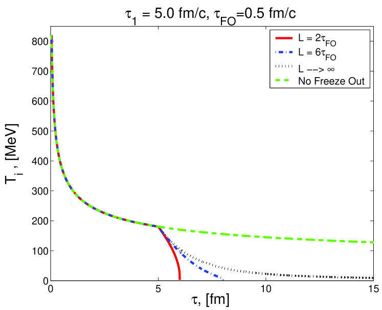
Figure 1: Evolution of temperature of the interacting matter for different FO layers. $T_{i}(\tau_{0}=0.05\ fm)=820\ MeV$, $T_{FO}=180\ MeV$. ”No Freeze Out” means that we used standard Bjorken hydrodynamics even in phase II.

Knowing $e^{i}(\tau)$ and equation of state (EoS) we can calculate the temperature of the interacting component, $T_{i}(\tau)$, as a function of the proper time. Due to symmetry of the system, $u_{i}^{\mu}(\tau)=u^{\mu}(\tau_{0})=(1,0,0,0)$. Thus, we have complete knowledge about the evolution of the interacting component, $f^{i}(\tau)$, which is a thermal distribution with given $T_{i}(\tau)$, $n^{i}(\tau)$, $u_{i}^{\mu}(\tau)$.
However, what we have to calculate is the free component, which is the source of the observables. Eqs. (2) give us the evolution of the $e_{f}$ and $n_{f}$, and one can easily check that these two equations are equivalent with the following equation for the free component:

$$\frac{df^{f}}{d\tau}=-\frac{f^{f}}{\tau}+\frac{f^{i}}{\tau_{FO}}\left(\frac{L}{L+\tau_{1}-\tau}\right)\,.$$ (6)

The measured post FO spectra are given by $f^{f}(L+\tau_{1})$.

2 Results from the model

Aiming for a qualitative illustration of the FO process we show below the results for the ideal massive pion gas with Jüttner equilibrated distribution [10]:

$$f^{i}(\tau,\mathbf{p})=\frac{g}{(2\pi)^{3}}e^{-\sqrt{|\mathbf{p}|^{2}+m_{\pi}^{2}}/T_{i}(\tau)}\,,$$ (7)

where the degeneracy of pion is $g=3$, while the baryon chemical potential in case of pions is zero.
Contrary to the illustrative example in [9] here we do not neglect the pion mass. During FO the temperature of the interacting component decreases to zero, so at late stages of the FO process this new calculation is better justified. We will see below that $T_{i}$ falls below $m_{\pi}$ quite soon, and so the Jüttner distribution is a good approximation of the proper Bose pion distribution.
For our system we have the following EoS:

$$e^{i}=\frac{3g}{2\pi^{2}}m^{2}T_{i}^{2}K_{2}(a)+\frac{g}{2\pi^{2}}m^{3}T_{i}K_{1}(a)\,,\quad P^{i}=\frac{g}{2\pi^{2}}m^{2}T_{i}^{2}K_{2}(a)\,,$$ (8)

where $K_{n}$ is Bessel function of the second kind, and $a=m/T_{i}$.

The first eq. of system (1), gives the following equation for the evolution of the temperature of the interacting component:

$$\frac{dT_{i}}{d\tau}=-\frac{T_{i}}{\tau}\frac{4T_{i}^{2}K_{2}(a)+mT_{i}K_{1}(a)}{12T_{i}^{2}K_{2}(a)+5mT_{i}K_{1}(a)+m^{2}K_{0}(a)}$$

$$-\frac{T_{i}}{\tau_{FO}}\left(\frac{L}{L+\tau_{1}-\tau}\right)\frac{3T_{i}^{2}K_{2}(a)+mT_{i}K_{1}(a)}{12T_{i}^{2}K_{2}(a)+5mT_{i}K_{1}(a)+m^{2}K_{0}(a)}\,.$$ (9)

Furthermore, we have used the following values of the parameters: $\eta_{R}=4.38$, $A_{xy}=\pi R_{Au}^{2}$, where $R_{Au}=7.685$ fm is the $Au$ radius, $\tau_{0}=0.05\ fm$, $T_{i}(\tau_{0})=820\ MeV$, $\tau_{1}=5\ fm$, what leads to $T_{i}(\tau_{1})=T_{FO}=180\ MeV$, and $\tau_{FO}=0.5\ fm$. During the pure Bjorken case the evolution of the temperature is govern by a simplified eq. (9), without the second freeze out term on r.h.s.

In Fig. 1 we present the evolution of the temperature of the interacting matter, $T_{i}(\tau)$, for different values of FO time $L$.

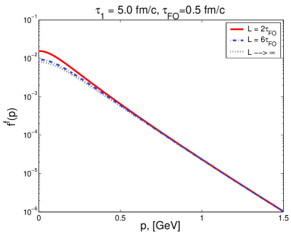
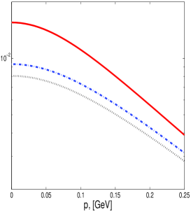
Figure 2: Final post FO distribution for different FO layers as a function of the momentum in the FO direction, $p=p^{x}$ in our case ($p^{y}=p^{z}=0$). The initial conditions are specified in the text.

As it was already shown in Ref.[3, 5], the final post FO particle distributions, shown on Fig. 2, are non-equilibrated distributions, which deviate from thermal ones particularly in the low momentum region. By introducing and varying the thickness of the FO layer, $L$, we are strongly affecting the evolution of the interacting component, see Fig. 1, but the final post FO distribution shows strong universality: for the FO layers with a thickness of several $\tau_{FO}$ post FO distribution already looks very close to that for an infinitely long FO calculations, see Fig. 2 left plot. Differences can be observed only for the very small momenta, as shown in Fig. 2 right plot. So, the inclusion of the expansion into our consideration does not smear out this very important feature of the gradual FO.
It is important to always check the non-decreasing entropy condition [9, 11] to see whether such a process is physically possible. Figs. 3 present the evolution of the total entropy, $S(\tau)$, calculated based on the full distribution function, $f(\mathbf{p})=f^{i}(\mathbf{p})+f^{f}(\mathbf{p})$:

$$s(\tau)=\int d^{3}pf(\tau)\left[1-\ln\left(\frac{(2\pi)^{3}}{g}f(\tau)\right)\right]\,,\quad S(\tau)=s(\tau)V(\tau)\,.$$ (10)

During pure Bjorken phase total entropy remains constant, as expected, but during phase II it constantly increases until FO is finished.

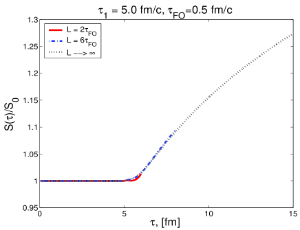
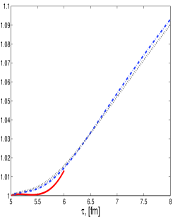
Figure 3: Evolution of the total entropy for different FO layers. The initial conditions are specified in the text.

From this figure we can make an important conclusion, that gradual freeze out produces entropy. For the late stages of the FO this can be approximated analytically.

$$\frac{ds(\tau)}{d\tau}=\int d^{3}p\frac{df(\tau)}{d\tau}\left[1-\ln\left(\frac{(2\pi)^{3}}{g}f(\tau)\right)\right]-\int d^{3}p\frac{df(\tau)}{d\tau}\,,$$ (11)

At the late stages of the FO contribution of the interacting component can be neglected, so $f\approx f^{f}$, and, from eq. (6), $\frac{df^{f}}{d\tau}\approx-\frac{f^{f}}{\tau}$. So for the late stages of the reaction we have the following equation for the entropy evolution:

$$\frac{ds(\tau)}{d\tau}\approx-\frac{s(\tau)}{\tau}+\frac{n^{f}(\tau)}{\tau}\,.$$ (12)

And since in the Bjorken geometry $V(\tau)\sim\tau$ we obtain:

$$\frac{dS}{d\tau}=\frac{d\left(sV\right)}{d\tau}\approx-\frac{sV}{\tau}+\frac{n^{f}V}{\tau}+\frac{sV}{\tau}=\frac{N_{f}}{\tau}\,,$$ (13)

where $N_{f}$ is total number of frozen out particles. Thus, we see that total entropy increases during the simultaneous expansion and gradual FO, and at the very end of the FO process it increases logarithmically.

3 Conclusions

In this paper we presented a gradual FO model including a Bjorken like expansion, being an extension to the older versions [2, 3, 4, 5], which allowed us to study FO in a layer of any thickness, $L$, from $0$ to $\infty$. Another important feature of the proposed model is that it connects the pre FO hydrodynamical quantities, like energy density, $e$, baryon density, $n$, with post FO distribution function in a relatively simple way, and furthermore allows analytical analysis for simple systems, like massless pion gas [9].
The results show that the inclusion of the expansion into FO model, although strongly affects the evolution of the interacting component, does not smear out the universality of the final post FO distribution, observed already in Refs. [3, 4, 5].
Another important conclusion of this work, stressing once again the importance to always check the non-decreasing entropy condition [9, 11], is that long gradual freeze out may produce substantial amount of entropy, as shown on Fig. 3.

References

- [1] J. D. Bjorken, Phys. Rev. D 27 (1983) 140.
- [2] Cs. Anderlik et al., Phys. Rev. C59 (1999) 388; Phys. Lett. B459 (1999) 33; V.K. Magas et al., Nucl. Phys. A661 (1999) 596; Heavy Ion Phys. 9 (1999) 193.
- [3] V.K. Magas et al., Eur. Phys. J. C30 (2003) 255.
- [4] E. Molnár et al., Phys. Rev. C74 (2006) 024907, V.K. Magas et al., nucl-th/0510066.
- [5] E. Molnár et al., nucl-th/0503048.
- [6] V.K. Magas et al., Nucl. Phys. A749 (2005) 202; L.P. Csernai et al., hep-ph/0406082; Eur. Phys. J. A25 (2005) 65.
- [7] L.P. Csernai et al., hep-ph/0401005; E. Molnár et al., nucl-th/0510062.
- [8] K. J. Eskola, K. Kajantie and P. V. Ruuskanen, Eur. Phys. J. C 1 (1998) 627.
- [9] V.K. Magas, L.P. Csernai, E. Molnar, nucl-th/0702069; V.K. Magas, talk at the International Workshops on Critical Point and Onset of Deconfinement, Florence, Italy, July 3-6, 2006.
- [10] F. Jüttner, Ann. Phys. Chem. 34, 856 (1911).
- [11] Cs. Anderlik et al., Phys. Rev. C59 (1999) 3309.