Particle number fluctuations in nuclear collisions
within excluded volume hadron gas model

Abstract

The multiplicity fluctuations are studied in the van der Waals excluded volume hadron-resonance gas model. The calculations are done in the grand canonical ensemble within the Boltzmann statistics approximation. The scaled variances for positive, negative and all charged hadrons are calculated along the chemical freeze-out line of nucleus-nucleus collisions at different collision energies. The multiplicity fluctuations are found to be suppressed in the van der Waals gas. The numerical calculations are presented for two values of hard-core hadron radius, $r=0.3$ fm and 0.5 fm, as well as for the upper limit of the excluded volume suppression effects.

I Introduction

During last decades statistical models of strong interactions have served as an important tool to investigate high energy nuclear collisions. The main object of the study have been the mean multiplicities of produced hadrons (see e.g. Refs. FOC ; FOP ; pbm ). Only recently, due to a rapid development of experimental techniques, first measurements of fluctuations of particle multiplicities fluc-mult and transverse momenta fluc-pT were performed. The study of event-by-event fluctuations in nucleus-nucleus collisions (see e.g., reviews fluc1 ) is motivated by expectations of anomalies in the vicinity of the onset of deconfinement ood and in the case when the expanding system goes through the transition line between the quark-gluon plasma and the hadron gas fluc2 . Furthermore, it is expected that a critical point of strongly interacting matter may be signaled by a characteristic pattern in fluctuations fluc3 .

A convenient measure of the particle number fluctuations is the scaled variance, $\omega\equiv Var(N)/\langle N\rangle$, defined in terms of the mean value, $\langle N\rangle$, and variance, $Var(N)\equiv\langle N^{2}\rangle-\langle N\rangle^{2}$. The scaled variance equals to 1 for the ideal Boltzmann gas in the grand canonical ensemble (GCE). The deviations of $\omega$ from unity in the hadron-resonance gas (HG) come due to Bose and Fermi statistics, resonance decays (see, e.g., Ref. fluc1 ), and exactly enforced conservations laws CE ; res_CE ; res_MCE . Previous study res_MCE has shown a rather rapid convergence of the scaled variances to asymptotic values. Finite system size effects can therefore be ignored for central collisions of heavy nuclei.

The effect of Bose and Fermi statistics can be seen in the primordial (before resonance decay) values of the scaled variances in the GCE (see, e.g., Ref. res_CE ). For chemical freeze-out at low collision energies (small temperature $T$ and large baryonic chemical potential $\mu_{B}$) most charged particles are protons. Fermi statistics then lead to a suppression of positively charged and all charged particle number fluctuations, $\omega_{+}\cong\omega_{ch}=0.98\div 1$. At high collision energies (large $T$ and small $\mu_{B}$) most charged particles are pions. Thus, Bose statistics dominates and leads to the enhancement of particle number fluctuations, $\omega_{\pm}\cong\omega_{ch}=1.05\div 1.06$. These numbers demonstrate that the effects of quantum statistics are small at the chemical freeze-out.

Resonance decay in the GCE and CE lead to the enhancement of particle number fluctuations. At high collision energies (the largest SPS energy and above) the GCE calculations give the following final (after resonance decay) values, $\omega_{\pm}\cong 1.1$ and $\omega_{ch}\cong 1.6$  res_CE .

There is a qualitative difference in the properties of the mean multiplicity and the scaled variance of multiplicity distribution in statistical models. In the case of the mean multiplicity results obtained with the GCE, canonical ensemble (CE), and micro-canonical ensemble (MCE) approach each other in the large volume limit (this reflects the thermodynamical equivalence of statistical ensembles). It was recently found CE ; res_CE ; res_MCE that corresponding results for the scaled variance are different in different ensembles, and, thus, the scaled variance is sensitive to conservation laws obeyed by a statistical system. The differences are preserved in the thermodynamic limit. The global conservation laws imposed on each microscopic state of the statistical system lead to the suppression of particle number fluctuations. At large $T$ and small $\mu_{B}$ (high collision energies) the final state scaled variances behave in the CE as, $\omega_{\pm}\cong 0.8$ and $\omega_{ch}\cong 1.6$ res_CE , and in the MCE as, $\omega_{\pm}\cong 0.3$ and $\omega_{ch}\cong 0.6$  res_MCE .

It has been found that the fluctuations in the number of nucleon participants give a large contribution to hadron multiplicity fluctuations in peripheral A+A collisions. Thus ideally a comparison between data and predictions of statistical models should be performed for results which correspond to collisions with a fixed number of nucleon participants. This can approximately be achieved by selecting only the most central A+A collisions (see Ref. Voka ; MGMG for details). The conditions for the centrality selection in the study of fluctuations should thus be much more stringent than in the multiplicity measurements. To minimize the contributions from the participant number fluctuations, one should restrict the analysis to the 1% most central A+A collisions selected by the number of projectile spectators (see Refs. res_MCE ; NA49 ). In this sample both the fluctuations of the number of participating nucleons and the resulting enhancement of multiplicity fluctuations should not exceed a few %.

Usually the ideal HG gas is used for the particle multiplicity calculations. The extension of the ideal gas picture based on the van der Waals (VDW) excluded volume procedure have been suggested in Refs. vdw ; vdw1 ; crit to phenomenologically take into account repulsive interactions between hadrons. This leads to the suppression of hadron number densities and energy density. In the present paper we study the effect of the VDW excluded volume on the multiplicity fluctuations. The particle number ratios are independent of the proper volume parameter, if it is the same for all hadron species. Thus, a rescaling of the total volume $V$ leads to exactly the same hadron yields as those in the ideal HG. In the present paper it is demonstrated that the multiplicity fluctuations are suppressed in the VDW gas. This suppression is qualitatively different from that of particle yields. In contrast to average multiplicities, the suppression of multiplicity fluctuations can not be removed by rescaling of the total volume of the system.

In the present study we restrict ourself to the GCE calculations within the Boltzmann statistics approximation. The paper is organized as follows. In Section II the ideal HG model is presented. In Section III the one-component VDW gas is used to calculate the average multiplicity and the scaled variance. These results are extended to the multi-component VDW gas in Section IV. Both primordial and final state (after resonance decay) hadron yields and their fluctuations are considered. In Section V the scaled variance of negative, positive and all charged hadrons is calculated along the chemical freeze-out line. This gives the VDW HG predictions for fluctuations of hadron multiplicities in central A+A collisions at different collision energies from SIS to LHC. A summary, presented in Section VI, closes the paper.

II Ideal Hadron-resonance Gas

The partition function of the ideal Boltzmann HG in the GCE has the form:

$$Z_{id}~{}=~{}\exp\left[\sum_{j}V~{}\phi_{j}~{}\right]~{},$$ (1)

where:

$$\phi_{j}~{}\equiv~{}\lambda_{j}~{}\frac{g_{j}}{2\pi^{2}}~{}~{}\int_{0}^{\infty}k^{2}dk~{}\exp\left[-~{}\frac{(k^{2}~{}+~{}m_{j}^{2})^{1/2}}{T}\right]=~{}\lambda_{j}~{}\frac{g_{j}}{2\pi^{2}}~{}m_{j}^{2}~{}T~{}K_{2}\left(\frac{m_{j}}{T}\right)~{}.$$ (2)

In Eqs. (1,2), $\lambda_{j}=\exp\left(\mu_{j}/T\right)$ is the particle specific fugacity, $g_{j}$ the degeneracy of $j$th particle species, $m_{j}$ the particle mass, and $\mu_{j}=b_{j}\mu_{B}+s_{j}\mu_{S}+q_{j}\mu_{Q}$ the chemical potential due to the $j$th particle internal quantum numbers $\left(b_{j},s_{j},q_{j}\right)$. The $j$-summation in Eq. (1) is taken over all hadron species. Global chemical potentials ($\mu_{B}$, $\mu_{S}$, $\mu_{Q}$) and temperature $T$ regulate the systems average charges (baryonic, strangeness, electrical) and energy densities. Finally, $V$ is the volume of the system and $K_{2}$ is the modified Hankel function.

II.1 Primordial Fluctuations

In the GCE the first two moments of the multiplicity distribution of $j$th particle are:

$$\langle N_{j}\rangle~{} =~{}\frac{1}{Z_{id}}\left(\lambda_{j}\frac{\partial}{\partial\lambda_{j}}\right)~{}Z_{id}~{}=~{}V~{}\phi_{j}~{},$$ (3)

$$\langle N_{j}^{2}\rangle~{} =~{}\frac{1}{Z_{id}}\left(\lambda_{j}\frac{\partial}{\partial\lambda_{j}}\right)^{2}~{}Z_{id}~{}=~{}\left(V\phi_{j}\right)^{2}~{}+~{}V\phi_{j}~{}.$$ (4)

Thus, $\phi_{j}$ is the $j$th hadron number density, $n_{j}^{id}$. The variance of the $j$th particle number distribution is:

$$\langle\left(\Delta N_{j}\right)^{2}\rangle~{}\equiv~{}\langle\left(N_{j}~{}-~{}\langle N_{j}\rangle\right)\rangle^{2}~{}=~{}\langle N_{j}^{2}\rangle-\langle N_{j}\rangle^{2}~{}=~{}\langle N_{j}\rangle~{},$$ (5)

and the scaled variance equals unity,

$$\omega_{j}~{}\equiv~{}\frac{\langle\left(\Delta N_{j}\right)^{2}\rangle}{\langle N_{j}\rangle}~{}=~{}1~{}.$$ (6)

For the average multiplicity and variance of, for example, positively charged primordial hadrons (i.e. before resonance decay) one obtains:

$$\langle N_{+}\rangle~{}=~{}\sum_{j,~{}q_{j}>0}\langle N_{j}\rangle~{},\qquad~{}\qquad~{}\langle\left(\Delta N_{+}\right)^{2}\rangle~{}=~{}\sum_{j,~{}q_{j}>0}~{}\sum_{k,~{}q_{k}>0}~{}\langle\Delta N_{j}\Delta N_{k}\rangle~{}.$$ (7)

The results for the negatively charged or all charged hadrons are similar to Eq. (7) with summation over negative charges, $q_{j}<0,~{}q_{k}<0$, or all non-zero charges, $q_{j}\neq 0,~{}q_{k}\neq 0$, respectively. For $j\neq k$, one finds,

$$\langle N_{j}N_{k}\rangle~{}=~{}\frac{1}{Z_{id}}\left[\left(\lambda_{j}\frac{\partial}{\partial\lambda_{j}}\right)~{}\left(\lambda_{k}\frac{\partial}{\partial\lambda_{k}}\right)\right]~{}Z_{id}~{}=~{}\langle N_{j}\rangle~{}\langle N_{k}\rangle~{},$$ (8)

and from Eqs. (5) and (8) it then follows,

$$\langle\Delta N_{j}\Delta N_{k}\rangle~{}=~{}\langle N_{j}N_{k}\rangle-\langle N_{j}\rangle~{}\langle N_{k}\rangle~{}=~{}\delta_{jk}~{}\langle N_{j}\rangle~{}.$$ (9)

From Eq. (9) one concludes that in the ideal HG the correlations between different particle species are absent in the GCE. Any particle number distribution in the ideal Boltzmann gas is Poissonian (for large average multiplicity this is equivalent to a Gaussian) and its scaled variance therefore equals unity. For example, the scaled variance for positively charged hadrons is,

$$\omega_{+}~{}=~{}\frac{\langle\left(\Delta N_{+}\right)^{2}\rangle}{\langle N_{+}\rangle}~{}=~{}1~{}.$$ (10)

This is also valid for negatively charged and all charged hadrons.

II.2 Final State Fluctuations

Final state yields and (co)variance have simple forms in the GCE Koch :

$$\langle N_{j}\rangle~{} =~{}\langle N_{j}^{*}\rangle~{}+~{}\sum_{R}~{}\langle N_{R}\rangle~{}\langle n_{j}\rangle_{R}~{},$$ (11)

$$\langle\Delta N_{j}\Delta N_{k}\rangle~{} =~{}\langle\left(\Delta N_{j}^{*}\right)^{2}\rangle~{}\delta_{jk}~{}+~{}\sum_{R}~{}\langle(\Delta N_{R})^{2}~{}\rangle\langle n_{j}\rangle_{R}\langle n_{k}\rangle_{R}~{}+~{}\sum_{R}~{}\langle N_{R}~{}\rangle\langle\Delta n_{j}\Delta n_{k}\rangle_{R}~{},$$ (12)

where $N_{j}^{*}$ is primordial $j$th hadron multiplicity, and:

$$\langle n_{j}\rangle_{R}~{} =~{}\sum_{r}~{}b_{r}^{R}~{}n_{j,R}^{r}~{},$$ (13)

$$\langle\Delta n_{j}\Delta n_{k}\rangle_{R}~{} =~{}\langle n_{j}n_{k}\rangle_{R}~{}-\langle n_{j}\rangle_{R}\langle n_{k}\rangle_{R}~{}=~{}\sum_{r}~{}b_{r}^{R}~{}n_{j,R}^{r}~{}n_{k,R}^{r}~{}-~{}\langle n_{j}\rangle_{R}\langle n_{k}\rangle_{R}~{},$$ (14)

$b_{r}^{R}$ is the branching ratio of the $r$th decay channel of $R$th resonance with normalization condition $\sum_{r}b_{r}^{R}=1$, while $n_{j,R}^{r}$ and $n_{k,R}^{r}$ are the respective multiplicities of particles of species $j$ and $k$ in $r$th decay channel of $R$th resonance. Generally, one finds enhancement of fluctuations due to resonance decay which leads to $\omega_{j}>1$ (valid in GCE and CE, see, e.g., Ref. res_CE ). The first term in the right hand side of Eq. (12) corresponds to fluctuation of $R$th resonance multiplicity and the second term appears due to the probabilistic character of resonance decay. For the Boltzmann gas discussed in this paper, it follows, $\langle(\Delta N_{R})^{2}\rangle=\langle N_{R}\rangle$, $\langle(\Delta N_{j})^{2}\rangle=\langle N_{j}^{*}\rangle$, and Eq. (12) simplifies to:

$$\langle\Delta N_{j}\Delta N_{k}\rangle~{}=~{}\langle N_{j}^{*}\rangle~{}\delta_{jk}~{}+~{}\sum_{R}~{}\langle N_{R}~{}\rangle\langle n_{j}n_{k}\rangle_{R}~{}.$$ (15)

From Eqs. (11) and (15) it immediately follows,

$$\omega_{j}~{}=~{}\frac{\langle N_{j}^{*}\rangle~{}~{}+~{}\sum_{R}~{}\langle N_{R}~{}\rangle\langle n_{j}^{2}\rangle_{R}}{\langle N_{j}^{*}\rangle~{}~{}+~{}\sum_{R}~{}\langle N_{R}~{}\rangle\langle n_{j}\rangle_{R}}~{}.$$ (16)

Thus, $\omega_{j}\geq 1$ as a consequence of the inequality $(n_{j,R}^{r})^{2}\geq n_{j,R}^{r}$ , i.e. the scaled variance of $j$th hadron exceeds 1 due to the presence of resonances decaying into more than one $j$th hadron. Using Eqs. (11) and (15) for average yields and correlators one finds from (7),

$$\omega_{+}~{}=~{}\frac{\sum_{j,~{}q_{j}>o}~{}[~{}\langle N_{j}^{*}\rangle~{}~{}+~{}\sum_{k,~{}q_{k}>0}\sum_{R}~{}\langle N_{R}~{}\rangle\langle n_{j}n_{k}\rangle_{R}~{}]}{\sum_{j,~{}q_{j}>o}~{}[~{}\langle N_{j}^{*}\rangle~{}~{}+~{}\sum_{R}~{}\langle N_{R}~{}\rangle\langle n_{j}\rangle_{R}~{}]}~{},$$ (17)

and similar expressions for final state $\omega_{-}$ and $\omega_{ch}$ with the summation over $q_{j}<0,~{}q_{k}<0$ and $q_{j}\neq 0,~{}q_{k}\neq 0$, respectively.

III One-Component VDW Gas

The VDW excluded volume procedure gives the GCE partition function of one component Boltzmann gas vdw :

$$Z(V,T,\mu_{j})~{}=~{}\sum_{N=0}^{\infty}~{}\frac{1}{N!}~{}\left[(V~{}-~{}v_{j}N)~{}\phi_{j}~{}\right]^{N}~{}\theta(V-v_{j}N)~{},$$ (18)

where $v_{j}$ is the proper volume of the $j$th particle. For the ‘hard sphere’ particles with radius $r_{j}$ the volume parameter $v_{j}$ equals the ‘hard-core particle volume’, $4\pi r_{j}^{3}/3$, multiplied by a factor of 4. A Laplace transform of Eq. (18) reads:

$$\widehat{Z}(s,T,\mu_{j})~{}\equiv~{}\int_{0}^{\infty}dV\exp(-sV)~{}Z(V,T,\mu_{j})~{}=~{}\sum_{N=0}^{\infty}~{}\frac{\phi_{j}^{N}}{N!}~{}\int_{v_{j}N}^{\infty}dV\exp(-sV)~{}\left(V~{}-~{}v_{j}N\right)^{N}~{}$$

$$=~{}\left[~{}s~{}-~{}\exp(-v_{j}s)~{}\phi_{j}\right]^{-1}~{}.$$ (19)

The system pressure is defined by the pole-singularity, $s^{*}$, of the function, $\widehat{Z}$ (III),

$$p~{}\equiv~{}\lim_{V\rightarrow\infty}~{}T~{}\frac{\ln Z}{V}~{}=~{}T~{}s^{*}~{},$$ (20)

and, thus, satisfies the following equation,

$$p~{}=~{}\exp\left(-~{}\frac{v_{j}~{}p}{T}\right)~{}T~{}\phi_{j}~{}.$$ (21)

For $v_{j}=0$, Eq.(21) is evidently reduced to the ideal gas result, $p_{id}=T\phi_{j}$. The average particle number in the VDW gas equals to:

$$\langle N_{j}\rangle~{}=~{}\frac{1}{Z(V,T,\mu_{j})}\left(\lambda_{j}\frac{\partial}{\partial\lambda_{j}}\right)~{}Z(V,T,\mu_{j})~{}=\frac{V}{T}~{}\lambda_{j}~{}\frac{\partial p}{\partial\lambda_{j}}~{}.$$ (22)

To find the particle number fluctuations one needs to calculate,

$$\langle N_{j}^{2}\rangle~{}=~{}\frac{1}{Z}~{}\left(\lambda_{j}\frac{\partial}{\partial\lambda_{j}}\right)^{2}~{}Z~{}=~{}\frac{V}{T}~{}\lambda_{j}~{}\frac{\partial p}{\partial\lambda_{j}}~{}+~{}\left(\frac{V}{T}\right)^{2}~{}\lambda_{j}^{2}~{}\left(\frac{\partial p}{\partial\lambda_{j}}\right)^{2}~{}+~{}\frac{V}{T}~{}\lambda_{j}^{2}~{}\frac{\partial^{2}p}{\partial\lambda_{j}^{2}}~{}.$$ (23)

The variance is therefore:

$$\langle\left(\Delta N_{j}\right)^{2}\rangle~{}=~{}\frac{V}{T}~{}\left[\lambda_{j}~{}\frac{\partial p}{\partial\lambda_{j}}~{}+~{}\lambda_{j}^{2}~{}\frac{\partial^{2}p}{\partial\lambda_{j}^{2}}\right]~{}.$$ (24)

Thus, one can write the scaled variance as the following,

$$\omega_{j}~{}=~{}\frac{\langle\left(\Delta N_{j}\right)^{2}\rangle}{\langle N_{j}\rangle}~{}=~{}1~{}+~{}\lambda_{j}~{}\frac{\partial^{2}p}{\partial\lambda_{j}^{2}}~{}\times~{}\left(\frac{\partial p}{\partial\lambda_{j}}\right)^{-1}~{}.$$ (25)

From Eq. (21) one finds:

$$\lambda_{j}~{}\frac{\partial p}{\partial\lambda_{j}}~{}=~{}T~{}x_{j}~{}-~{}\lambda_{j}~{}v_{j}~{}x_{j}~{}\frac{\partial p}{\partial\lambda_{j}}~{},$$ (26)

where the notation,

$$x_{j}~{}\equiv~{}\exp\left(-~{}\frac{v_{j}~{}p}{T}\right)~{}\phi_{j}~{},$$ (27)

is introduced to simplify the formulas below. From Eq. (26) it follows,

$$\lambda_{j}~{}\frac{\partial p}{\partial\lambda_{j}}~{}=~{}\frac{T~{}x_{j}}{1~{}+~{}v_{j}x_{j}}~{},$$ (28)

and one finds:

$$\langle N_{j}\rangle~{}=~{}\frac{V~{}x_{j}}{1~{}+~{}v_{j}~{}x_{j}}~{}.$$ (29)

From Eqs. (21,27,29) one finds the VDW equation of state, familiar from textbooks,

$$p~{}\left[V~{}-~{}v_{j}\langle N_{j}\rangle\right]~{}=~{}\langle N_{j}\rangle~{}T~{}.$$ (30)

At small particle density, $v_{j}x_{j}\ll 1$, one finds from Eq. (29),

$$\langle N_{j}\rangle~{}\cong V~{}\phi_{j}~{}\left(1~{}-~{}2v_{j}\phi_{j}\right)~{}=~{}\langle N_{j}^{id}\rangle~{}\left(1~{}-~{}2v_{j}n_{j}^{id}\right)~{},$$ (31)

where $n_{j}^{id}=\phi_{j}$ is the ideal gas particle number density. In the opposite limiting case of high particle density, $v_{j}x_{j}\gg 1$, one obtains,

$$N_{j}~{}\cong~{}\frac{V}{v_{j}}~{},$$ (32)

thus, the value of $1/v_{j}$ is the upper limit for the particle number density in the VDW gas (18). From Eq. (26) and (28) it follows,

$$\lambda_{j}^{2}~{}\frac{\partial^{2}p}{\partial\lambda_{j}^{2}}~{}=~{}-~{}\frac{Tv_{j}x_{j}^{2}}{(1~{}+~{}v_{j}x_{j})^{2}}~{}\left[2~{}-~{}\frac{v_{j}x_{j}}{1~{}+~{}v_{j}x_{j}}\right]~{}.$$ (33)

From Eqs. (25,28,33) one then obtains,

$$\omega_{j}~{}=~{}\left(1~{}+~{}v_{j}~{}x_{j}\right)^{-2}~{}.$$ (34)

From Eq. (34) it follows that the scaled variance in the VDW gas is always smaller than the ideal gas value (6) $\omega_{j}=1$, i.e. the non-zero proper volume $v_{j}$ suppresses the particle number fluctuations. At small particle number densities, $v_{j}x_{j}\ll 1$, the particle number fluctuations in the VDW gas are approximately equal to those in an ideal gas (6). The Eq. (34) gives, $\omega_{j}~{}\cong~{}1~{}-~{}2v_{j}\phi_{j}$ . On the other hand, at $v_{j}x_{j}\gg 1$ the scaled variance of the VDW gas goes to zero as $\omega_{j}\cong(v_{j}x_{j})^{-2}$. In this limit the particle number density is close to its lower limit, $n_{j}\cong 1/v_{j}$. Thus, there is no ’free space’ for particle number fluctuations.

IV Multi-Component VDW Gas

The partition function of the multi-component VDW gas equals to vdw ; vdw1 ; crit :

$$Z~{}=~{}\prod_{j=1}~{}\sum_{N_{j}=0}^{\infty}~{}\frac{1}{N_{j}!}~{}\left[(V~{}-~{}\sum_{i}v_{i}N_{i})~{}\phi_{j}\right]^{N_{j}}~{}\theta(V~{}-~{}\sum_{i}v_{i}N_{i})~{}.$$ (35)

Similar to Eq. (21) one finds the equation for the pressure function in the multi-component VDW gas,

$$p~{}=~{}\sum_{j}~{}~{}T~{}x_{j}~{},$$ (36)

where $x_{j}$ is given by Eq. (27).

IV.1 Primordial Fluctuations

The average multiplicity of $j$th particle is:

$$\langle N_{j}\rangle~{}=~{}\lambda_{j}~{}\frac{\partial}{\partial\lambda_{j}}\ln Z~{}=~{}\frac{V}{T}~{}\lambda_{j}~{}\frac{\partial p}{\partial\lambda_{j}}~{}.$$ (37)

Similar to Eq. (24) one obtains:

$$\langle\Delta N_{j}\Delta N_{k}\rangle~{}=~{}\frac{V}{T}\left[\delta_{jk}~{}\lambda_{j}\frac{\partial p}{\partial\lambda_{j}}~{}+~{}\lambda_{j}\lambda_{k}~{}\frac{\partial^{2}p}{\partial\lambda_{j}\partial\lambda_{k}}\right]~{}.$$ (38)

Calculating the derivative from Eq. (36),

$$\lambda_{j}~{}\frac{\partial p}{\partial\lambda_{j}}~{}=~{}\frac{T~{}x_{j}}{1~{}+~{}\sum_{i}~{}v_{i}~{}x_{i}}~{},$$ (39)

and using Eq. (37) one finds:

$$\langle N_{j}\rangle~{}=~{}\frac{V~{}x_{j}}{1~{}+~{}\sum_{i}~{}v_{i}~{}x_{i}}~{},~{}~{}~{}~{}~{}$$ (40)

which extends Eq. (29) to the multi-component VDW gas. Using Eq.(39) for the first derivatives of the pressure one finds:

$$\lambda_{j}\lambda_{k}~{}\frac{\partial^{2}p}{\partial\lambda_{j}\partial\lambda_{k}}~{}=~{}-\frac{T~{}x_{j}x_{k}}{\left(1+\sum_{i}x_{i}v_{i}\right)^{2}}\left[v_{j}+v_{k}-\frac{\sum_{i}x_{i}v_{i}^{2}}{\left(1+\sum_{i}x_{i}v_{i}\right)}\right]~{}.$$ (41)

The Eq. (41) for $j=k$ leads to the following result for $\omega_{j}$,

$$\omega_{j}~{}=~{}1~{}+~{}\lambda_{j}~{}\frac{\partial^{2}p}{\partial\lambda_{j}^{2}}~{}\times~{}\left(\frac{\partial p}{\partial\lambda_{j}}\right)^{-1}~{}=~{}1~{}-~{}\frac{x_{j}}{1~{}+~{}\sum_{i}v_{i}x_{i}}~{}~{}\left(2v_{j}~{}-~{}\frac{\sum_{i}v_{i}^{2}x_{i}}{1~{}+~{}\sum_{i}v_{i}x_{i}}\right)~{}.$$ (42)

The Eq. (42) is reduced to Eq. (34) for the one-component VDW gas. For an ‘almost‘ ideal gas when all proper volumes come to zero, $v_{i}\rightarrow 0$, one finds the ideal gas results, $\langle N_{j}\rangle\cong V\phi_{j}$ and $\omega_{j}\cong 1$, from Eqs. (40) and (42), respectively. The above equations are simplified if the proper volumes of different hadron species are equal to each other, $v_{i}=v$. The scaled variance (42) becomes then equal to:

$$\omega_{j}~{}=~{}1~{}-~{}v~{}\frac{x_{j}~{}(2~{}+~{}v~{}\sum_{i}x_{i})}{(1~{}+~{}v~{}\sum_{i}x_{i})^{2}}~{}.$$ (43)

The Eq. (43) demonstrates a suppression of the particle number fluctuations for all hadron species ($\omega_{j}<1$). At small total particle number density, $v\sum_{i}x_{i}\ll 1$, it behaves as, $\omega_{j}\cong 1-2v\phi_{j}$, similar to the one-component VDW gas. In the opposite limiting case, $v\sum_{i}x_{i}\gg 1$, one finds, $\omega_{j}\cong 1-\phi_{j}/\sum_{i}\phi_{i}=1-n_{j}^{id}/n_{tot}^{id}$. In a dense VDW gas the particle number fluctuations are suppressed, and the suppression for $j$th species is proportional to the ratio of the ideal gas $j$th particle number density, $n_{j}^{id}$, to the total particle number density, $n_{tot}^{id}=\sum_{i}n_{i}^{id}$. The largest suppression takes place for the total multiplicity, $\omega_{tot}\rightarrow 0$ at $v\sum_{i}x_{i}\rightarrow\infty$. This is in an agreement with the behavior of the scaled variance in one-component VDW gas at high particle number density.

For the correlators (38) in the VDW gas one obtains,

$$\langle\Delta N_{j}\Delta N_{k}\rangle~{}=~{}\langle N_{j}\rangle~{}\left[~{}\delta_{jk}~{}-~{}v~{}\frac{x_{k}~{}(2~{}+~{}v\sum_{i}x_{i})}{\left(1~{}+~{}v\sum_{i}x_{i}\right)^{2}}~{}\right]~{}.$$ (44)

In contrast to the ideal HG result (9), the excluded volume effects lead to the (anti)correlation between different particle species, $j\neq k$, in the VDW gas seen from Eq. (44). The physical origin of these anticorrelations is rather clear. The ‘large’ number of $j$th particles, $\Delta N_{j}>0$, reduces the available free space for $k$th particles. This makes preferable to have a ‘small’ number of $k$th particles, $\Delta N_{k}<0$, thus, leading to $\langle\Delta N_{j}\Delta N_{k}\rangle<0$.

Using Eq. (44) one finds the primordial fluctuations of the positively charged hadrons,

$$\omega_{+}~{} =~{}\frac{\sum_{j,~{}q_{j}>0}\sum_{k,~{}q_{k}>0}~{}\langle\Delta N_{j}\Delta N_{k}\rangle}{\sum_{i,~{}q_{i}>0}\langle N_{i}\rangle}$$

$$=~{}1~{}-~{}v~{}\left[\sum_{j,q_{j}>0}\sum_{k,q_{k}>0}\frac{x_{j}~{}x_{k}\left(2~{}+~{}v~{}\sum_{i}x_{i}\right)}{\left(1~{}+~{}v\sum_{i}x_{i}\right)^{2}}\right]~{}\times~{}\left(\sum_{j,q_{j}>0}~{}x_{j}\right)^{-1}~{}.$$ (45)

and similar expressions for $\omega_{-}$ and $\omega_{ch}$ with the summation over $q_{j}<0,~{}q_{k}<0$ and $q_{j}\neq 0,~{}q_{k}\neq 0$, respectively.

IV.2 Final State Fluctuations

To take into account resonance decay we follow the procedure from Refs. res_CE ; res_MCE . The correlators for the final hadrons are expressed as,

$$\langle\Delta N_{j}\,\Delta N_{k}\rangle~{} =\;\langle\Delta N_{j}^{*}\Delta N_{k}^{*}\rangle\;+\;\sum_{R}\langle N_{R}\rangle\;\langle n_{j}n_{k}\rangle_{R}\;+\;\sum_{R}\langle\Delta N_{j}^{*}\;\Delta N_{R}\rangle\;\langle n_{k}\rangle_{R}\;$$

$$+\;\sum_{R}\langle\Delta N_{k}^{*}\;\Delta N_{R}\rangle\;\langle n_{j}\rangle_{R}\;+\;\sum_{R\neq R^{\prime}}\langle\Delta N_{R}\;\Delta N_{R^{\prime}}\rangle\;\langle n_{j}\rangle_{R}\;\langle n_{k}\rangle_{R^{{}^{\prime}}}\;.$$ (46)

where all particle-particle, $\langle\Delta N_{j}^{*}\Delta N_{k}^{*}\rangle$, particle-resonance, $\langle\Delta N_{j}^{*}\Delta N_{R}\rangle$, and resonance-resonance, $\langle\Delta N_{R}\Delta N_{R^{\prime}}\rangle$, correlators in Eq. (46) are calculated according to Eq. (44). Note the essential difference between the correlators in the ideal gas (15) and those in the VDW gas (46). The new terms in Eq. (46) come from the anticorrelations of different stable hadron and resonance species in the VDW gas according to Eq. (44).

V Scaled Variance along Chemical Freeze-out Line

In this section we present the results of the VDW HG for the scaled variances along the chemical freeze-out line in central A+A collisions for the whole energy range from SIS to LHC. The procedure to define the chemical freeze-out line is essentially the same as in Refs. res_CE ; res_MCE . The values of $T$ and $\mu_{B}$ at the chemical freeze-out at different collision energies are presented in Table I. They are almost identical to those values in Fig. 1 and Table I of Ref. res_CE . The only tiny difference comes because of the Boltzmann statistics approximation used in the present paper. Note that the conditions for average energy per particle, $\langle E\rangle/\langle N\rangle=1$ GeV Cl-Red , zero value of the net total strangeness, $S=0$, and the charge to baryon ratio, $Q/B=0.4$, remain the same as in Refs. res_CE ; res_MCE . This procedure is possible because all particle ratios and energy to particle ratio in the VDW HG gas (with the same hard-core volume $v_{j}=v$ for all hadron species) remain unchanged in a comparison to the ideal HG, $n_{j}/n_{k}=n_{j}^{id}/n_{k}^{id}$ and $\varepsilon/n_{tot}=\varepsilon^{id}/n_{tot}^{id}$. The dependence of $\mu_{B}$ on the collision energy is parameterized as FOC , $\mu_{B}\left(\sqrt{s_{NN}}\right)=1.308~{}\mbox{GeV}~{}(1+0.273~{}\sqrt{s_{NN}})^{-1}~{},$ where the c.m. nucleon-nucleon collision energy, $\sqrt{s_{NN}}$, is taken in GeV units. The strangeness saturation factor, $\gamma_{S}$, is parameterized as FOP , $\gamma_{S}~{}=~{}1-0.396~{}\exp\left(-~{}1.23~{}T/\mu_{B}\right)$. Both these relations are the same as in Refs. res_CE ; res_MCE .

$\sqrt{s_{NN}}$	$T$	$\mu_{B}$	$\gamma_{S}$	$R=\varepsilon/\varepsilon^{id}$		$n_{i}/n_{tot}$
[ GeV ]	[ MeV ]	[ MeV ]		$r=\!0.3$fm	$r=\!0.5$fm	$n_{+}/n_{tot}$	$n_{-}/n_{tot}$	$n_{ch}/n_{tot}$
$2.32$	64.3	800.8	0.64	0.944	0.788	0.413	0.054	0.467
$4.86$	116.5	562.2	0.69	0.870	0.603	0.388	0.185	0.573
$6.27$	128.5	482.4	0.72	0.844	0.552	0.371	0.207	0.577
$7.62$	136.1	424.6	0.74	0.825	0.519	0.358	0.218	0.576
$8.77$	140.6	385.4	0.75	0.812	0.498	0.349	0.225	0.574
$12.3$	149.0	300.1	0.79	0.786	0.459	0.331	0.237	0.568
$17.3$	154.4	228.6	0.83	0.766	0.432	0.316	0.245	0.561
$62.4$	160.6	72.7	0.98	0.738	0.397	0.285	0.263	0.548
$130$	161.0	35.8	1.0	0.735	0.393	0.278	0.268	0.546
$200$	161.1	23.5	1.0	0.735	0.393	0.277	0.269	0.546
$5500$	161.2	0.9	1.0	0.735	0.393	0.273	0.273	0.546

Table 1: The chemical freeze-out parameters $T$, $\mu_{B}$, and $\gamma_{S}$ in central A+A collisions are presented at different c.m. energies $\sqrt{s_{NN}}$. The calculations are done for the HG with Boltzmann statistics in the GCE. The excluded volume parameter, $v=16\pi r^{3}/3$, is taken to be the same for all hadron species. The VDW suppression factor, $R=\exp(-vp/T)[1+v\sum_{i}x_{i}]$, for the VDW energy density and particle number densities, and the ratios $n_{i}/n_{tot}=n_{i}^{id}/n_{tot}^{id}$ (see also Fig. 2, right) are presented.

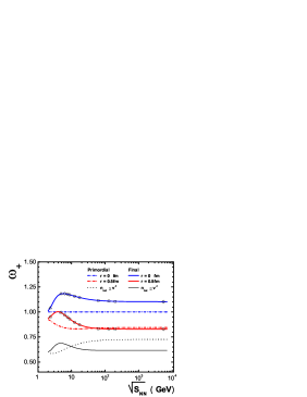
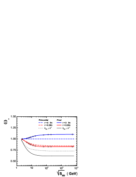
Figure 1: The scaled variances for positively (left) and negatively (right) charged particles along the chemical freeze-out line for central A+A collisions (see also Tables II and III). The calculations are done for the HG with Boltzmann statistics in the GCE. Symbols at the lines correspond to the specific collision energies pointed out in Table I. The dash-dotted lines correspond to the primordial and solid lines to final state values. The pair of upper lines show the ideal HG results, the pair of middle lines the VDW HG with hard-core radius $r=0.5$ fm. The lowest pair of lines corresponds to largest possible VDW suppression for the primordial (dotted) and final (solid) scaled variance, respectively. This largest VDW suppression happens at $n_{tot}\cong 1/v$.

$\sqrt{s_{NN}}$	$\;\omega_{+}$   Primordial				$\;\omega_{+}$   Final
[ GeV ]	$r=0$	$r=\!0.3$fm	$r=\!0.5$fm	$n_{tot}\cong v^{-1}$	$~{}r=0~{}$	$r=\!0.3$fm	$r=\!0.5$fm	$n_{tot}\cong v^{-1}$
$2.32$	1	0.977	0.915	0.587	1.040	1.017	0.952	0.613
$4.86$	1	0.951	0.853	0.612	1.181	1.118	0.995	0.688
$6.27$	1	0.943	0.843	0.629	1.183	1.106	0.970	0.681
$7.62$	1	0.939	0.837	0.642	1.178	1.091	0.948	0.671
$8.77$	1	0.936	0.835	0.651	1.173	1.079	0.932	0.663
$12.3$	1	0.931	0.832	0.669	1.158	1.051	0.898	0.645
$17.3$	1	0.928	0.832	0.684	1.145	1.029	0.873	0.632
$62.4$	1	0.928	0.840	0.715	1.115	0.989	0.835	0.617
$130$	1	0.929	0.843	0.722	1.109	0.983	0.830	0.617
$200$	1	0.929	0.844	0.723	1.107	0.981	0.830	0.617
$5500$	1	0.930	0.845	0.727	1.103	0.978	0.828	0.617

Table 2: The scaled variances of the primordial and final positively charged hadrons in central A+A collisions are presented at different c.m. energies $\sqrt{s_{NN}}$ (see also Fig. 1, left). The calculations are done for the HG with Boltzmann statistics in the GCE. The excluded volume parameter, $v=16\pi r^{3}/3$, is taken to be the same for all hadron species ($r=0$ corresponds to the ideal HG results). The condition $n_{tot}\cong 1/v$ corresponds to largest possible VDW total particle density, and this gives an upper limit of the VDW suppression effect for the scaled variances.

$\sqrt{s_{NN}}$	$\;\omega_{-}$   Primordial				$\;\omega_{-}$   Final
[ GeV ]	$r=0$	$r=\!0.3$fm	$r=\!0.5$fm	$n_{tot}\cong v^{-1}$	$~{}r=0~{}$	$r=\!0.3$fm	$r=\!0.5$fm	$n_{tot}\cong v^{-1}$
$2.32$	1	0.997	0.989	0.946	1.001	0.998	0.988	0.941
$4.86$	1	0.976	0.930	0.815	1.016	0.984	0.920	0.763
$6.27$	1	0.968	0.912	0.793	1.026	0.980	0.898	0.723
$7.62$	1	0.963	0.901	0.782	1.035	0.977	0.883	0.700
$8.77$	1	0.957	0.894	0.775	1.041	0.976	0.873	0.686
$12.3$	1	0.951	0.880	0.763	1.056	0.973	0.855	0.660
$17.3$	1	0.944	0.870	0.755	1.068	0.972	0.843	0.644
$62.4$	1	0.933	0.852	0.737	1.092	0.973	0.827	0.621
$130$	1	0.931	0.849	0.732	1.097	0.975	0.827	0.619
$200$	1	0.931	0.848	0.731	1.099	0.976	0.827	0.618
$5500$	1	0.930	0.846	0.727	1.103	0.978	0.828	0.617

Table 3: The same as in Table II, but for negatively charged hadrons (see also Fig. 2, right).

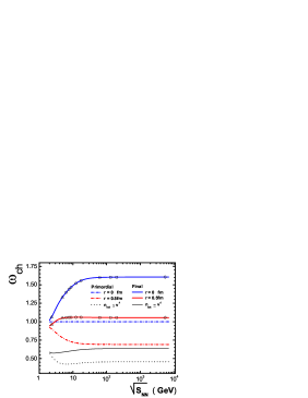
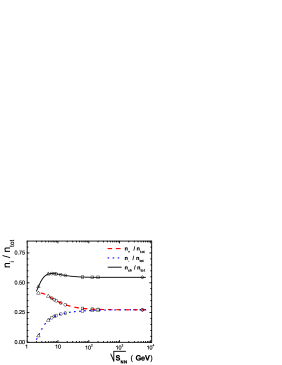
Figure 2: Left. The same as in Fig. 1, but for $\omega_{ch}$ (see also Table IV). Right. The ratios $n_{i}/n_{tot}=n_{i}^{id}/n_{tot}^{id}$ (see also Table I) for $i=+$ (dashed line), $i=-$ (dotted line), and $i=ch$ (solid line).

$\sqrt{s_{NN}}$	$\;\omega_{ch}$   Primordial				$\;\omega_{ch}$   Final
[ GeV ]	$r=0$	$r=\!0.3$fm	$r=\!0.5$fm	$n_{tot}\cong v^{-1}$	$~{}r=0~{}$	$r=\!0.3$fm	$r=\!0.5$fm	$n_{tot}\cong v^{-1}$
$2.32$	1	0.974	0.904	0.533	1.061	1.034	0.960	0.574
$4.86$	1	0.927	0.783	0.427	1.331	1.236	1.049	0.585
$6.27$	1	0.912	0.755	0.423	1.397	1.274	1.056	0.592
$7.62$	1	0.901	0.738	0.424	1.440	1.296	1.058	0.598
$8.77$	1	0.895	0.728	0.426	1.468	1.309	1.059	0.602
$12.3$	1	0.882	0.712	0.432	1.521	1.331	1.059	0.612
$17.3$	1	0.873	0.702	0.439	1.557	1.344	1.059	0.619
$62.4$	1	0.861	0.692	0.452	1.601	1.355	1.056	0.632
$130$	1	0.860	0.691	0.454	1.604	1.356	1.056	0.634
$200$	1	0.860	0.691	0.454	1.605	1.356	1.056	0.634
$5500$	1	0.860	0.691	0.454	1.605	1.356	1.056	0.634

Table 4: The same as in Table II, but for all charged hadrons (see also Fig. 2, left).

The excluded volume corrections, i.e. the factors $\exp\left(-vp/T\right)$ and $\left(1+v\sum_{i}x_{i}\right)^{-1}$, are calculated using the THERMUS package Thermus . Numerical optimization functions allow to solve the transcendental equation (21) for the pressure and, thus, find the hadron yields and fluctuations of the VDW HG. The thermodynamical parameters $T,~{}\mu_{B}$, and $\gamma_{S}$, the VDW suppression factor $R=\exp(-vp/T)[1+v\sum_{i}x_{i}]$, and the particle number ratios $n_{i}/n_{tot}=n_{i}^{id}/n_{tot}^{id}$ (see also Fig. 2, right) along the chemical freeze-out line are presented in Table I. Once a suitable set of thermodynamical parameters is determined for each collision energy, the scaled variance of negatively, positively, and all charged particles can be calculated using Eq. (IV.1) for $\omega_{+}$ and similar equations for $\omega_{-}$, $\omega_{ch}$, with the correlators taken from Eq. (46). The resulting scaled variances are presented in Tables II-IV and Figs. 1 and 2 (left) as a function of $\sqrt{s_{NN}}$. The values of $\sqrt{s_{NN}}$ quoted in Tables I-IV and marked in Figs. 1-2 correspond to the beam energies at SIS (2$A$ GeV), AGS (11.6$A$ GeV), SPS ($20A$, $30A$, $40A$, $80A$, and $158A$ GeV), colliding energies at RHIC ($\sqrt{s_{NN}}=62.4$ GeV, $130$ GeV, and $200$ GeV), and LHC ($\sqrt{s_{NN}}=5500$ GeV). Both the primordial and final state scaled variances are presented. To make a correspondence with real measurements, both strong and electromagnetic decays should be taken into account, while weak decays should be omitted.

Some features of the results should be mentioned. The values $\omega_{\pm}=\omega_{ch}=1$ are shown by the dashed-dotted lines in Figs. 1-2. They correspond to the primordial fluctuations in the ideal HG ($r=0$). The bump in $\omega_{+}$ for final state particles seen in Fig. 1 at the small collision energies is due to a correlated production of proton and $\pi^{+}$ meson from $\Delta^{++}$ decays. This single resonance contribution dominates in $\omega_{+}$ at small collision energies (small temperatures), but becomes relatively unimportant at the high collision energies.

The number of negative particles is relatively small, $\langle N_{-}\rangle\ll\langle N_{+}\rangle$, at low collision energies (see Fig. 2, right). For the hard-core radius $r=0.5$ fm, this region corresponds ’small’ particle number density, $vn_{tot}\ll 1$. It then follows, for the primordial values, $\omega_{\pm}\cong 1-2vn_{\pm}$ and $\omega_{ch}\cong 1-2vn_{ch}$. Thus, the VDW suppression effects are seen at low collision energy for positively charged and all charged particles (Fig. 1 and 2), and are absent for negatively charged particles (Fig. 1, right).

At high collision energies (large $T$) one finds $n_{-}\cong n_{+}$ as seen from Fig. 2, right. For the hard-core radius $r=0.5$ fm, Fig. 1 shows the asymptotic values of 0.85 for the primordial and 0.83 for the final scaled variances $\omega_{\pm}$ in the VDW HG, instead of 1 and 1.1, respectively, in the ideal HG. Thus, one observes about 15% and 25% VDW excluded volume suppression for, respectively, the primordial and final values of $\omega_{\pm}$. The upper limit of the VDW suppression effects for the scaled variances is obtained at $n_{tot}\cong 1/v$ and is presented in Figs. 1-2. The approximate relations both at small density, $\omega_{j}\cong 1-2vn_{j}$, and high density, $\omega_{j}\cong 1-n_{j}/n_{tot}$, demonstrate that VDW suppression of $j$th fluctuations is proportional to $j$th density in the HG. This explains why the VDW suppression for the primordial $\omega_{ch}$ seen in Fig. 2 is approximately the same as for $\omega_{+}$ at small collision energy and 2 times larger than that for $\omega_{\pm}$ at high collision energies.

A comparison of the primordial scaled variances with those for final hadrons demonstrates that the fluctuations increase in GCE ideal HG for each hadron species (see Eq. (16)) for positive, as well as for negative, and all charged hadrons (see Figs. 1-2). In the VDW HG the behavior is more complicated. At high collision energies, as demonstrated in Fig. 1, they even decrease for $\omega_{\pm}$ after resonance decays. This unexpected behavior follows from Eqs. (44) and (46). Calculating (46) one finds that only one term, $\sum_{R}\langle N_{R}\rangle\langle n_{i}n_{j}\rangle$, coming from resonance decays gives a positive contribution to the $\langle\Delta N_{j}\Delta N_{k}\rangle$ correlator. Other terms in the right hand side of Eq. (46) appear due to particle-resonance and resonance-resonance (anti)correlations in the VDW HG. As seen from Eq. (44) these terms are negative and, thus, suppress the scaled variances for the final state particles. The resulting effect from resonance decays is defined by the competition of two effects: decays into more than one $j$th particle against particle-resonance and resonance-resonance anticorrelations. Multi-particle decays lead to increase the fluctuations, while the anticorrelations because of the excluded volume lead to decrease them. For all charged particles the multi-particle decays win and $\omega_{ch}$ always increases due to resonance decays as seen from Fig. 2. This same is true for $\omega_{+}$ at small collision energies. The opposite situation takes place for $\omega_{\pm}$ at high collision energies. Anticorrelations because of the excluded volume overcome the multi-particle decay contributions, and $\omega_{\pm}$ decreases as seen from Fig. 1.

VI summary

The hadron multiplicity fluctuations in relativistic nucleus-nucleus collisions have been considered in the statistical hadron-resonance gas model. We study the effect of the van der Waals excluded volume on the hadron distribution scaled variances. In the present paper we restrict ourself to the grand canonical calculations within the Boltzmann statistics approximation.

If the proper volume parameter is the same for different hadron species, the particle number ratios remain unchanged and equal to those in the ideal hadron-resonance gas. Therefore, with rescaling of the total volume $V$ one may compensate the excluded volume suppression of the hadron densities leaving the hadron yields the same as in the ideal hadron-resonance gas. In the present paper it has been demonstrated that the multiplicity fluctuations are suppressed in the van der Waals gas. This suppression is qualitatively different from that of the particle yields. In contrast to the average multiplicities, the suppression of multiplicity fluctuations can not be removed by rescaling of the total volume of the system.

In this work we have considered two ‘reasonable‘ values of hard-sphere radii, $r=0.3fm$ and $r=0.5fm$, as well as the limiting behavior of the VDW suppression. Estimates of possible excluded volume suppression effects of particle number fluctuations from existing data in A+A collisions will be the subject of future studies.

- (1) J. Cleymans, H. Oeschler, K. Redlich, and S. Wheaton, Phys. Rev. C 73, 034905 (2006).
- (2) F. Becattini, J. Manninen, and M. Gaździcki, Phys. Rev. C 73, 044905 (2006).
- (3) A. Andronic, P. Braun-Munzinger, J. Stachel, Nucl. Phys. A 772, 167 (2006).
- (4) S.V. Afanasev et al., [NA49 Collaboration], Phys. Rev. Lett. 86, 1965 (2001); M.M. Aggarwal et al., [WA98 Collaboration], Phys. Rev. C 65, 054912 (2002); J. Adams et al., [STAR Collaboration], Phys. Rev. C 69, 044905 (2003); C. Roland et al., [NA49 Collaboration], J. Phys. G 30 S1381 (2004); Z.W. Chai et al., [PHOBOS Collaboration], J. Phys. Conf. Ser. 37, 128 (2005); M. Rybczynski et al. [NA49 Collaboration], J. Phys. Conf. Ser. 5, 74 (2005).
- (5) H. Appelshauser et al. [NA49 Collaboration], Phys. Lett. B 459, 679 (1999); D. Adamova et al., [CERES Collaboration], Nucl. Phys. A 727, 97 (2003); T. Anticic et al., [NA49 Collaboration], Phys. Rev. C 70, 034902 (2004); S.S. Adler et al., [PHENIX Collaboration], Phys. Rev. Lett. 93, 092301 (2004); J. Adams et al., [STAR Collaboration], Phys. Rev. C 71, 064906 (2005).
- (6) H. Heiselberg, Phys. Rep. 351, 161 (2001); S. Jeon and V. Koch, Review for Quark-Gluon Plasma 3, eds. R.C. Hwa and X.-N. Wang, World Scientific, Singapore, 430-490 (2004) [arXiv:hep-ph/0304012].
- (7) M. Gazdzicki, M. I. Gorenstein, and S. Mrowczynski, Phys. Lett. B 585, 115 (2004); M. I. Gorenstein, M. Gazdzicki and O. S. Zozulya, Phys. Lett. B 585, 237 (2004).
- (8) I.N. Mishustin, Phys. Rev. Lett. 82, 4779 (1999); Nucl. Phys. A 681, 56c (2001); H. Heiselberg and A.D. Jackson, Phys. Rev. C 63, 064904 (2001).
- (9) M.A. Stephanov, K. Rajagopal, and E.V. Shuryak, Phys. Rev. Lett. 81, 4816 (1998); Phys. Rev. D 60, 114028 (1999); M.A. Stephanov, Acta Phys. Polon. B 35, 2939 (2004).
- (10) V.V. Begun, M. Gaździcki, M.I. Gorenstein, and O.S. Zozulya, Phys. Rev. C 70, 034901 (2004); V.V. Begun, M.I. Gorenstein, and O.S. Zozulya, Phys. Rev. C 72, 014902 (2005); A. Keränen, F. Becattini, V.V. Begun, M.I. Gorenstein, and O.S. Zozulya, J. Phys. G 31, S1095 (2005); F. Becattini, A. Keränen, L. Ferroni, and T. Gabbriellini, Phys. Rev. C 72, 064904 (2005); V.V. Begun, M.I. Gorenstein, A.P. Kostyuk, and O.S. Zozulya, Phys. Rev. C 71, 054904 (2005); J. Cleymans, K. Redlich, and L. Turko, Phys. Rev. C 71, 047902 (2005); J. Phys. G 31, 1421 (2005); V.V. Begun, M.I. Gorenstein, A.P. Kostyuk, and O.S. Zozulya, J. Phys. G 32, 935 (2006). V.V. Begun and M.I. Gorenstein, Phys. Rev. C 73, 054904 (2006).
- (11) V.V. Begun, M.I. Gorenstein, M. Hauer, V.P. Konchakovski, and O.S. Zozulya, Phys.Rev. C 74 044903 (2006).
- (12) V.V. Begun, M. Gaździcki, M.I. Gorenstein, M. Hauer, V.P. Konchakovski, and B. Lungwitz arXiv:nucl-th/0611075.
- (13) V.P. Konchakovski, S. Haussler, M.I. Gorenstein, E.L. Bratkovskaya, M. Bleicher, and H. Stöcker, Phys. Rev. C 73, 034902 (2006); V.P. Konchakovski, M.I. Gorenstein, E.L. Bratkovskaya, and H. Stöcker, Phys. Rev C 74, 064911 (2006).
- (14) M. Gaździcki and M.I. Gorenstein, Phys. Lett. B 640, 155 (2006).
- (15) B. Lungwitzt et al. [NA49 Collaboration], arXiv:nucl-ex/0610046.
- (16) S. Jeon and V. Koch, Phys. Rev. Lett. 83, 5435 (1999).
- (17) D.H. Rischke, M.I. Gorenstein, H. Stöcker, and W. Greiner, Z. Phys. C 51, 485 (1991); J. Cleymans, M.I. Gorenstein, J. Stalnacke, and E. Suhonen, Z. Phys. C 8, 347 (1993).
- (18) Granddon D. Yen, M.I. Gorenstein, W. Greiner, and Shin Nan Yang, Phys. Rev. C 56, 2210 (1997); M.I. Gorenstein, H. Stöcker, Granddon D. Yen, Shin Nan Yang, and W. Greiner, J. Phys. G 24, 1777 (1998); Granddon D. Yen and M.I. Gorenstein, Phys. Rev. C 59, 2788 (1999),
- (19) M.I. Gorenstein, V.K. Petrov, and G.M. Zinovjev, Phys. Lett. B 106, 327 (1981); M.I. Gorenstein, W. Greiner, and Shin Nan Yang, J.Phys. G 24, 725 (1998); M.I. Gorenstein, M. Gaździcki, and W. Greiner, Phys. Rev. C 72, 024909 (2005).
- (20) J. Cleymans and K. Redlich, Phys. Rev. Lett. 81, 5284 (1998).
- (21) S. Wheaton and J. Cleymans, arXiv:hep-ph/0407174.