Elliptic flow in transport theory and hydrodynamics

Abstract

We present a new direct simulation Monte-Carlo method for solving the relativistic Boltzmann equation. We solve numerically the 2-dimensional Boltzmann equation using this new algorithm. We find that elliptic flow from this transport calculation smoothly converges towards the value from ideal hydrodynamics as the number of collisions per particle increases, as expected on general theoretical grounds, but in contrast with previous transport calculations.

Ultrarelativistic nucleus-nucleus collisions at the Relativistic Heavy Ion Collider (RHIC) have been argued to create a “perfect liquid”, with an extremely low viscosity Tannenbaum:2006ch . The essential piece of evidence is the large magnitude of elliptic flow at RHIC Ackermann:2000tr , which is as large as predicted by ideal-fluid models (which assume zero viscosity). Elliptic flow is an azimuthal asymmetry in the momentum distribution of particles, projected onto the plane transverse to the beam direction ($z$ axis): in a collision between two nuclei with non-zero impact parameter, more particles are emitted parallel to impact parameter ($x$ axis) than perpendicular to it ($y$ axis). This asymmetry results from the almond shape of the overlap region between the colliding nuclei, which is transformed into a momentum asymmetry by pressure gradients Ollitrault:1992bk : microscopically, elliptic flow results from the interactions between the produced particles, and is therefore a key observable of the dense matter produced at RHIC.

In the microscopic language of particle physics, ideal fluid and low viscosity translate into small mean free path of a particle between two collisions or, equivalently, large rescattering cross sections between the “partons” created in a collision. The description of the system in terms of partons is itself questionable at the early, dense stage of the collision, but it is nevertheless a helpful, intuitive picture. The natural question which arises then is: how large must the partonic cross section be in order to achieve ideal-fluid behavior, i.e., local thermal equilibirum? How many partonic collisions are needed?

In this paper, we address this issue by solving numerically a relativistic Boltzmann equation, and comparing the results with relativistic hydrodynamics. It is well known that the Boltzmann equation reduces to hydrodynamics when the mean free path is small (see Marle for a rigorous proof in the relativistic case). Numerically, however, it has been found Molnar:2004yh that hydrodynamics produces larger elliptic flow (by 30-40%) than the Boltzmann equation. In this paper, we address this issue using a different method. A possible explanation for the discrepancy found in Molnar:2004yh is suggested at the end of this paper.

The primary limitation of the Boltzmann equation is that it only applies to a dilute system, where the mean free path of a particle is much larger than the distance between particles, so that one need only consider two-body collisions, many-body collisions occurring at a much lower rate. There is no reason to believe that the RHIC liquid is dilute: interactions are nonperturbative, so that both the mean free path and the distance between particles are of order $1/T$, where $T$ is the temperature. Clearly, the Boltzmann equation cannot be used to directly simulate a heavy-ion collision; nevertheless, it has the potential of giving us a grasp on deviations to thermalization.

The relativistic formula for the collision rate between two beams of particle densities $n_{1}$ and $n_{2}$, and arbitrary velocities ${\bf v_{1}}$ and ${\bf v_{2}}$ can be written as Landau :

$$\frac{dN_{\rm coll}}{dtd^{3}{\bf x}}=\sigma n_{1}n_{2}\sqrt{|{\bf v_{1}}-{\bf v_{2}}|^{2}-|{\bf v_{1}}\times{\bf v_{2}}|^{2}/c^{2}},$$ (1)

where $\sigma$ is the scattering cross section. There are several methods for implementing this collision rate in Monte-Carlo algorithms. The most widely used method Zhang:1999bd ; Molnar:2001ux is the ZPC algorithm Zhang:1997ej : this algorithm treats particles as hard spheres, which collide when their distance in the center-of-mass frame is smaller than $r\equiv\sqrt{\sigma/\pi}$. An alternative method is the stochastic collision algorithm proposed by Xu and Greiner Xu:2004mz .

Here, we implement a new algorithm, where relativistic effects are incorporated in a physically transparent way. The second term under the square root in Eq. (1) is the relativistic correction. It is simply understood, in the case of colliding hard spheres, as a geometrical effect resulting from the Lorentz contraction of the spheres. We take this contraction into account, in the Monte-Carlo simulation, by replacing spheres with oblate spheroids, whose polar axis is the direction of motion. As with the other algorithms, Lorentz covariance and locality are broken in the sense that collisions occur instantaneously at a finite distance. However, these violations are small if the system is dilute Molnar:2001ux , which is required by the Boltzmann equation. The difference with the ZPC algorithm is that the collision time is determined directly in the laboratory frame, not in the center-of-mass frame.

For sake of simplicity, we consider a two-dimensional gas of massless particles in the transverse plane $(x,y)$. We thus neglect an important feature of the dynamics of heavy-ion collisions, the fast longitudinal expansion. As will be shown below, this is not crucial for elliptic flow, which is essentially unaffected by the longitudinal expansion. Initial conditions for the $N$ particles are generated randomly according to a gaussian distribution in coordinate space, and an isotropic, thermal distribution in momentum space:

$$\frac{dN}{d^{2}{\bf x}d^{2}{\bf p}}=\frac{N}{4\pi^{2}R_{x}R_{y}T^{2}}\exp\left(-\frac{x^{2}}{2R_{x}^{2}}-\frac{y^{2}}{2R_{y}^{2}}-\frac{p_{t}}{T(x,y)}\right),$$ (2)

with $R_{y}>R_{x}$ and $p_{t}\equiv\sqrt{p_{x}^{2}+p_{y}^{2}}$. The temperature $T(x,y)$ is determined as a function of the local particle density per unit area, $n_{2d}$ according to $n_{2d}\propto T^{2}$, the equation of state of a massless ideal gas in 2 dimensions.

Particles interact via $2\to 2$ elastic collisions. We assume for simplicity that the total elastic cross section $\sigma_{2d}$ is independent of the center-of-mass energy $s$. (In 2 dimensions, the cross section has the dimension of a length.) This is implemented in a Monte-Carlo calculation by treating each particle as a rod (due to Lorentz contraction) of length $r={1\over 2}\sigma_{2d}$ perpendicular to the velocity. Equivalently, for each pair of colliding particles, one can assume that particle 1 has length $2r$ and particle 2 is pointlike (see Fig. 1). The impact parameter of the collision is

$$d=-\frac{{\bf e_{z}}\cdot(({\bf x_{2}}-{\bf x_{1}})\times({\bf v_{2}}-{\bf v_{1}})/c)}{1-{\bf v_{1}}\cdot{\bf v_{2}}/c^{2}}$$ (3)

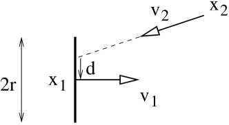
Figure 1: Picture of a collision between a particle 1 of size $\sigma_{2d}=2r$ and a pointlike particle $2$. The impact parameter $d$, as defined in Eq. (3), is negative.

This quantity is Lorentz invariant. Our collision algorithm is deterministic: the scattering angle in the center-of-mass frame $\theta^{*}$ is determined as a function of $d$, as in classical mechanics. The results presented here are obtained with an isotropic differential cross section, i.e., $\theta^{*}=\pi(1-d/r)$. This prescription ensures that particles move away from each other after the collision and do not collide again.

We now define two dimensionless numbers relevant to this problem. The average particle density per unit surface $n_{2d}$ is 

$$n_{2d}=\frac{N}{4\pi R_{x}R_{y}}.$$ (4)

The typical distance between two particles is $n_{2d}^{-1/2}$, while The mean free path of a particle between two collisions is $\lambda=1/(\sigma_{2d}n_{2d})$. The ratio of these two lengths is the dilution parameter $D$:

$$D\equiv\frac{n_{2d}^{-1/2}}{\lambda}=\sigma_{2d}n_{2d}^{1/2}.$$ (5)

As explained above, applicability of Boltzmann theory requires $D\ll 1$. In addition, locality and covariance require that the interaction length be much smaller than the mean free path Molnar:2001ux ; Zhang:1997ej . In two dimensions, the interaction length is $\sigma_{2d}$, and $\sigma_{2d}/\lambda=D^{2}$: locality and covariance are thus recovered in the limit $D\ll 1$.

The second dimensionless number is the Knudsen number ${\rm Kn}$, which characterizes the degree of equilibration by comparing $\lambda$ with the system size $R$. The latter quantity can be measured by any average of $R_{x}$ and $R_{y}$. A natural choice for elliptic flow is Bhalerao:2005mm

$$R\equiv\left(\frac{1}{R_{x}^{2}}+\frac{1}{R_{y}^{2}}\right)^{-1/2}.$$ (6)

The Knudsen number is then defined as

$${\rm Kn}\equiv\frac{\lambda}{R}=\frac{1}{\sigma_{2d}n_{2d}R}.$$ (7)

Hydrodynamics is the limit ${\rm Kn}\ll 1$, while the limit ${\rm Kn}\gg 1$ corresponds to free-streaming particles. The values of $D$ and ${\rm Kn}$ can be tuned by varying the cross section $\sigma_{2d}$ and the number of particles $N$.

Note that the mean free path is a local quantity, which depends on space-time coordinates: in particular, it increases as the system expands. Strictly speaking, $D$ and ${\rm Kn}$ defined by Eqs. (5) and (7) are initial values. Dimensional analysis suggests that they are the relevant control parameters for this problem.

Solving the Boltzmann equation in the hydrodynamic limit requires both $D\ll 1$ and ${\rm Kn}\ll 1$. This in turn requires a huge number of particles $N$ in the Monte-Carlo simulation: inverting the above equations, one obtains (assuming $R_{x}\simeq R_{y}$ for simplicity)

$$N\simeq\frac{8\pi}{D^{2}{\rm Kn}^{2}}.$$ (8)

Since the computing time scales grows with $N$ like $N^{3/2}$, one cannot implement arbitrarily small values of $D$ and ${\rm Kn}$. Instead, we choose to study numerically the dependence of elliptic flow on $D$ and ${\rm Kn}$, and extrapolate to the hydro limit $D={\rm Kn}=0$.

Figure 2: Variation of the elliptic flow $v_{2}$ with the Knudsen number, ${\rm Kn}$, for several values of the dilution parameter $D$. The statistical error on each point is $\delta v_{2}=7\times 10^{-4}$. For each value of $D$, Monte-Carlo results are fitted using Eq. (9).

Fig. 2 presents our results for the average elliptic flow $v_{2}\equiv\langle\cos 2\phi\rangle=\langle(p_{x}^{2}-p_{y}^{2})/(p_{x}^{2}+p_{y}^{2})\rangle$. The aspect ratio of the initial distribution is $R_{y}=1.5R_{x}$, and the Monte-Carlo simulation has been pushed to very large times ($t=100R$), so that all collisions are taken into account. Quite naturally, $v_{2}$ decreases monotonically to 0 as ${\rm Kn}$ increases towards the free-streaming limit ${\rm Kn}\to+\infty$. For a given value of $D$, the variation with ${\rm Kn}$ is very well described by the simple formula proposed in Bhalerao:2005mm :

$$v_{2}=\frac{v_{2}^{h}}{1+{\rm Kn}/{\rm Kn}_{0}},$$ (9)

where the parameters $v_{2}^{h}$ and ${\rm Kn}_{0}$ are fit to our Monte-Carlo results. $v_{2}^{h}$ is the limiting value of $v_{2}$ when ${\rm Kn}\to 0$, expected to coincide with $v_{2}$ from hydrodynamics in the limit $D\to 0$. Surprisingly, the value of $v_{2}^{h}$ depends very little on $D$: $v_{2}^{h}=0.102\pm 0.003$. This means that the hydrodynamic limit is more general than the Boltzmann equation and applies even if the system is not dilute. Unlike $v_{2}^{h}$, the parameter ${\rm Kn}_{0}$ strongly depends on $D$. We do not have a simple explanation for this dependence. However, only the limit $D\ll 1$ has a well-defined physical interpretation, as it corresponds to the Boltzmann equation. For larger values of $D$, locality and causality are broken, and the physical interpretation of the results is less clear. For $D\ll 1$, our fit gives ${\rm Kn}_{0}=0.70\pm 0.03$.

An independent hydro calculation with the same initial conditions was done using the same code as in Ref. Ollitrault:1992bk . For sake of consistency Molnar:2004yh , the equation of state of the fluid is that of a two-dimensional ideal gas (i.e., the equation of state of a dilute gas, as modeled by the Boltzmann equation), whose velocity of sound is $c_{s}=c/\sqrt{2}$ Heinz:2002rs . The average $v_{2}$ at $t=100R$ is $v_{2}^{\rm hydro}=0.101\pm 0.003$ (the error bar in the hydro calculation is due to the fact that the calculation is pushed to very large times). This is compatible with the value $v_{2}^{h}$ obtained from the Boltzmann calculation: Boltzmann transport theory and ideal hydrodynamics agree in the limit ${\rm Kn}\to 0$, as expected.

The Knudsen number is closely related to the average number of collisions per particle $\bar{n}_{\rm coll}$. From the definition, Eq. (7), one expects that the number of collisions per particle is $\sim 1/{\rm Kn}$. The proportionality constant can be computed exactly for a gaussian distribution in the limit ${\rm Kn}\gg 1$ Heiselberg:1998es , which yields the relation

$$\bar{n}_{\rm coll}\equiv\frac{2N_{\rm coll}}{N}=\frac{4\sqrt{2}}{\pi^{3/2}\sqrt{1+\epsilon}}K\!\left(\frac{2\epsilon}{1+\epsilon}\right){\rm Kn}^{-1}\simeq\frac{1.6}{\rm Kn},$$ (10)

where the factor 2 means that each collision involves 2 particles, $\epsilon=(R_{y}^{2}-R_{x}^{2})/(R_{y}^{2}+R_{x}^{2})$ is the initial eccentricity, and $K(x)$ is the complete elliptic integral of the first kind. We used this formula to check numerically that our algorithm produces the right number of collisions for large ${\rm Kn}$. In addition, our numerical results show that the product $\bar{n}_{\rm coll}{\rm Kn}$ is remarkably constant for all values of ${\rm Kn}$, so that Eq. (10) holds within a few percent. Using Eq. (9), this shows that an average of $2.3$ (resp. $9.1$) collisions per particle are required to achieve 50% (resp. 80%) of the hydrodynamic “limit” on $v_{2}$.

Figure 3: Time dependence of the average elliptic flow $v_{2}$ from the transport model, from the corresponding 2-dimensional hydro calculation, and from usual 3-dimensional hydro with Bjorken longitudinal expansion.

Fig. 3 compares the time-dependence of elliptic flow in hydro and in the transport model. The subtle point is that the convergence of $v_{2}(t)$ towards hydro as ${\rm Kn}\to 0$ is not uniform: for a given value of ${\rm Kn}$, deviations from hydro are large at early times, and tend to decrease afterwards. More precisely, it can be shown, following the same methods as in Ref. Heiselberg:1998es , that the early-time behavior is $v_{2}\propto t^{3}$ in the transport model, and $v_{2}\propto t^{2}$ in hydro. This is compensated by the late-time behavior: $v_{2}$ decreases slowly at large times in hydro (not seen in the figure), while $v_{2}$ from the transport model stays constant after the last collision has occurred.

Can our 2-dimensional results be used in the context of heavy-ion collisions? The essential difference in 3 dimensions is the fast longitudinal expansion due to the strong Lorentz contraction of the colliding nuclei. Elliptic flow, however, is a purely transverse observable which is little affected by the longitudinal expansion: Fig. 3 displays a comparison between the average elliptic flow computed in 2-dimensional hydro and in 3-dimensional hydro with Bjorken longitudinal expansion (the initial time in this calculation is $\tau_{0}=R/4$, corresponding to $\tau_{0}\simeq 0.4$ fm/c in a semicentral Au-Au collision) Bjorken:1982qr . Both yield similar results for the magnitude and the time-dependence of $v_{2}$.

One can reasonably expect that deviations from hydro are similar in 2 dimensions and in 3 dimensions. The number of collisions per particle, $\bar{n}_{\rm coll}$, is not the right quantity for carrying out the comparison (neither the transport opacity Molnar:2001ux ): in 3 dimensions, $\bar{n}_{\rm coll}$ is large at early times (with a fixed partonic cross section, $\bar{n}_{\rm coll}$ diverges like $\ln\tau_{0}^{-1}$ as the initial time $\tau_{0}$ goes to 0), but these collisions do not produce much elliptic flow (see Fig. 3). As argued in Ref. Bhalerao:2005mm , the Knudsen number should be evaluated at the time when elliptic flow develops $t\sim R/c_{s}$, with $c_{s}\simeq 1/\sqrt{3}$ in the quark-gluon plasma phase. The mean free path is $\lambda=1/\sigma n$ with $n=(1/ct)(1/S)(dN/dy)$ and $S=4\pi R_{x}R_{y}$, hence

$$\frac{1}{\rm Kn}=\sigma\frac{1}{S}\frac{dN}{dy}\frac{c_{s}}{c}.$$ (11)

$dN/dy$ is the total (charged+neutral) multiplicity. For a semi-central Au-Au collision at RHIC, $(1/S)(dN/dy)\simeq 0.8$ mb^-1. With this definition of ${\rm Kn}$, we expect that Eq. (9) should hold approximately in 3 dimensions, with ${\rm Kn}_{0}\sim 0.7$. Table 1 gathers numerical estimates obtained using the same values of $\sigma$ as in Ref.Molnar:2004yh . For $\sigma=20$ mb, corresponding to a QCD cross-section of 47 mb, the transport result should be only $\simeq 10-15\%$ below hydro.

Table 1: Expected values of $v_{2}$ for semi-central Au-Au collisions at RHIC. For each value of the cross section, we quote the value of the equivalent Debye-screened, leading order QCD cross section Molnar:2004yh .

Isotropic $\sigma$ [mb]	Debye-screened $\sigma$ [mb]	${\rm Kn}$	$v_{2}/{v_{2}^{\rm hydro}}$
3	7	0.72	0.49
8	19	0.27	0.72
20	47	0.11	0.87

For this value of the cross section, Molnar and Huovinen find that $v_{2}$ from the transport calculation is lower by 30% than $v_{2}$ from hydro Molnar:2004yh . Furthermore, the dependence of their results on $\sigma$ is at variance with our results. Using Eqs. (9) and (11), the deviations from ideal hydro should decrease as $1/\sigma$ as $\sigma$ increases. This is very general: dissipative effects are expected to be linear in the viscosity $\eta$, which scales like $1/\sigma$. The discrepancy with hydro should be at least twice smaller with $\sigma=47$ mb than with $\sigma=20$ mb, which is clearly not the case in Fig. 1 of Ref. Molnar:2004yh . In our opinion, this cannot be attributed to dissipative effects.

The origin of the problem may be the dilution condition $D\ll 1$, which is not satisfied in previous transport calculations. The trick to reduce $D$ in the ZPC cascade algorithm is the “parton subdivision technique”: one multiplies the number of particles $N$ by a large number $l$, and one divides the partonic cross section $\sigma$ by $l$, so that the Knudsen number ${\rm Kn}$ is unchanged. The distance between particles in three dimensions is $n^{-1/3}$, which replaces $n_{2d}^{-1/2}$ in Eq. (5). Taking parton subdivision into account, one obtains $D=\sigma n^{2/3}l^{-1/3}$. The average particle density in a semicentral Au-Au collision at time $t=R/c_{s}$ is $2.5$ fm^-3 Bhalerao:2005mm . With $\sigma=20$ mb and $l=180$ Molnar:2004yh , $D\simeq 0.65$, which is not very small compared to unity. The situation is worse at early times due to the longitudinal expansion: $D\simeq 1.1$ at $\tau_{0}=0.6$ fm/c. For ${\rm Kn}=0.11$, carrying out the calculation with $D\simeq 1$ leads to overestimate the deviation from hydro by at least a factor of 2 (see Fig. 2). The reason why previous calculations were done with such large values of $D$ is that small values are hard to achieve numerically: in 3 dimensions, Eq. (8) is replaced with $N\propto D^{-3}{\rm Kn}^{-3}$, and the computing time grows like $N^{4/3}\propto D^{-4}{\rm Kn}^{-4}$. This was our motivation for studying first the 2-dimensional case.

In summary, we have implemented a new algorithm for solving the relativistic Boltzmann equation. We have studied the convergence of the relativistic Boltzmann equation to relativistic hydrodynamics. Since this requires both a dilute system ($D\ll 1$) and a small mean free path (${\rm Kn}\ll 1$), which is costly in terms of computer time, we have restricted our study to two dimensions. This preliminary study has only addressed the average value of the elliptic flow; differential results as a function of $p_{t}$, as well as results on $v_{4}$, will be presented in a forthcoming publication. We have shown that the average elliptic flow computed in the transport algorithm converges smoothly towards the hydrodynamics value as the strength of final-state interactions increases. Isotropic partonic cross sections of 3 mb and 20 mb should produce respectively $\sim 50\%$ and $\sim 90\%$ of the hydro value for $v_{2}$.

References

- (1) M. J. Tannenbaum, Rept. Prog. Phys. 69, 2005 (2006).
- (2) K. H. Ackermann et al., Phys. Rev. Lett. 86, 402 (2001).
- (3) J. Y. Ollitrault, Phys. Rev. D 46, 229 (1992).
- (4) C. Marle, Annales Poincare Phys.Theor. 10,67 (1969).
- (5) D. Molnar and P. Huovinen, Phys. Rev. Lett. 94, 012302 (2005).
- (6) L. D. Landau, E. M. Lifshitz, The Classical Theory of Fields, 4th Edition (Pergamon Press, 1975), page 36.
- (7) B. Zhang, C. M. Ko, B. A. Li and Z. w. Lin, Phys. Rev. C 61, 067901 (2000); Z. W. Lin, C. M. Ko, B. A. Li, B. Zhang and S. Pal, Phys. Rev. C 72, 064901 (2005).
- (8) D. Molnar and M. Gyulassy, Phys. Rev. C 62, 054907 (2000); Nucl. Phys. A 697, 495 (2002) [Erratum-ibid. A 703, 893 (2002)].
- (9) B. Zhang, Comput. Phys. Commun. 109, 193 (1998). B. Zhang, M. Gyulassy and Y. Pang, Phys. Rev. C 58, 1175 (1998).
- (10) Z. Xu and C. Greiner, Phys. Rev. C 71, 064901 (2005).
- (11) R. S. Bhalerao, J. P. Blaizot, N. Borghini and J. Y. Ollitrault, Phys. Lett. B 627, 49 (2005).
- (12) S. A. Voloshin and A. M. Poskanzer, Phys. Lett. B 474, 27 (2000).
- (13) U. W. Heinz and S. M. H. Wong, Phys. Rev. C 66, 014907 (2002).
- (14) H. Heiselberg and A. M. Levy, Phys. Rev. C 59, 2716 (1999).
- (15) J. D. Bjorken, Phys. Rev. D 27, 140 (1983).