Universality of Decay out of Superdeformed Bands in the 190 Mass Region

Abstract

Superdeformed nuclei in the 190 mass region exhibit a striking universality in their decay-out profiles. We show that this universality can be explained in the two-level model of superdeformed decay as related to the strong separation of energy scales: a higher scale related to the nuclear interactions, and a lower scale caused by electromagnetic decay. Decay-out can only occur when separate conditions in both energy regimes are satisfied, strongly limiting the collective degrees of freedom available to the decaying nucleus. Furthermore, we present the results of the two-level model for all decays for which sufficient data are known, including statistical extraction of the matrix element for tunneling through the potential barrier.

I Introduction

It is well known that, for a major–to–minor axis ratio of about 2, a new set of shell closures and magic numbers occurs in many nuclei. Such superdeformed (SD) states are one of the most striking predictions of the shell model aberg90 . High electric quadrupole moments and small centrifugal stretching mark these states as fundamentally different from their normally deformed (ND) isomers twin90 . This contrast has stimulated an abundance of experimental and theoretical studies, yet several pressing questions persist aberg90 ; twin90 ; nolan88 . Of these, perhaps the most interesting is the mechanism by which SD bands decay.

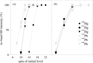
Figure 1: (a) Decay profiles of several SD bands near $A\approx 190$. Note how suddenly each decay-out occurs. (b) The profiles of (a), but shifted in angular momentum so that the leftmost points, the last point in which the SD band is experimentally observed to retain any strength, are aligned. In addition to the abruptness of their decay, the profiles are seen to exhibit a universal behavior. Both graphs are from Ref. wilson05a .

After their formation at high angular momentum, typically via heavy ion collisions, these nuclei decay to the yrast SD rotational band, and then uniformly down that band by $E2$ transitions. The SD bands are observed

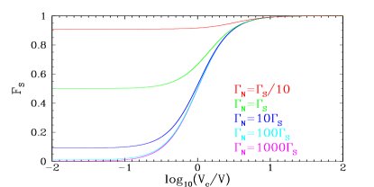
Figure 2: (Color online) SD branching ratio $F_{S}$, calculated in the two-level model and showing the onset of universality. Universality of the decay profiles arises from the fact that interband decay is nearly forbidden until conditions are favorable in both energy regimes, at which point SD strength vanishes quickly. The sudden transition from intraband to interband decay occurs when both $\Gamma_{N}\gtrsim\Gamma_{S}$ and $V\gtrsim V_{c}$, where the critical tunneling matrix element $V_{c}$ is given by Eq. (29). When both conditions are satisfied, the curves are thus nearly identical, giving rise to the observed universality of decay profiles.

to retain their strength through many states, even after they are no longer yrast, with negligible losses. Then, quite suddenly, the SD band loses almost all of its strength over just one or two states [see Fig. 1(a)], although the nucleus is still well above the SD bandhead. After a series of statistical decays through unrelated states, the nuclei continue via $E1$-dominated decays in an ND rotational band twin90 ; nolan88 .

By far the most SD decays have been observed in the “classic” 190 mass region. Recently, Wilson and collaborators wilson05a demonstrated a striking feature of SD decay in this region: the decay profiles, when corrected for differing angular momenta, are nearly identical [Fig. 1(b)]. This universality of decays is to be contrasted with mere abruptness, a feature which has been acknowledged for some time. Indeed, it was noted as early as Ref. shimizu93 that a purely statistical model would be insufficient to explain true universality, i.e. strong consistency between different decay profiles. Likewise, a chaos-assisted phenomenon cannot, of itself, generate universality.

The purpose of this article is to demonstrate that within the two-level model of SD decay-out, the decay profile is universal. In this model, the branching ratio is completely determined by four parameters: the detuning $\Delta\equiv\varepsilon_{N}-\varepsilon_{S}$, a tunneling matrix element $V$, and electromagnetically induced broadenings for the SD and ND wells, $\Gamma_{S}$ and $\Gamma_{N}$, respectively. Because nuclear forces are very much stronger than electromagnetic, there is a strong separation of scales $V,\Delta\gg\Gamma_{S},\Gamma_{N}$. We show that the decay-out only occurs when conditions have become favorable in both energy regimes. As a consequence, decay occurs not only very suddenly, but also in a limited region of the model’s full parameter space. Within this subspace, branching ratios are highly insensitive to changes in the parameters, resulting in the universality observed in experiment.

Figure 2 illustrates these findings. It depicts the calculated value of the in-band branching ratio $F_{S}$ for various ratios $\Gamma_{S}/\Gamma_{N}$. $V_{c}$, a simple function of $\Delta$ and $\Gamma_{S}/\Gamma_{N}$ in the two-level model, sets the scale $V$ must achieve to allow decay. Universality is evident from the figure: if either $\Gamma_{S}/\Gamma_{N}$ or $V_{c}/V$ is too large, no decay can occur. On the other hand, as both cross critical values, $F_{S}$ suddenly vanishes. Furthermore, the curves converge in this, the decay-allowed limit, resulting in a universal profile in good agreement with the experimental results of Fig. 1. However, the connection between this theoretical universality and the experimentally observed universality still needs to be made, because the abscissas of the two plots (Figs. 1 and 2) are not the same. This connection will require a theoretical understanding of the angular momentum dependence of $V$, which in turn requires a more detailed understanding of the barrier between the two wells.

The outline of the paper is as follows. We first briefly review the two-level model in Section II. Section III presents the model’s results, on which Fig. 2 is based. Section III further includes a numerical analysis of all SD decays for which sufficient data are known. Section IV gives our conclusions.

II Two-level model of SD decay

Theoretical efforts to describe the SD decay process have centered on a potential function of both nuclear quadrupole deformation and angular momentum. Vigezzi and collaborators noted early on that a double well in the deformation more accurately models the experimental data than any alternative vigezzi90a . In this picture, the shape of the tunnel barrier and the two wells varies as the nucleus sheds angular momentum, and the states of the ND and SD wells are broadened by their respective couplings to the electromagnetic field. Shortly thereafter, Khoo et al. khoo93a conclusively demonstrated that these electromagnetic widths must be much less than the inter-level spacings in each well. The most appropriate picture for SD decay is thus found to be two sets of discrete, slightly broadened states, connected by matrix elements to tunnel through the barrier.

The two-level model for SD decay SB is given by keeping only one level in each well, the decaying SD level and the ND level with nearest energy (see Fig. 3). Since the role of additional ND levels is principally to steal decay strength from the first CSBPRL ; dzyublik03a , it is now well established that going beyond this level of approximation is not useful for most heavy-nuclei SD decays.

Figure 3: Schematic diagram of the two-level model of SD decay. In each well of the double-well potential, only one level is kept. $\varepsilon_{N}$ and $\varepsilon_{S}$ are the unperturbed energies of the isolated ND and SD states, which are connected by a tunneling matrix element $V$. The two states have electromagnetic decay rates $\Gamma_{N}/\hbar$ and $\Gamma_{S}/\hbar$, respectively.

II.1 Green’s Function Description of SD Decay

The Hamiltonian of the two-level model is a sum of three terms: $H=H_{W}+H_{T}+H_{D}$. In the basis of the two isolated levels, the first term is diagonal:

$$H_{W}=\left(\begin{array}[]{cc}\varepsilon_{S}&0\\ 0&\varepsilon_{N}\end{array}\right),$$ (1)

where $\varepsilon_{i}$ is the energy of state $i$. $H_{W}$ generates time evolution within each well: its related retarded Green’s function is $G_{W}(E)=\left(E-H_{W}+i0^{+}\right)^{-1}$.

The second term,

$$H_{T}=\left(\begin{array}[]{cc}0&V\\ V&0\end{array}\right),$$ (2)

allows tunneling through the barrier. Here we have chosen the relative phases of the basis states $|S\rangle$ and $|N\rangle$ such that $V$ is positive, without loss of generality. Together, $H_{W}$ and $H_{T}$ form a simple problem common to many introductory quantum mechanics texts.

The remaining term, $H_{D}=H_{EM}+H_{c}$, gives the electromagnetic decay of the two levels. $H_{EM}$ is composed of the electromagnetic (harmonic oscillator) modes of the environment, and $H_{c}$ gives their couplings to the nucleus. In this case, it is not necessary to treat the particulars of these terms; rather we work at the level of the experimentally determined decay rates $\Gamma_{S}/\hbar$ and $\Gamma_{N}/\hbar$ phenomnote . The self-energy due to $H_{D}$ is

$$\Sigma=-\frac{i}{2}\left(\begin{array}[]{cc}\Gamma_{S}&0\\ 0&\Gamma_{N}\end{array}\right).$$ (3)

Dyson’s Equation

$$G(E)=\left(\left[G_{W}(E)\right]^{-1}-H_{T}-\Sigma\right)^{-1}$$ (4)

gives the Green’s function of the full system, summing the effects of $\Sigma$ and $H_{T}$ to all orders. Treating the physics of the two wells ($G_{W}$), electromagnetic decay ($\Sigma$), and the barrier ($H_{T}$) on the same footing in this way is essential to a complete description of SD decay-out: all three play equally important roles in determining experimental observables, such as branching ratios. The full Green’s function of the two-level model is thus

$$G \equiv \left(\begin{array}[]{cc}G_{SS}&G_{SN}\\ G_{NS}&G_{NN}\end{array}\right)$$ (10)

$$= \left[(E-\varepsilon_{S}+i\Gamma_{S}/2)(E-\varepsilon_{N}+i\Gamma_{N}/2)-V^{2}\right]^{-1}$$

$$\times\left(\begin{array}[]{cc}E-\varepsilon_{N}+i\Gamma_{N}/2&V\\ V&E-\varepsilon_{S}+i\Gamma_{S}/2\end{array}\right).$$

At $t=0$, the nucleus is localized in the SD well by virtue of its previous, measurable $E2$ decay. For later times, then, the probability to find the nucleus in the SD or ND well is given by $P_{i}(t)=|\tilde{G}_{iS}(t)|^{2}$, where $i=S,N$ respectively. Here

$$\tilde{G}_{iS}(t)=\int^{\infty}_{-\infty}\frac{dE}{2\pi}G_{iS}(E)\mathrm{e}^{-iEt/\hbar},$$ (11)

the Fourier transform of $G_{ij}(E)$, is the retarded propagator from $S$ to $i$.

The resulting probabilities are

$$P_{N}(t)=\frac{2V^{2}}{|\hbar\omega|^{2}}\mathrm{e}^{-\overline{\Gamma}t/\hbar}\left[\cosh\left(\omega_{i}t\right)-\cos\left(\omega_{r}t\right)\right]$$ (12)

and

$$\begin{split}P_{S}(t)=\frac{V^{2}}{|\hbar\omega|^{2}}\mathrm{e}^{-\overline{\Gamma}t/\hbar}\left(\frac{\hbar\omega_{i}+\Gamma^{\prime}}{\Gamma^{\prime}-\hbar\omega_{i}}\mathrm{e}^{\omega_{i}t}+\frac{\Gamma^{\prime}-\hbar\omega_{i}}{\hbar\omega_{i}+\Gamma^{\prime}}\mathrm{e}^{-\omega_{i}t}+\right.\\ \left.+\frac{i\hbar\omega_{r}+\Gamma^{\prime}}{i\hbar\omega_{r}-\Gamma^{\prime}}\mathrm{e}^{i\omega_{r}t}+\frac{i\hbar\omega_{r}-\Gamma^{\prime}}{i\hbar\omega_{r}+\Gamma^{\prime}}\mathrm{e}^{-i\omega_{r}t}\right).\end{split}$$ (13)

Here, $\overline{\Gamma}\equiv(\Gamma_{N}+\Gamma_{S})/2$ and $\Gamma^{\prime}\equiv(\Gamma_{N}-\Gamma_{S})/2$, while the real and imaginary parts of the complex Rabi frequency $\omega$ are given by

$$\omega_{r,i}^{2}=\frac{\sqrt{\Omega^{2}+4\Delta^{2}\Gamma^{\prime 2}}\pm\Omega}{2\hbar^{2}},\quad\Omega\equiv 4V^{2}+\Delta^{2}-\Gamma^{\prime 2},$$ (14)

respectively, where the “$+$” sign is used for the real part, and the “$-$” for the imaginary. As Eqs. (12) and (13) demonstrate, $\omega_{i}$ is associated with decoherence due to coupling with the electromagnetic field, while $\omega_{r}$ is analogous to the real Rabi frequency of a closed two-well system.

The branching ratios $F_{i}=\left(\Gamma_{i}/\hbar\right)\int_{0}^{\infty}dtP_{i}(t)$ are found by time-integrating the probabilities. The results are SB

$$F_{N}=\frac{\Gamma_{N}\Gamma^{\downarrow}/\left(\Gamma_{N}+\Gamma^{\downarrow}\right)}{\Gamma_{S}+\Gamma_{N}\Gamma^{\downarrow}/\left(\Gamma_{N}+\Gamma^{\downarrow}\right)}$$ (15a)

$$F_{S}=\frac{\Gamma_{S}}{\Gamma_{S}+\Gamma_{N}\Gamma^{\downarrow}/\left(\Gamma_{N}+\Gamma^{\downarrow}\right)},$$ (15b)

where

$$\Gamma^{\downarrow}\equiv\frac{2\overline{\Gamma}V^{2}}{\Delta^{2}+\overline{\Gamma}^{2}}.$$ (16)

Equations (15) are the expected results for series decay out of a two-level problem. In this light, it is clear that $\Gamma^{\downarrow}$ is simply the net rate for the nucleus, starting in the SD well, to tunnel irreversibly through the barrier.

These results allow us to extract information about the potential barrier from experiment. In particular, the values determined by a typical SD decay experiment are $F_{S}=1-F_{N}$ and $\Gamma_{S}$, while $\Gamma_{N}$ can be estimated by applying the cranking model to a Fermi gas density of states dossing95a . From Eq. (15), we find

$$\Gamma^{\downarrow}=\Gamma_{S}\bigg{/}\left(\frac{F_{S}}{F_{N}}-\frac{\Gamma_{S}}{\Gamma_{N}}\right).$$ (17)

II.2 Determination of $V$

To uniquely extract $V$ itself requires $\Delta$, which in turn implies detailed knowledge of the spectrum in the ND well. In the absence of this, we consider the entire statistical ensemble of two-level models, each characterized by a different value of the unknown variable $\Delta$.

To proceed, we construct a probability density function $\mathcal{P}(\Delta)$, which gives the statistical weight each value of $\Delta$ has in the ensemble. The simplest ansatz for the distribution of energy levels in the ND well is the “structureless” Wigner surmise mehta :

$$P(s)=\frac{\pi}{2}se^{-\pi s^{2}/4},$$ (18)

where $s$ is the level spacing in units of its average value $D_{N}$. $\Delta$ is the detuning between the SD state and its nearest ND neighbor; thus its magnitude must be less than half the spacing $sD_{N}$ between the ND levels just above and just below the SD level. Given this spacing, therefore, $\Delta$ is drawn from the rectangular probability density

$$\mathcal{P}_{s}(\Delta)=\frac{1}{sD_{N}}\Theta\left(\frac{s}{2}-\frac{|\Delta|}{D_{N}}\right),$$ (19)

where $\Theta$ is the Heaviside step function. The total probability theorem yields the desired result CSBPRL :

$$\mathcal{P}(\Delta)=\int_{0}^{\infty}\mathcal{P}_{s}(\Delta)P(s)ds=\frac{\pi}{2D_{N}}\mathrm{erfc}\left(\sqrt{\pi}\frac{|\Delta|}{D_{N}}\right),$$ (20)

where $\mathrm{erfc}(x)$ denotes the complementary error function of $x$.

A probabilistic statement like Eq. (20) obviates the need for exact knowledge of $\Delta$. To arrive at the probability density function $\mathcal{P}(V)$, one need only perform an elementary change of variables:

$$\mathcal{P}(V)=2\mathcal{P}(\Delta)\left|\frac{d\Delta(V)}{dV}\right|,$$ (21)

where the factor 2 results from our choice of phase for $V$. Here, $\left|\Delta(V)\right|$ is a function, not the random variable $\Delta$; it is found from Eq. (16) to be

$$\left|\Delta(V)\right|=\sqrt{\frac{2\overline{\Gamma}}{\Gamma^{\downarrow}}\left(V^{2}-V_{min}^{2}\right)},$$ (22)

where $V_{min}=\sqrt{\frac{1}{2}\Gamma^{\downarrow}\overline{\Gamma}}$ is the smallest $V$ consistent with the two-level model. $\mathcal{P}(V)$ is thus seen to be CSBPRL ; deltanote

$$\mathcal{P}(V)=\left\{\begin{array}[]{ll}\frac{2\pi}{D_{N}}\frac{\overline{\Gamma}V}{\Gamma^{\downarrow}|\Delta(V)|}\mathrm{erfc}\left(\sqrt{\pi}\frac{|\Delta(V)|}{D_{N}}\right),&V>V_{min}\\ 0&\textrm{otherwise}\end{array}\right..$$ (23)

A probability distribution such as Eq. (23) represents the most one can say about $V$ without microscopic knowledge of the ND well. The mean of $\mathcal{P}(V)$ is

$$\langle V\rangle=\sqrt{\frac{\Gamma^{\downarrow}}{2\overline{\Gamma}}}\left[\frac{D_{N}}{4}+\mathcal{O}\left(\frac{\overline{\Gamma}^{2}}{D_{N}}\right)\right],$$ (24)

while the standard deviation is

$$\sigma_{V}=\sqrt{\frac{\Gamma^{\downarrow}}{2\overline{\Gamma}}}\left[D_{N}\sqrt{\frac{1}{3\pi}-\frac{1}{16}}+\mathcal{O}\left(\overline{\Gamma}\right)\right].$$ (25)

$\sigma_{V}/\langle V\rangle\approx 84\%$, indicating that $\mathcal{P}(V)$ is well peaked about $\langle V\rangle$, and thus this mean provides a good measure of the likely value of $V$.

The Wigner surmise (18), provides a reasonable, neutral guess at the spacings of states in the ND well. It is closely related, and may be considered a good approximation, to the level distribution of the Gaussian orthogonal ensemble mehta . Nevertheless, it is straightforward to reproduce the preceeding analysis, substituting a level-spacing density of choice for Eq. (18).

III Results for the 150 and 190 Mass Regions

Table 1 gives the values of $\Gamma^{\downarrow}$ and $\langle V\rangle$ for all SD decays for which the four parameters, $F_{N}$; $\Gamma_{S}$; $\Gamma_{N}$; and $D_{N}$, are known. In the table, we have further defined the series rate to irreversibly leave the SD band:

$$\Gamma_{out}/\hbar=\frac{\Gamma_{N}\Gamma^{\downarrow}}{\Gamma_{N}+\Gamma^{\downarrow}}/\hbar=\Gamma_{S}\frac{F_{N}}{F_{S}}/\hbar.$$ (26)

It is $\Gamma_{out}$, directly extractable from experimental results, which competes with $\Gamma_{S}$ to determine whether a nucleus will decay out of or remain within the SD band.

Table 1: Results of the two-level model, for all SD decays for which sufficient data (branching ratios, $\Gamma_{S}$, $\Gamma_{N}$, and $D_{N}$) are known. $I$ is the nuclear spin quantum number. Note that $\langle V_{c}\rangle$ and $\Gamma_{S}/\left(\Gamma_{S}+\Gamma_{N}\right)$ do not depend on $F_{S}$. The rightmost column gives the sources of the experimental inputs and the estimates of $\Gamma_{N}$ and $D_{N}$.

nucleus($I$)	$F_{S}$		$\Gamma_{S}$		$\Gamma_{N}$		$D_{N}$		$\Gamma^{\downarrow}$		$\Gamma_{out}$		$\langle V\rangle$		$\langle V_{c}\rangle$		$\frac{\Gamma_{S}}{\Gamma_{S}+\Gamma_{N}}$		Refs.
			(meV)		(meV)		(eV)		(meV)		(meV)		(eV)		(eV)
192Hg(12)	0.	74	0.	128	0.	613	135.		0.	049	0.	045	8.	7	14.	0	0.	173	lauritsen00a ; wilson05a
192Hg(10)	0.	08	0.	050	0.	733	89.		2.	7	0.	58	41.		5.	6	0.	064	lauritsen00a ; wilson05a
192Pb(16)	$>$0.	99	0.	487	0.	192	1,362.		$<$0.	0050	$<$0.	0049	$<$29.		288.		0.	717	wilson03a ; wilson04a
192Pb(14)	0.	98	0.	266	0.	201	1,258.		0.	0056	0.	0054	34.		237.		0.	570	wilson03a ; wilson04a
192Pb(12)	0.	66	0.	132	0.	200	1,272.		0.	10	0.	067	170.		201.		0.	398	wilson03a ; wilson04a
192Pb(10)	0.	12	0.	048	0.	188	1,410.		1.	9$\dagger$	0.	35	1000.	$\dagger$	160.		0.	203	wilson03a ; wilson04a
192Pb(8)	$<$0.	25	0.	016	0.	169	1,681.		$>$0.	067	$>$0.	048	$>$250.		120.		0.	086	wilson03a ; wilson04a
194Hg(12)	0.	58	0.	097	4.	8	16.	3	0.	071	0.	070	0.	49	0.	58	0.	020	khoo96a ; kuehn97a ; moore97a ; kruecken01a
194Hg(10)	$<$0.	09	0.	039	4.	1	26.	2	$>$0.	44	$>$0.	40	$>$2.	1	0.	64	0.	0094	khoo96a ; kuehn97a ; moore97a ; kruecken01a
194Hg(12)	0.	60	0.	108	21.		344.		0.	072	0.	072	5.	0	6.	1	0.	0051	lauritsen02a
194Hg(10)	0.	03	0.	046	20.		493.		1.	6	1.	5	35.		5.	9	0.	0023	lauritsen02a
194Hg(12)	0.	60	0.	086	1.	345	19.		0.	060	0.	057	0.	97	1.	2	0.	060	moore97a ; wilson05a
194Hg(10)	$\leq$0.	05	0.	033	1.	487	14.		$\geq$1.	1	$\geq$0.	63	$\geq$3.	0	0.	52	0.	022	moore97a ; wilson05a
194Hg(15)	0.	90	0.	230	4.	0	26.	5	0.	026	0.	026	0.	52	1.	5	0.	054	moore97a ; kruecken01a
194Hg(13)	0.	84	0.	110	4.	5	19.	9	0.	021	0.	021	0.	34	0.	77	0.	024	moore97a ; kruecken01a
194Hg(11)	$<$0.	07	0.	048	6.	4	7.	2	$>$0.	71	$>$0.	64	$>$0.	60	0.	15	0.	0074	moore97a ; kruecken01a
194Pb(10)	0.	90	0.	045	0.	08	21,700.		0.	0053	0.	0050	1100.		3300.		0.	36	willsau93a ; lopezmartens96a ; hauschild97a ; kruecken01a
194Pb(8)	0.	62	0.	014	0.	50	2,200.		0.	0087	0.	0086	72.		90.		0.	027	willsau93a ; lopezmartens96a ; hauschild97a ; kruecken01a
194Pb(6)	$<$0.	09	0.	003	0.	65	1,400.		$>$0.	032	$>$0.	030	$>$77.		20.		0.	005	willsau93a ; lopezmartens96a ; hauschild97a ; kruecken01a
194Pb(12)	$>$0.	99	0.	125	0.	476	236.		$<$0.	0013	$<$0.	0013	$<$2.	7	26.	9	0.	208	kruecken01a ; wilson04a
194Pb(10)	0.	90	0.	045	0.	470	244.		0.	0051	0.	0050	6.	1	18.		0.	087	kruecken01a ; wilson04a
194Pb(8)	0.	65	0.	014	0.	445	273.		0.	0077	0.	0076	8.	8	12.		0.	031	kruecken01a ; wilson04a
194Pb(6)	$<$0.	04	0.	003	0.	405	333.		$>$0.	088	$>$0.	072	$>$39.		7.		0.	007	kruecken01a ; wilson04a
152Dy(28)	0.	60	10.	0	17.		220.		11.		6.	7	35.		33.		0.	37	lauritsen02a
152Dy(26)	0.	19	7.	0	17.		194.		140.	$\dagger$	30.		120.	$\dagger$	26.		0.	29	lauritsen02a

$\dagger$Calculated statistically, as explained in the appendix.

The dynamics of SD decay is a consequence of the strong separation of energy scales,

$$\Gamma_{S},\Gamma_{N}\ll D_{N},\langle V\rangle,$$ (27)

exhibited in Table 1. In the 190 mass region, particularly, we find that parameters relating to the potential double-well, such as $D_{N}$ and $V$, are 10’s to 1000’s of electron–Volts, while those relating to electromagnetic decay are fractions of meV. This is to be expected, since nuclear forces are, of course, many orders of magnitude stronger than electromagnetic ones.

Each of these energy scales has a typical rate associated with it: oscillations within the two-level system are characterized by $\omega_{r}$, whereas $\overline{\Gamma}/\hbar$ gives the typical rate for electromagnetic decay in Eqs. (12)–(13). Since $\hbar\omega_{r}\gg\overline{\Gamma}$, it is clear that SD decay is primarily a coherent process: a nucleus generally undergoes thousands of virtual Rabi oscillations during a single decay event. Only if both $V$ and $\Delta$ were of order meV or smaller could the decay be incoherent, and such “accidental” near-degeneracies are masked by the fact that, since $\Gamma^{\downarrow}\approx 0$, when $V$ is very small, the nucleus cannot leave the SD band. Moreover, the probability for $\Delta$ to be of order $\overline{\Gamma}$ is seen from Eq. (20) to be $\sim\overline{\Gamma}/D_{N}$.

Equation (15b) can be rewritten:

$$F_{S}=1-\frac{1}{1+\left(V_{c}/V\right)^{2}+\Gamma_{S}/\Gamma_{N}},$$ (28)

where

$$V_{c}^{2}\equiv\left(\Delta^{2}+\overline{\Gamma}^{2}\right)\frac{\Gamma_{S}/\Gamma_{N}}{1+\Gamma_{S}/\Gamma_{N}}.$$ (29)

The critical tunneling matrix element $V_{c}$ can be extracted from experiment via a statistical approach similar to that described for $V$ in Section II.2, except that the result does not depend on $\Gamma^{\downarrow}$ or $F_{S}$. The resulting average values $\langle V_{c}\rangle$ are tabulated in Table 1.

According to Eq. (28), only two dimensionless parameters, $\Gamma_{S}/\Gamma_{N}$ and $V_{c}/V$, play a role in determining the branching ratios; each corresponds to one of the problem’s two energy scales. It is clear from Table 1 that the first, $\Gamma_{S}/\Gamma_{N}$, decreases dramatically over the course of each SD band’s decay-out. This can be understood physically as a relaxation of the nucleus’s centrifugal stretching, and consequent reduced coupling to the electric quadrupole field, as its spin lowers.

We extracted $\langle V\rangle$ using the experimental branching ratios; thus it would be circular to make use of those values in our discussion of $F_{S}$’s universality. Instead we note that Eqs. (15b) and (28) have the limit

$$\lim_{V\rightarrow\infty}F_{S}=\frac{\Gamma_{S}}{\Gamma_{S}+\Gamma_{N}},$$ (30)

and that, in the two-level model, $F_{S}$ is a monotonically decreasing function of $V$. Values of this limit are given in Table 1. As we move down each decay chain, it is clear that the experimental branching ratios converge to these values, and hence we conclude that $V_{c}/V$, too, is decreasing quickly during each decay chain. This also is to be expected: $V$ depends exponentially on the barrier height kruecken96a , which decreases as the ND well drops further below the SD one in energy.

Figure 2 shows $F_{S}$ as a function of $V_{c}/V$ and $\Gamma_{S}/\Gamma_{N}$. As both $\Gamma_{S}/\Gamma_{N}$ and $V_{c}/V$ decrease, the SD branching ratio decreases to an abrupt plateau. Furthermore, within the decay-allowed region

$$\Gamma_{N}\gtrsim\Gamma_{S}\,\cap\,V\gtrsim V_{c}$$ (31)

all the curves quickly become nearly identical.

Thus, we explain the universal nature of the decay-out profiles as follows: SD decay-out is only allowed when suitably low values of both $\Gamma_{S}/\Gamma_{N}$ and $V_{c}/V$ are achieved, both of which decrease quickly with decreasing spin. The nucleus, therefore, enters the region of allowed decay-out very suddenly, moving down the curves from a case of very high in-band intensity to one of almost complete decay-out; high in-band intensity corresponds to the long chains of pre-decay SD states observed in experiment, while the rapid transition into the decay-allowed region forms the abrupt decay profiles. However, once the system enters the decay-allowed region, the branching ratios saturate, and hence are no longer sensitive to further changes in the parameters, as Fig. 2 shows. The decay profile is consequently universal.

If ${}^{152}\mathrm{Dy}$ is a representative example, the variation of $\Gamma_{S}/\Gamma_{N}$ in the 150 mass region is somewhat slower than in the 190 region, although $V_{c}/V$ still changes dramatically, as seen from $F_{S}$’s approach to its $V\rightarrow\infty$ limit. Since rapid entry into the decay-allowed region is a necessary precondition of universal behavior, we expect that, as more data become available for these nuclei, a somewhat lesser degree of universality will be observed.

IV Conclusions

The two-level model has elsewhere CSBPRL ; dzyublik03a been shown to be the simplest description of the SD decay-out process which still encapsulates the essential physics. It describes a two-step decay: first, the nucleus undergoes mainly coherent Rabi oscillations between the SD and ND wells, after which it finally decays into one band or the other. By using a statistical approach, the two-level model can extract as much information as is possible from decay experiments, including the Hamiltonian matrix element for tunneling through the potential barrier, which is of direct relevance to nuclear structure. Table 1 demonstrates the results of this technique for all decays with sufficient data, to date.

Moreover, the most striking property of SD decay-out in the 190 mass region, universality of the decay profiles, is seen to correspond to universal behavior of the branching ratio in the two-level model. The two-level branching ratio is completely determined by two dimensionless parameters, $\Gamma_{S}/\Gamma_{N}$ and $V_{c}/V$, each of which corresponds to one of the two disparate energy scales of the problem. Decay-out only occurs when both of these parameters are decreasing rapidly. Thus, in the sector of parameter space for which decays are allowed, the branching ratios saturate and are insensitive to variations of the parameters. Assuming that the relationship between nuclear spin and barrier shape is reasonably consistent from nucleus to nucleus, the resulting decay profiles are necessarily similar.

Appendix

Equation (17) places a limit on the experimentally-determined quantities. Positivity of $\Gamma^{\downarrow}$ requires that

$$\Gamma_{N}>\Gamma_{out}$$ (32)

In only two decays of Table 1, ${}^{192}\mathrm{Pb}(10)$ and ${}^{152}\mathrm{Dy}(26)$, is this condition violated. While it is possible that this is due to a breakdown of the two-level approximation in these cases, in the absence of a physical argument for the near degeneracy of two or more ND levels, it is more likely that one or more of the input parameters is poorly known. $\Gamma_{N}$, in particular, is difficult to estimate, with uncertainty $\sigma_{\Gamma_{N}}\sim\Gamma_{N}$.

Thus, we estimate $\Gamma^{\downarrow}$ statistically for these two decays, assuming the true $\Gamma_{N}$ differs from the estimated value $\Gamma_{N}^{0}$ by a “cut” normal distribution:

$$\mathcal{P}(\Gamma_{N})=\left\{\begin{array}[]{ll}\frac{\mathcal{A}}{\Gamma_{N}^{0}\sqrt{2\pi}}\mathrm{e}^{-\left(\frac{\Gamma_{N}-\Gamma_{N}^{0}}{\sqrt{2}\Gamma_{N}^{0}}\right)^{2}},&\Gamma_{N}>\Gamma_{out}\\ 0&\textrm{otherwise}\end{array}\right.,$$ (33)

where the constant of renormalization due to the constraint is

$$\mathcal{A}=2\left\{\mathrm{erfc}\left[\frac{1}{\sqrt{2}}\left(\frac{\Gamma_{out}}{\Gamma_{N}^{0}}-1\right)\right]\right\}^{-1}.$$ (34)

Assuming that the two-level approximation is valid, the probability density function of $\Gamma^{\downarrow}$ follows:

$$\mathcal{P}(\Gamma^{\downarrow})=\mathcal{P}(\Gamma_{N})\left|\frac{d\Gamma_{N}}{d\Gamma^{\downarrow}}\right|=\left(\frac{\Gamma_{N}}{\Gamma^{\downarrow}}\right)^{2}\mathcal{P}(\Gamma_{N}),$$ (35)

where $\Gamma^{\downarrow}$ is the function of $\Gamma_{N}$ given by Eq. (17). For ${}^{192}\mathrm{Pb}(10)$ and ${}^{152}\mathrm{Dy}(26)$, Table 1 gives the median of this distribution as the typical value of $\Gamma^{\downarrow}$, from which $\langle V\rangle$ is found.

References

- (1) S. Åberg, Nucl. Phys. A 520 (1990) 35c.
- (2) P. J. Twin, Nucl. Phys. A 520 (1990) 17c.
- (3) P. J. Nolan and P. J. Twin, Annu. Rev. Nucl. Part. Sci. 38 (1988) 533; R. V. F. Janssens and T. L. Khoo, Annu. Rev. Nucl. Part. Sci. 41 (1991) 321; J. F. Sharpey-Schafer, Prog. Part. Nucl. Phys. 28 (1992) 187; T. L. Khoo, in Tunneling in Complex Systems, Proc. from the INT, Vol. 5, edited by S. Tomsovic (World Scientific, Singapore, 1998), p. 229.
- (4) A. N. Wilson, A. J. Sargeant, P. M. Davidson, and M. S. Hussein, Phys. Rev. C 71 (2005) 034319.
- (5) Y. R. Schimizu, E. Vigezzi, T. Døssing, and R. A. Broglia, Nucl. Phys. A 557 (1993) 99c.
- (6) E. Vigezzi, R. A. Broglia, and T. Døssing, Nucl. Phys. A 520 (1990a) 179c; E. Vigezzi, R. A. Broglia, and T. Døssing, Phys. Lett. B 249 (1990b) 163.
- (7) T. L. Khoo, T. Lauritsen, I. Ahmad, M. P. Carpenter, P. B. Fernandez, R. V. F. Janssens, E. F. Moore, F. L. H. Wolfs, Ph. Benet, P. J. Daly, et al., Nucl. Phys. A 557 (1993) 83c.
- (8) C. A. Stafford and B. R. Barrett, Phys. Rev. C 60 (1999) 051305(R).
- (9) D. M. Cardamone, C. A. Stafford, and B. R. Barrett, Phys. Rev. Lett. 91 (2003) 102502.
- (10) A. Ya. Dzyublik and V. V. Utyuzh, Phys. Rev. C 68 (2003) 024311.
- (11) The central role of electromagnetic processes in SD nuclei decay suggests such a phenomenological approach. A microscopic theory, while doubtless desirable in its own right, would also obscure much of the experimentally-relevant dynamics.
- (12) T. Døssing and E. Vigezzi, Nucl. Phys. A 587 (1995) 13.
- (13) M. L. Mehta, Random Matrices and the Statistical Theory of Energy Levels (Academic, New York, 1967).
- (14) Note that explicitly does not assume any particualr value of , as was claimed in Ref. wilson05a . Rather, it represents a weighted average over all values of .
- (15) T. Lauritsen, T. L. Khoo, I. Ahmad, M. P. Carpenter, R. V. F. Janssens, A. Korichi, A. Lopez-Martens, H. Amro, S. Berger, L. Calderin, et al., Phys. Rev. C 62 (2003) 044316.
- (16) A. N. Wilson, G. D. Dracoulis, A. P. Byrne, P. M. Davidson, G. J. Lane, R. M. Clark, P. Fallon, A. Görgen, A. O. Macchiavelli, and D. Ward, Phys. Rev. Lett. 90 (2003) 142501.
- (17) A. N. Wilson and P. M. Davidson, Phys. Rev. C 69 (2004) 041303(R).
- (18) T. L. Khoo, M. P. Carpenter, T. Lauritsen, D. Ackermann, I. Ahmad, D. J. Blumenthal, S. M. Fischer, R. V. F. Janssens, D. Nisius, E. F. Moore, et al., Phys. Rev. Lett. 76 (1996) 1583.
- (19) R. Kühn, A. Dewald, R. Krücken, C. Meier, R. Peusquens, H. Tiessler, O. Vogel, S. Kasemann, P. von Brentano, D. Bazzacco, et al., Phys. Rev. C 55 (1997) R1002.
- (20) E. F. Moore, T. Lauritsen, R. V. F. Janssens, T. L. Khoo, D. Ackermann, I. Ahmad, H. Amro, D. Blumenthal, M. P. Carpenter, S. M. Fischer, et al., Phys. Rev. C 55 (1997) R2150.
- (21) R. Krücken, A. Dewald, P. von Brentano, and H. A. Weidenmüller, Phys. Rev. C 64 (2001) 064316.
- (22) T. Lauritsen, M. P. Carpenter, T. Døssing, P. Fallon, B. Herskind, R. V. F. Janssens, D. G. Jenkins, T. L. Khoo, F. G. Kondev, A. Lopez-Martens, et al., Phys. Rev. Lett. 88 (2002) 042501.
- (23) P. Willsau, H. Hübel, W. Korten, F. Azaiez, M. A. Deleplanque, R. M. Diamond, A. O. Macchiavelli, F. S. Stephens, H. Kluge, F. Hannachi, et al., Z. Phys. A 344 (1993) 351.
- (24) A. Lopez-Martens, F. Hannachi, A. Korichi, C. Schück, E. Geuorguieva, Ch. Vieu, B. Haas, R. Lucas, A. Astier, G. Baldsiefen, et al., Phys. Lett. B 380 (1996) 18.
- (25) K. Hauschild, L. A. Bernstein, J. A. Becker, D. E. Archer, R. W. Bauer, D. P. McNabb, J. A. Cizewski, K.-Y. Ding, W. Younes, R. Krücken, et al., Phys. Rev. C 55 (1997) 2819.
- (26) R. Krücken, A. Dewald, P. von Brentano, D. Bazzacco, and C. Rossi-Alvarez, Phys. Rev. C 54 (1996) 1182.