Femtoscopic correlations in multiparticle production and beta-decay

Abstract

The basics of formalism of femtoscopic and spectroscopic correlations are given, the orthogonal character of these correlations is stressed. The similarity and difference of femtoscopic correlations in multiparticle production and beta-decay is discussed.

I INTRODUCTION

The momentum correlations of two or more particles at small relative momenta in their center-of-mass (c.m.) system are widely used to study space-time characteristics of the production processes on a level of fm $=10^{-15}$ m, so serving as a correlation femtoscopy tool. Particularly, for non-interacting identical particles, like photons or, to some extent, pions, these correlations result from the interference of the production amplitudes due to the symmetrization requirement of quantum statistics (QS) GGLP60 ; gkp71 ; KP72 ; kop74 ; pod89 .

The momentum QS correlations were first observed as an enhanced production of the pairs of identical pions with small opening angles (GGLP effect GGLP60 ). Later on, Kopylov and Podgoretsky settled the basics of correlation femtoscopy in more than 20 papers (see a review pod89 ) and developed it as a practical tool; particularly, they suggested to study the interference effect in terms of the correlation function, proposed the mixing techniques to construct the uncorrelated reference sample and clarified the role of the space–time characteristics of particle production in various physical situations.

There exists gkp71 ; KP72 ; kop74 ; pod89 ; shu73 ; coc74 ; KP75 an analogy of the momentum QS correlations of photons with the space–time correlations of the intensities of classical electromagnetic fields used in astronomy to measure the angular radii of stellar objects based on the superposition principle (HBT effect) hbt . This analogy is sometimes misunderstood and the momentum correlations are mixed up with the space-time (HBT) correlations in spite that their orthogonal character and thus the absence of the former in astronomy measurements due to extremely large space-time extent of stellar objects (and vice versa) was already pointed out in early paper KP75 (see also lyu98 ).

Note that though the space-time (HBT) correlations are absent in subatomic measurements, they can still be used in laboratory as an intensity-correlation spectroscopy tool allowing one to measure the spectral line shape and width (see glw66 ; pkd67 and references therein). In fact, the QS space-time correlations give the information about shape and width of the three-momentum distribution (including the angular one) of the quanta coming from a distant source and can be considered as a spectroscopy tool in this more general sense.

The momentum correlations of particles emitted at nuclear distances are also influenced by the effect of final state interaction (FSI) koo ; gkw79 ; ll1 ; BS86 ; bgj90 . Thus the effect of the Coulomb interaction dominates the correlations of charged particles at the relative momenta $2k^{*}$ in the two-particle rest frame smaller than the inverse Bohr radius $|a|^{-1}$ of the two-particle system, respectively suppressing or enhancing the production of particles with like or unlike charges.

Though the FSI effect complicates the correlation analysis, it is an important source of information allowing for the coalescence femtoscopy (see, e.g., sy81 ; lyu88 ; mro93 ; sh99 ), the correlation femtoscopy with unlike particles ll1 ; BS86 ; bgj90 including the access to the relative space–time asymmetries in particle production LLEN95 ; ali95 ; vol97 ; sof97 ; lpx ; led03 ; mis98 ; led02 ; blu02 ; ada03a ; kis04 ; led04 and a study of strong interactions between specific particles led02 ; kis04 ; led04 .

In fact, the femtoscopic Coulomb correlations were observed more than 70 years ago when a sensitivity of the differential beta-decay rate to the nucleus charge and radius has been established fer34 .

The paper is organized now as follows. In sections II-IV we give the basics of formalism of femtoscopic and spectroscopic correlations. The similarity and difference of femtoscopic correlations in multiparticle production and beta-decay is discussed in section V. We conclude in section VI. For recent results from femtoscopy of multiparticle production processes, one can inspect reviews led04 ; lis05 ; cso05 ; led06 .

II FEMTOSCOPIC QS CORRELATIONS

II.1 Formalism

The correlation function ${\mathcal{R}}(p_{1},p_{2})$ of two particles with four-momenta $p_{1}$ and $p_{2}$ is usually defined as the ratio of the measured momentum distribution of the two particles to the reference one obtained by mixing particles from different events of a given class, normalized to unity at sufficiently large relative momenta.

For identical pions or kaons, the effect of the strong FSI is usually small and the effect of the Coulomb FSI can be in first approximation simply corrected for (see slape and references therein). The corrected correlation function is then determined by the QS symmetrization only. The space-time information contained in the momentum QS correlations can be extracted based on the Kopylov-Podgoretsky (KP) formalism of independent one-particle classical emitters that are characterized by their production (excitation) four-coordinates, four-velocities, lifetimes and decay amplitudes. The KP formalism is valid on the following assumptions:

(i) The multiplicity of produced particles is assumed sufficiently large to neglect the influence of conservation laws.

(ii) An independent or incoherent particle emission is assumed, i.e. the coherent contribution of multiparticle emitters is neglected (this contribution can be eventually taken into account with the help of the suppression parameter $\lambda$).

(iii) The mean freeze-out phase space density is assumed sufficiently small so that the correlation function of two particles emitted with a small relative momentum $Q=2k^{*}$ in their c.m. system is mainly determined by their mutual correlation.

(iv) The momentum dependence of the one-particle emission probabilities is assumed inessential when varying the particle four-momenta $p_{1}$ and $p_{2}$ by the amount characteristic for the correlation effect. This so-called smoothness assumption requires the components of the mean space-time distance between particle emitters much larger than those of the space-time extent of the emitters.

The probability amplitude to observe a particle with the four-coordinate $x$ from an emitter A decaying at the four-coordinate $x_{\rm A}$ can depend on $x$ through the relative four-coordinate $x-x_{\rm A}$ only and so can be written in the form:

$$\langle x|\psi_{\rm A}\rangle=(2\pi)^{-4}\int d^{4}\kappa~{}u_{\rm A}(\kappa)\exp[i\kappa(x-x_{\rm A})].$$ (1)

We assume here that after the production the emitter moves along a classical trajectory and decays according to the exponential decay law. Such a classical treatment of the decay is often applied also to resonances (see, e.g., Led92 ; ll96 ; cp01 ). It is justified for a heavy emitter with the energy spectrum of the decay particle substantially wider than the emitter width. One can avoid the classical treatment of the emitter decay by considering $x_{\rm A}$ in Eq. (1) as the emitter production (excitation) four-coordinate and adding, in the case of a negligible emitter space-time extent, the theta-function $\theta(t-t_{\rm A})$.

The probability amplitude to observe the particle with the four-momentum $p$ is

$$\langle p|\psi_{\rm A}\rangle=\int d^{4}x~{}\langle p|x\rangle\langle x|\psi_{\rm A}\rangle=u_{\rm A}(p)\exp(-ipx_{\rm A}),$$ (2)

where $\langle p|x\rangle=\exp(-ipx)$. The probability amplitude to observe identical spin-0 bosons with four-momenta $p_{1}$ and $p_{2}$ emitted by emitters A and B should be symmetrized in accordance with the requirement of QS:

$$T_{{\rm A}{\rm B}}^{\rm sym}(p_{1},p_{2})=[\langle p_{1}|\psi_{\rm A}\rangle\langle p_{2}|\psi_{\rm B}\rangle+\langle p_{2}|\psi_{\rm A}\rangle\langle p_{1}|\psi_{\rm B}\rangle]/\sqrt{2}.$$ (3)

The corresponding QS correlation function is given by the properly normalized square of this amplitude averaged over all characteristics of the emitters:

$${\mathcal{R}}(p_{1},p_{2})=1$$

$$\hskip 17.07182pt+\frac{\Re\sum_{\rm AB}u_{\rm A}(p_{1})u_{\rm B}(p_{2})u_{\rm A}^{*}(p_{2})u_{\rm B}^{*}(p_{1})\exp(-iq\Delta x)}{\sum_{\rm AB}|u_{\rm A}(p_{1})u_{\rm B}(p_{2})|^{2}}$$

$$\hskip 42.67912pt\doteq 1+\langle\cos(q\Delta x)\rangle,$$ (4)

where $q=p_{1}-p_{2}$, $\Delta x=x_{\rm A}-x_{\rm B}$ and the last equality follows from the smoothness assumption (iv).

It should be noted that the last equality in Eq. (4) is usually used to calculate correlation functions within classical transport models identifying the emitter four-coordinates as those of the decay four-coordinates of the primary emitters including resonances or those of the last collisions of the emitted particles. Concerning the accuracy of the classical approach to the emitter decay, we note that, for example in the case of a $\rho$-meson and a pion emitted from a small space-time region, it is a valid approximation at $Q<0.1$ GeV/$c$ but overestimates the tail of the corresponding two-pion correlation function by about 15 percent (see figure 2 in Led92 ). This overestimation is however not important when the space-time separation of the emitters is larger than 2 fm (as in heavy ion collisions) and so the interference effect rapidly vanishes at $Q>0.1$ GeV/$c$.

It is instructive to introduce the emission function $G(\bar{x},p)$ (similar to Wigner function) as a partial Fourier transform of the space-time density matrix:

$$G(\bar{x},p)=\int d^{4}\epsilon~{}\exp(-ip\epsilon)\sum_{\rm A}\langle\bar{x}+\frac{1}{2}\epsilon|\psi_{\rm A}\rangle\langle\psi_{\rm A}|\bar{x}-\frac{1}{2}\epsilon\rangle.$$ (5)

Since the single-particle emission probability is given by the integral

$$\int d^{4}\bar{x}~{}G(\bar{x},p)=\sum_{\rm A}|\langle p|\psi_{\rm A}\rangle|^{2},$$ (6)

the emission function, though not positively defined, can be usually interpreted as a probability density to find a particle with four-momentum $p$ and an average four-coordinate $\bar{x}=\frac{1}{2}(x+x^{\prime})$. For the QS correlation function of two identical spin-0 bosons one has:

$${\mathcal{R}}(p_{1},p_{2})=1+\frac{\int d^{4}\bar{x}_{1}d^{4}\bar{x}_{2}~{}G(\bar{x}_{1},p)G(\bar{x}_{2},p)\cos(q\Delta\bar{x})}{\int d^{4}\bar{x}_{1}d^{4}\bar{x}_{2}~{}G(\bar{x}_{1},p_{1})G(\bar{x}_{2},p_{2})}$$

$$\hskip 42.67912pt\doteq 1+\langle\cos(q\Delta\bar{x})\rangle,$$ (7)

where $\Delta\bar{x}=\bar{x}_{1}-\bar{x}_{2}$ and $p=\frac{1}{2}(p_{1}+p_{2})\equiv\frac{1}{2}P$. Similar to Eq. (4), the last equality follows from the smoothness assumption allowing one to identify the average four-coordinate $\bar{x}$ of the emitted particle with the decay four-coordinate of its emitter, i.e. neglect the space-time extent of the emitter.

Generally, for two identical bosons or fermions with the total spin $S$, the ”+” sign in Eq. (3) should be substituted by $(-1)^{S}$ or, equivalently, the two-particle amplitude should be symmetrized (antisymmetrized) only for identical bosons (fermions) emitted with the same spin projections. As a result, in the case of initially unpolarized spin-$j$ particles, the ”+” sign in Eq. (4) or (7) for the QS correlation function should be substituted by $(-1)^{2j}/n_{j}$, where $n_{j}$ is the number of possible spin projections: $n_{j}=2j+1$ or, for massless particles, $n_{j}=2$.

A special comment requires the correlation function of massless particles with the spin $j>1/2$ when the helicities in-between the extreme values $\pm j$ are forbidden. Thus, for photons, due to the transversality of the electromagnetic field (forbidden zero helicity), the spin factor multiplying the correlation term $\langle\cos(q\Delta\bar{x})\rangle$ actually depends on the angle $\theta$ between the photon three-momenta neu86 ; lp95 . Particularly, in the model of randomly oriented one-photon dipole or quadrupole emitters, it equals $\frac{1}{4}(1+\cos^{2}\theta)$ or $\frac{1}{4}(1-3\cos^{2}\theta+4\cos^{4}\theta)$, respectively lp95 . However, in the case of practical interest, when the photon wavelength is essentially smaller than the size of the photon emission region, the angle $\theta$ between photons contributing to the interference effect is very small and the spin factor reduces to the value $1/n_{j}=\frac{1}{2}$ irrespective of the multipole order of the emitter.

A comment requires also the correlation function of neutral kaons. Two neutral kaons with four-momenta $p_{1}$ and $p_{2}$ are originally produced as pairs $K^{0}(p_{1})K^{0}(p_{2})$, $\bar{K}^{0}(p_{1})\bar{K}^{0}(p_{2})$, $K^{0}(p_{1})\bar{K}^{0}(p_{2})$ and $\bar{K}^{0}(p_{1})K^{0}(p_{2})$. The correlation pattern now depends on the way the neutral kaons are detected. In principle, one can detect $K^{0}$ and $\bar{K}^{0}$, e.g., by charge exchange reactions $K^{0}\to K^{+}$ and $\bar{K}^{0}\to K^{-}$. In this case, only the first two production channels would give the interference effect similar to that for identical pions. Usually, however, neutral kaons are detected through their two-pion and three-pion decays as so-called short-lived ($K_{S}^{0}$) and long-lived ($K_{L}^{0}$) states, respectively. Neglecting the small effect of $CP$-violation, these states correspond to the eigen states with $CP=\pm 1$:

$$|K_{S}^{0}\rangle=(|K^{0}\rangle+|\bar{K}^{0}\rangle)/\sqrt{2},~{}~{}~{}|K_{L}^{0}\rangle=(|K^{0}\rangle-|\bar{K}^{0}\rangle)/\sqrt{2}.$$ (8)

Therefore, all four production channels of the pairs of $K^{0}$- and $\bar{K}^{0}$-mesons contribute to the production of the pairs $K_{S}^{0}(p_{1})K_{S}^{0}(p_{2})$, $K_{L}^{0}(p_{1})K_{L}^{0}(p_{2})$, $K_{S}^{0}(p_{1})K_{L}^{0}(p_{2})$ and $K_{L}^{0}(p_{1})K_{S}^{0}(p_{2})$. It is clear that the channels $K^{0}(p_{1})K^{0}(p_{2})$ and $\bar{K}^{0}(p_{1})\bar{K}^{0}(p_{2})$ yield the constructive interference pattern for any combination of the detected pairs of $K_{S}^{0}$- and $K_{L}^{0}$-mesons. It is interesting that also the channels $K^{0}(p_{1})\bar{K}^{0}(p_{2})$ and $\bar{K}^{0}(p_{1})K^{0}(p_{2})$ now yield the interference effect which can be both constructive and destructive. Indeed, since there are two indistinguishable amplitudes contributing to final state, the symmetrized amplitude has the form lp79 :

$$T_{{\rm A}{\rm B}}^{\rm sym}(K_{i}^{0}(p_{1}),K_{j}^{0}(p_{2}))$$

$$\hskip 8.5359pt=~{}~{}\langle K_{i}^{0}|K^{0}\rangle\langle K_{j}^{0}|\bar{K}^{0}\rangle\langle p_{1}|\psi_{\rm A}(K^{0})\rangle\langle p_{2}|\psi_{\rm B}(\bar{K}^{0})\rangle$$

$$\hskip 14.22636pt+\langle K_{j}^{0}|K^{0}\rangle\langle K_{i}^{0}|\bar{K}^{0}\rangle\langle p_{2}|\psi_{\rm A}(K^{0})\rangle\langle p_{1}|\psi_{\rm B}(\bar{K}^{0})\rangle,$$ (9)

where the sign ”+” corresponds to Bose statistics of neutral kaons. One may see that the corresponding interference pattern is constructive for $K_{S}^{0}K_{S}^{0}$- and $K_{L}^{0}K_{L}^{0}$-pairs while it is destructive for $K_{S}^{0}K_{L}^{0}$-pairs.

II.2 Simple parameterizations

A characteristic feature of the QS correlation function of two identical bosons (fermions) is the presence of the interference maximum (minimum) at small components of the relative four-momentum $q$ with the width reflecting the inverse space-time extent of the effective production region. For example, assuming that for a fraction $\lambda$ of pion pairs, the pions are emitted independently according to one–particle amplitudes of a Gaussian form characterized by the space–time dispersions $r_{0}^{2}$ and $\tau_{0}^{2}$ while, for the remaining fraction $(1-\lambda)$ related to very long–lived emitters ($\eta$, $\eta^{\prime}$, $K^{0}_{s}$, $\Lambda$, …), the relative distances $r^{*}$ between the emitters in the pair c.m. system are extremely large, one has

$${\cal R}(p_{1},p_{2})=1+\lambda\exp\left(-r_{0}^{2}{\bf q}^{2}-\tau_{0}^{2}q_{0}^{2}\right)$$

$$\hskip 42.67912pt=1+\lambda\exp\left(-r_{0}^{2}{\bf q}_{T}^{2}-(r_{0}^{2}+v^{2}\tau_{0}^{2})q_{L}^{2}\right),$$ (10)

where $q_{T}$ and $q_{L}$ are the transverse and longitudinal components of the three–momentum difference ${\bf q}$ with respect to the direction of the pair velocity ${\bf v}={\bf P}/P_{0}$. One may see that, due to the on-shell constraint KP72 $q_{0}={\bf v}{\bf q}\equiv vq_{L}$ (following from the equality $qP=0$), strongly correlating the energy difference $q_{0}$ with the longitudinal momentum difference $q_{L}$, the correlation function at $v\tau_{0}>r_{0}$ substantially depends on the direction of the vector ${\bf q}$ even in the case of a spherically symmetric spatial form of the production region.

Note that the on-shell constraint makes the $q$-dependence of the correlation function essentially three–dimensional and thus makes impossible the unique Fourier reconstruction of the space–time characteristics of the emission process. Particularly, in pair c.m. system, $q=\{0,2{\bf k}^{*}\}$, $\Delta x=\{t^{*},{\bf r}^{*}\}$) and the scalar product $q\Delta x=-2{\bf k}^{*}{\bf r}^{*}$ is independent of the time difference $t^{*}$. However, within realistic models, the directional and velocity dependence of the correlation function can be used to determine both the duration of the emission and the form of the emission region KP72 , as well as - to reveal the details of the production dynamics (such as collective flows; see, e.g., PRA84 ; MAK87 and the reviews WH99 ; cso02 ). For this, the correlation functions can be analyzed in terms of the out (x), side (y) and longitudinal (z) components of the relative momentum vector ${\bf q}=\{q_{x},q_{y},q_{z}\}$ pod83 ; osl-sys ; the out and side denote the transverse, with respect to the reaction axis, components of the vector ${\bf q}$, the out direction is parallel to the transverse component of the pair three–momentum. The corresponding correlation widths are usually parameterized in terms of the Gaussian correlation radii $R_{i}$,

$${\cal R}(p_{1},p_{2})=1+\lambda\exp(-R_{x}^{2}q_{x}^{2}-R_{y}^{2}q_{y}^{2}-R_{z}^{2}q_{z}^{2}-R_{xz}^{2}q_{x}q_{z})$$ (11)

and their dependence on pair rapidity and transverse momentum is studied. The form of Eq. (11) assumes azimuthal symmetry of the production process WH99 ; pod83 . Generally, e.g., in case of the correlation analysis with respect to the reaction plane, all three cross terms $q_{i}q_{j}$ contribute wie_fi98 .

It is well known that particle correlations at high energies usually measure only a small part of the space-time emission volume, being only slightly sensitive to its increase related to the fast longitudinal motion of particle emitters. In fact, due to limited emitter decay momenta of few hundred MeV/c, the correlated particles with nearby velocities are emitted by almost comoving emitters and so - at nearby space–time points. The dynamical examples are resonances, colour strings or hydrodynamic expansion. To substantially eliminate the effect of the longitudinal motion, the correlations can be analyzed in terms of the invariant variable $Q=(-{q}^{2})^{1/2}=2k^{*}$ and the components of the momentum difference in pair c.m. system (${\bf q}^{*}\equiv{\bf Q}=2{\bf k}^{*}$) or in the longitudinally comoving system (LCMS) cso91 . In LCMS each pair is emitted transverse to the reaction axis so that the relative momentum ${\bf q}$ coincides with ${\bf q}^{*}$ except for the component ${q}_{x}=\gamma_{t}q_{x}^{*}$, where $\gamma_{t}$ is the LCMS Lorentz factor of the pair.

Particularly, in the case of one–dimensional boost invariant expansion, the longitudinal correlation radius in the LCMS reads MAK87 $R_{z}\approx(T/m_{t})^{1/2}\tau$, where $T$ is the freeze-out temperature, $\tau$ is the proper freeze-out time and $m_{t}$ is the transverse particle mass. In this model, the side radius measures the transverse radius of the system while, similar to Eq. (10), the square of the out radius gets an additional contribution $(p_{t}/m_{t})^{2}\Delta\tau^{2}$ due to the finite emission duration $\Delta\tau$. The additional transverse expansion leads to a slight modification of the $p_{t}$–dependence of the longitudinal radius and - to a noticeable decrease of the side radius and the spatial part of the out radius with $p_{t}$. Since the freeze-out temperature and the transverse flow determine also the shapes of the $m_{t}$-spectra, the simultaneous analysis of correlations and single particle spectra for various particle species allows one to disentangle all the freeze-out characteristics WH99 .

III SPECTROSCOPIC QS CORRELATIONS

To help in understanding the analogy and difference of the QS space-time (spectroscopic) and momentum (femtoscopic) correlations, we briefly present here the formalism of QS correlation spectroscopy within the KP model of independent single-particle emitters. In the spectroscopic correlation measurements the particles are supposed to be emitted by a distant object with large space-time dimensions and detected by two detectors at space-time points $x_{1}$ and $x_{2}$. It is assumed that the distance between the detectors is much smaller than the size of the emitting object and that this size is negligible compared with the distance between the object and detectors. Then the four-momentum of a photon emitted by the emitter A and detected by any of the two detectors can be written as $p_{\rm A}=\omega_{\rm A}\{1,\hat{p}_{\rm A}\}$, where $\hat{p}_{\rm A}$ is the unit vector in the direction from the emitter A to the detectors. The four-dimensional integral in the single-photon probability amplitude in Eq. (1) then reduces to the one-dimensional one:

$$\langle x|\psi_{\rm A}\rangle=(2\pi)^{-1}\int d\omega_{\rm A}~{}u_{\rm A}(\omega_{\rm A})\exp[ip_{\rm A}(x-x_{\rm A})]\theta(t-t_{\rm A}),$$ (12)

where $u_{\rm A}(\omega_{\rm A})\propto(\omega_{\rm A}-\omega_{0\rm A}-i\Gamma_{\rm A})^{-1}$, i.e. the emitter decay is treated quantum-mechanically and parameterized by the energy $\omega_{0\rm A}$ and width $\Gamma_{\rm A}$ of the emission line. In accordance with the comment after Eq. (1), $x_{\rm A}$ now denotes the excitation four-coordinate of the emitter and the condition $t>t_{\rm A}$ is introduced by the theta-function. Since the time $t_{\rm A}$ is distributed in a very wide interval, the sum $\sum_{\rm A}\exp[-i(\omega_{\rm A}-\omega_{\rm A}^{\prime})t_{\rm A}]$ yields the delta-function $\delta(\omega_{\rm A}-\omega_{\rm A}^{\prime})$ so that the single-photon probability is merely proportional to the integral of the spectral function:

$$\sum_{\rm A}|\langle x|\psi_{\rm A}\rangle|^{2}\propto\sum_{\rm A}\int d\omega_{\rm A}~{}|u_{\rm A}(\omega_{\rm A})|^{2}.$$ (13)

The probability amplitude of two photons with the same and complete polarization should be symmetrized similar to Eq. (3):

$${\cal T}_{{\rm A}{\rm B}}^{\rm sym}(x_{1},x_{2})=[\langle x_{1}|\psi_{\rm A}\rangle\langle x_{2}|\psi_{\rm B}\rangle+\langle x_{2}|\psi_{\rm A}\rangle\langle x_{1}|\psi_{\rm B}\rangle]/\sqrt{2}.$$ (14)

For photons with polarization $P$, the symmetrized amplitude (14) describes only the fraction $\frac{1}{2}(1+P^{2})$ of the photon pairs. As a result, the correlation function ${\mathcal{R}}(x_{1},x_{2})$, defined as a number of two-photon counts normalized to unity at a large space-time separation of the detected photons, becomes

$${\mathcal{R}}(x_{1},x_{2})=1+\frac{1+P^{2}}{2}\cdot$$

$$\cdot\frac{\sum_{\rm AB}\int d\omega_{\rm A}d\omega_{\rm B}|u_{\rm A}(\omega_{\rm A})|^{2}|u_{\rm B}(\omega_{\rm B})|^{2}\cos(q_{\rm AB}\Delta x)}{\sum_{\rm AB}\int d\omega_{\rm A}d\omega_{\rm B}|u_{\rm A}(\omega_{\rm A})|^{2}|u_{\rm B}(\omega_{\rm B})|^{2}}$$

$$\hskip 42.67912pt=1+\frac{1+P^{2}}{2}\langle\cos(q_{\rm AB}\Delta x)\rangle,$$ (15)

where $q_{\rm AB}=p_{\rm A}-p_{\rm B}$, $\Delta x=x_{1}-x_{2}$.

It should be noted that the HBT technique is not based on counting separate quanta, it overcomes this difficult problem by the measurement of the product of fluctuating parts of the electric currents from the two detectors (the low-frequency part is filtered out) integrated and read in time intervals of the order of minutes. To get rid of the uncertainties in the detector gains the measured quantity is the ratio of the product mean to root-mean-square deviation. It can be shown that the correlation coefficient defined as this ratio normalized to unity at zero distance between the detectors, equals to

$$\langle\cos({\bf q}_{\rm AB}\Delta{\bf x})\rangle\approx[2J_{1}(\rho)/\rho]^{2}.$$ (16)

The approximate equality is valid for a uniformly radiating disk with the normal directed to the detectors (or, for a spherical surface radiating according to Lambert law) emitting light of a small band width; the argument of Bessel function $J_{1}$ is $\rho=\bar{\omega}\theta d$, where $\bar{\omega}$ is the mean angular frequency (mean energy of the detected photons), $d$ is the distance between the detectors perpendicular to the direction to the distant emitting object and $\theta$ is the object angular radius. Measuring the correlation coefficient as a function of the distance $d$, one thus determines the transverse spread $\bar{\omega}\theta$ of the wave vectors of the detected light (the spread of the transverse photon momenta). Obviously, the HBT correlation effect is insensitive to the actual space-time extent of the source. At most, one can determine the source angular radius $\theta$ performing the additional spectral measurements of the mean angular frequency $\bar{\omega}$.

It is interesting to note that Eq. (16) follows also from the superposition principle applied to classical electromagnetic fields and so the HBT intensity correlation effect would survive even in the case of vanishing Planck constant when the QS correlations become unobservable.

Comparing the QS space-time correlation function in Eq. (15) with the QS momentum correlation function in Eq. (4), one may see a peculiar symmetry: one is transformed to the other by the interchange of the emitters and detectors KP75 . Thus the space-time correlations yield the momentum picture of the source while the momentum correlations provide the information about the source space-time characteristics.

Some historical remarks are appropriate here. The analogy of QS momentum correlations with the HBT space-time correlations was first mentioned in paper gkp71 . However, not stressing the differences, this paper triggered a number of misleading statements, such as shu73 : ”The interest to correlations of identical quanta is due to the fact that their magnitude is connected with the space and time structure of the source of quanta. This idea originates from radio astronomy and is the basis of Hanbury-Brown and Twiss method of the measurement of star radii”. To clarify the situation, Kopylov and Podgoretsky wrote a special paper KP75 in which they clearly stressed the difference between the momentum and space-time QS correlation measurements. Particularly, they pointed out: ”when any of the time parameters characterizing radiating system becomes very large, the possibility to measure the system dimensions practically vanishes since the interference effect remains only in the unobservable small region of the energy difference $q_{0}$. On the other hand, in astronomy, it appears to be possible to measure angular dimensions of stars despite their lifetimes can be considered infinitely large”. Unfortunately, this clarifying paper missed the attention of a number of experts in the field of interference correlations. Thus even in reviews on the subject one can meet the incorrect statement that there is no principle difference between QS correlations in particle physics and astronomy, that both are momentum correlations allowing one to determine spatial dimensions of the emitting object. An example of such incorrect view of QS correlations in astronomy is given in figure 1 gra77 . Another example of this widespread error is chapter 1.1 in a review bgp92 .

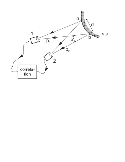
Figure 1: An example of the incorrect view of spectroscopic QS correlations in astronomy gra77 . Neither the extremely small three-momentum difference ${\bf q}$ between the photons from the same emitter (a negligible part of the photon pairs) nor the one between the photons from different emitters can directly be measured in astronomy. In fact, this figure would be a correct view of femtoscopic QS correlations if a distant star were substituted by a nearby object emitting identical particles at a characteristic space-time distance of the order of femtometer.

IV FEMTOSCOPIC FSI CORRELATIONS

It can be shown gkw79 ; ll1 ; led05 that the effect of FSI manifests itself in the fact that the role of functional basis, which the asymptotic two-particle state is projected on, is transferred from plane waves $\exp(-ip_{1}x_{1}-ip_{2}x_{2})$ to the Bethe-Salpeter amplitudes $\Psi_{p_{1}p_{2}}^{(-)}(x_{1},x_{2})=\Psi_{p_{1}p_{2}}^{(+)*}(x_{1},x_{2})=\exp(-iPX)\psi_{\tilde{q}}^{(+)*}(\Delta x)$, where $\Delta x\equiv x_{1}-x_{2}=\{t,{\bf r}\}$ is the relative four-coordinate, $\widetilde{q}=q-P(qP)/P^{2}$ is the generalized relative four-momentum, $P=p_{1}+p_{2}$ and $qP=m_{1}{}^{2}-m_{2}{}^{2}$.

To simplify the calculation of the FSI effect, the Bethe-Salpeter amplitude describing two particles emitted at space-time points $x_{i}=\{t_{i},{\bf r}_{i}\}$ and detected with four-momenta $p_{i}$ is usually calculated at equal emission times in the pair c.m. system; i.e. the reduced non-symmetrized Bethe-Salpeter amplitude $\psi_{{\tilde{q}}}^{(+)}(\Delta x)$ is substituted in the two-particle c.m. system, where ${\bf P}=0$, $\tilde{q}=\{0,2{\bf k}^{*}\}$ and $\Delta x=\{t^{*},{\bf r}^{*}\}$), by a stationary solution $\psi^{(+)}_{-{\bf k}^{*}}({\bf r}^{*})$ of the scattering problem having at large distances ${r}^{*}$ the asymptotic form of a superposition of the plane and outgoing spherical waves (the minus sign of the vector ${\bf k}^{*}$ corresponds to the reverse in time direction of the emission process). This equal time approximation is valid on conditions ll1 ; led05 $|t^{*}|\ll m_{2,1}r^{*2}$ for ${\rm sign}(t^{*})=\pm 1$ respectively. These conditions are usually satisfied for heavy particles like kaons or nucleons. But even for pions, the $t^{*}=0$ approximation merely leads to a slight overestimation (typically $<5\%$) of the strong FSI effect (see figure 2 and led05 ) and, it doesn’t influence the leading zero–distance ($r^{*}\ll|a|$) effect of the Coulomb FSI.

Figure 2: The FSI contribution to the $\pi^{0}\pi^{0}$ correlation function calculated for the pair velocity $v=0.3,0.5,0.7,0.9~{}c$ in a model of independent single–particle emitters distributed according to a Gaussian law with the spatial and time width parameters $r_{0}=2$ fm and $\tau_{0}=2$ fm/$c$. The exact results (solid curves) are compared with those obtained in the equal–time approximation (dash curves).

Note that in the case of small $k^{*}$, we are interested in, the short-range interaction is dominated by central forces and s-waves so that, neglecting a weak spin dependence of the Coulomb interaction, the spin dependence of the two-particle amplitude enters only through the total spin $S$.

On the assumptions (i)-(iv), the two-particle correlation function then reduces to the square of the two-particle wave function averaged over the distance ${\bf r}^{*}$ of the emitters in the two-particle c.m. system and the total spin $S$ of the pair:

$${\cal R}(p_{1},p_{2})\doteq\langle|\psi_{-{\bf k}^{*}}^{(+)}({\bf r}^{*})|^{2}\rangle.$$ (17)

For identical particles, the amplitude in Eq. (17) enters in a symmetrized form:

$$\psi_{-{\bf k}^{*}}^{(+)}({\bf r}^{*})\rightarrow[\psi_{-{\bf k}^{*}}^{(+)}({\bf r}^{*})+(-1)^{S}\psi_{{\bf k}^{*}}^{(+)}({\bf r}^{*})]/\sqrt{2}.$$ (18)

The two-particle approximation in (i) and FSI factorization in the Bethe-Salpeter amplitudes of the elastic transitions $1+2\to 1+2$ implies a long FSI time as compared with the characteristic production time, i.e. the channel momentum $k^{*}$ much less than typical production momentum transfer of hundreds MeV/$c$. In fact, the long-time FSI can be also factorized in the inelastic transitions, $1+2\to 3+4$, characterized by a slow relative motion in both entrance and exit channels lll97 ; led05 . The necessary condition is an approximate equality of the sums of particle masses in the channels $1+2$ and $3+4$. In the presence of such transitions the two-channel scattering problem has to be solved and both elastic and inelastic transition amplitudes should be taken into account in the averaging in Eq. (17). In practice, the particles $1,3$ and $2,4$ are members of the same isomultiplets (as, e.g., in the transition $\pi^{-}p\to\pi^{0}n$ or $K^{+}K^{-}\to K^{0}\bar{K^{0}}$) so that one can assume the same weights and same ${\bf r}^{*}$-distributions for the channels $1+2$ and $3+4$.

In heavy ion collisions, the effective radius $r_{0}$ of the emission region can be considered much larger than the range of the strong interaction potential. The short range FSI contribution to the correlation function is then independent of the actual potential form ll1 ; gkll86 . At small $Q=2k^{*}$, it is determined by the s-wave scattering amplitudes $f^{S}(k^{*})$ at a given total spin $S$ scaled by the radius $r_{0}$ ll1 . For two-nucleon systems, the scattering lengths $f^{S}(0)$ are large (up to $\sim 20$ fm) and this contribution often dominates over the effect of QS. For two-meson or meson-baryon systems, the scattering amplitudes are usually quite small ($<0.2$ fm) and the short range FSI contribution (including the contribution of the coupled channel which is quadratic in the amplitude of the corresponding inelastic transition) can be often neglected. This contribution cannot be however neglected for the $K\bar{K}$-system due to rather large s-wave $K\bar{K}$ scattering length dominated by the imaginary part of $\sim$1 fm generated by near-threshold resonances $f_{0}(980)$ and $a_{0}(980)$ ll1 . It has been recently shown that the neglect of the FSI contribution in the analysis of the two-$K_{S}^{0}$ correlation function in Au+Au collisions at $\sqrt{s}_{NN}=200$ GeV would lead to a noticeable ($\sim 25\%$) overestimation of the correlation radius starksks .

V FEMTOSCOPIC CORRELATIONS IN BETA-DECAY

Let us now consider beta-decay of a nucleus with charge number $Z_{0}$, four-momentum $p_{0}$, helicity $\lambda_{0}$ to a nucleus with charge number $Z$, four-momentum $p$, helicity $\lambda$, an electron (positron) with four-momentum $p_{\rm e}$, helicity $\lambda_{\rm e}$ and an antineutrino (neutrino) with four-momentum $p_{\nu}$, helicity $\lambda_{\nu}$. Taking into account the point-like character of the weak interaction, the equal emission times of the decay particles and the fact that the c.m. system of the electron and final nucleus practically coincides with the rest frame of the initial nucleus (i.e. ${\bf x}_{Z}\doteq{\bf x}_{Z_{0}}=0$ and ${\bf k}^{*}\doteq{\bf p}_{\rm e}$), one can write the differential decay rate in the form:

$$d^{5}w\doteq\sum_{\lambda^{\prime}{\rm s}}\int d^{3}{\bf p}d^{3}{\bf p}_{\rm e}d^{3}{\bf p}_{\nu}\delta^{4}(p_{0}-p-p_{\rm e}-p_{\nu})\cdot$$

$$\cdot\left|\int d^{3}{\bf x}~{}{\cal T}({\bf x};\lambda^{\prime}{\rm s})\exp(i{\bf p}_{\nu}{\bf x})\psi_{-{\bf k}^{*}}^{(+)*}({\bf x})\right|^{2}$$

$$\doteq\sum_{\lambda^{\prime}{\rm s}}\int d^{3}{\bf k}^{*}d^{3}{\bf p}_{\nu}\delta(\omega_{0}-\omega-\omega_{\rm e}-\omega_{\nu})\int d^{3}{\bf x}d^{3}{\bf x}^{\prime}\cdot$$

$$\cdot{\cal T}({\bf x};\lambda^{\prime}{\rm s}){\cal T}^{*}({\bf x}^{\prime};\lambda^{\prime}{\rm s})\exp[i{\bf p}_{\nu}({\bf x}-{\bf x}^{\prime})]\psi_{-{\bf k}^{*}}^{(+)*}({\bf x})\psi_{-{\bf k}^{*}}^{(+)}({\bf x}^{\prime}),\hskip 11.38092pt$$ (19)

where the amplitude ${\cal T}({\bf x};\lambda^{\prime}{\rm s})$ is basically determined by the distribution of the decaying neutron (proton) within the nucleus.

It is instructive to consider the hypothetical situation when the energy release in the decay is large and additional particles are emitted. Then one could neglect the energy-momentum conservation and get, after the integration over the neutrino three-momentum (leading to delta-function $\delta^{3}({\bf x}-{\bf x}^{\prime})$), similar result as in the case of multiparticle production on conditions (i)-(iv):

$$\frac{d^{3}w}{d^{3}{\bf k}^{*}}\propto\int d^{3}{\bf x}\sum_{\lambda^{\prime}{\rm s}}\left|{\cal T}({\bf x};\lambda^{\prime}{\rm s})\psi_{-{\bf k}^{*}}^{(+)*}({\bf x})\right|^{2}\propto\left\langle\left|\psi_{-{\bf k}^{*}}^{(+)}({\bf x})\right|^{2}\right\rangle.$$ (20)

The actual energy release in beta-decay is however very small so that the integration over the neutrino three-momentum does not lead to the diagonalization of the spatial density matrix $\sum_{\lambda^{\prime}{\rm s}}{\cal T}({\bf x};\lambda^{\prime}{\rm s}){\cal T}^{*}({\bf x}^{\prime};\lambda^{\prime}{\rm s})$. In fact, in so-called allowed decays, the neutrino plane wave $\exp(i{\bf p}_{\nu}{\bf x})$ can be even substituted by unity. Nevertheless, similar result as in Eq. (20) has been obtained by Fermi fer34 due to the fact that the relativistic Coulomb wave function $\psi_{-{\bf k}^{*}}^{(+)*}({\bf x})$ of the electron (positron)-nucleus system changes very little within the nucleus and can be taken out of the integral in a form of the so-called Fermi function ${F}(k^{*},Z,R)$. Neglecting the neutrino mass and the nucleus recoil energy (i.e. putting $\omega_{\nu}=|{\bf p}_{\nu}|$ and $\omega=M$), one can write in the nucleus rest frame ($\omega_{0}=M_{0}$):

$$\frac{d^{3}w}{d^{3}{\bf k}^{*}}\doteq 4\pi{F}(k^{*},Z,R)(M_{0}-M-\omega_{e})^{2}\sum_{\lambda^{\prime}{\rm s}}\left|\int d^{3}{\bf x}~{}{\cal T}({\bf x};\lambda^{\prime}{\rm s})\right|^{2},$$ (21)

where

$${F}(k^{*},Z,R)\doteq\langle|\psi_{-{\bf k}^{*}}^{(+)}({\bf r}^{*})|^{2}\rangle\doteq|\psi_{-{\bf k}^{*}}^{(+)}(R)|^{2}$$

$$\hskip 8.5359pt\doteq(2k^{*}R)^{2\sigma}\frac{2\sigma+4}{[\Gamma(2\sigma+3)]^{2}}\exp(-\pi\eta)|\Gamma(\sigma+1-i\eta)|^{2},~{}~{}~{}~{}~{}~{}$$ (22)

$\eta\doteq\mp Ze^{2}\omega_{e}/k^{*}$ for electrons (positrons), $\sigma=(1-Ze^{2})^{1/2}-1$. The substitution of the separation $r^{*}$ by the nucleus radius $R$ in the second equality in Eq. (22) is justified due to a weak $r^{*}$-dependence of the wave function within the nucleus fer34 ; the third equality neglects the screening effect of the atomic electrons.

One may see that the nucleus radius enters in the Fermi function through the factor $(2k^{*}R)^{2\sigma}$ which is essentially different from unity only for sufficiently large charge numbers $Z$. At small $Z$-values, $\sigma\doteq 0$ and the Fermi function reduces to the Coulomb penetration (Gamow) factor $A_{c}(\eta)=|\psi_{-{\bf k}^{*}}^{(+)}(0)|^{2}=2\pi\eta[\exp(2\pi\eta)-1]^{-1}$. The sensitivity of the Fermi function to the nucleus radius is demonstrated in figure 3.

Figure 3: The Fermi function $F(k^{*},Z,R)$ for beta-decay to a final nucleus of charge $Z=83$ as a function of the electron (decreasing curves) or positron momentum $k^{*}$ and the nucleus radius $R=2,4,8$ fm (in decreasing order).

VI Conclusions

We have considered femtoscopic QS and FSI momentum correlations in multiparticle production and beta-decay, as well as spectroscopic QS space-time correlations in the detected radiation from a distant source. We have demonstrated the orthogonal character of the femtoscopic and spectroscopic correlations, earlier pointed out by Kopylov and Podgoretsky KP75 . We have shown that the same functional form of the two-particle correlation function in multiparticle production and Fermi function in beta-decay (both being equal to the average square of the two-particle wave function) is due to different reasons. In former case, this result is valid in the approximation of independent classical quasi-point-like particle emitters and sufficiently small freeze-out phase space density, while in the latter case it follows from a weak variation of the electron (positron)-nucleus wave function within the nucleus volume and a point-like character of beta-decay. It should be stressed that a small space-time extent of the emitters alone does not guarantee the validity of the approximation of classical emitters (the diagonalization of the space-time density matrix). This approximation may naturally be justified in high-energy multiparticle processes due to the minor importance of conservation laws in this case.

Acknowledgements This work was supported by the Grant Agency of the Czech Republic under contract 202/07/0079 and partly carried out within the scope of the GDRE: Heavy ions at ultrarelativistic energies - a European Research Group comprising IN2P3/CNRS, EMN, University of Nantes, Warsaw University of Technology, JINR Dubna, ITEP Moscow and BITP Kiev.

References

- (1) G. Goldhaber, S. Goldhaber, W. Lee and A. Pais, Phys. Rev. 120, 300 (1960).
- (2) V.G. Grishin, G.I. Kopylov and M.I. Podgoretsky, Sov. J. Nucl. Phys. 13, 638 (1971).
- (3) G.I. Kopylov and M.I. Podgoretsky, Sov. J. Nucl. Phys. 15, 219 (1972).
- (4) G.I. Kopylov, Phys. Lett. B50, 472 (1974).
- (5) M.I. Podgoretsky, Sov. J. Part. Nucl. 20, 266 (1989).
- (6) E.V. Shuryak, Phys. Lett. B44, 387 (1973).
- (7) G. Cocconi, Phys. Lett. B49, 459 (1974).
- (8) G.I.Kopylov and M.I.Podgoretsky, Sov. Physics JETP 42, 211 (1975).
- (9) V.L. Lyuboshitz, Proc. CRIS’98, Acicastello, Italy, 1998, p. 213.
- (10) R. Hanbury-Brown and R.Q. Twiss, Nature 178, 1046 (1956).
- (11) M.L. Goldberger, H.W. Lewis and K.M. Watson, Phys. Rev. 142, 25 (1966).
- (12) D.T. Phillips, H. Kleiman and S.P. Davis, Phys. Rev. 153, 113 (1967).
- (13) S.E. Koonin, Phys. Lett. B70, 43 (1977).
- (14) M. Gyulassy, S.K. Kauffmann and L.W. Wilson, Phys. Rev. C20, 2267 (1979).
- (15) R. Lednicky and V.L. Lyuboshitz, Sov. J. Nucl. Phys. 35, 770 (1982); Proc. CORINNE 90, Nantes, France, 1990 (ed. D. Ardouin, World Sci., 1990) p. 42.
- (16) D.H. Boal and J.C. Shillcock, Phys. Rev. C33, 549 (1986).
- (17) D.H. Boal, C.-K. Gelbke and B.K. Jennings, Rev. Mod. Phys. 62, 553 (1990).
- (18) H. Sato and K. Yazaki, Phys. Lett. B98, 153 (1981).
- (19) V.L. Lyuboshitz, Sov. J. Nucl. Phys. 48, 956 (1988).
- (20) S. Mrowczynski, Phys. Lett. B277, 43 (1992); ibid. B308, 216 (1993).
- (21) R. Scheibl and U. Heinz, Phys. Rev. C59, 1585 (1999).
- (22) R. Lednicky, V.L. Lyuboshitz, B. Erazmus and D. Nouais, Phys. Lett. B373, 30 (1996).
- (23) B. Erazmus et al., CERN Note ALICE-INT-1995-43.
- (24) S. Voloshin, R. Lednicky, S. Panitkin and N. Xu, Phys. Rev. Lett. 79, 4766 (1997).
- (25) D. Ardouin et al., Phys. Lett. B446, 191 (1999).
- (26) R. Lednicky, S. Panitkin and N. Xu, nucl-th/0304062.
- (27) R. Lednicky, nucl-th/0304063, 0304064.
- (28) D. Miskowiec et al. (E877), nucl-ex/9808003.
- (29) R. Lednicky, NA49 Note number 210 (1999); nucl-th/0112011, 0212089.
- (30) Ch. Blume et al. (NA49), Nucl. Phys. A715, 55c (2003).
- (31) J. Adams et al. (STAR), Phys. Rev. Lett. 91, 262302 (2003).
- (32) A. Kisiel (STAR), J. Phys. G30, S1059 (2004).
- (33) R. Lednicky, Phys. Atom. Nucl. 67, 72 (2004).
- (34) E. Fermi, Z. Phys. 88, 161 (1934); F.L. Wilson, Am. J. Phys. 36, 1150 (1968).
- (35) M. Lisa, S. Pratt, R. Soltz and U. Wiedemann, Ann. Rev. Nucl. Part. Sci. 55, 357 (2005).
- (36) T. Csörgő, nucl-th/0505019.
- (37) R. Lednicky, Nucl. Phys. A774, 189 (2006).
- (38) Yu.M. Sinyukov, R. Lednicky, S.V. Akkelin, J. Pluta and B. Erazmus, Phys. Lett. B432, 248 (1998).
- (39) R. Lednicky and T.B. Progulova, Z. Phys. C55, 295 (1992).
- (40) R. Lednicky and V.L. Lyuboshitz, Heavy Ion Physics 3, 93 (1996).
- (41) S. Cheng and S. Pratt, Phys. Rev. C63, 054904 (2001).
- (42) D. Neuhauser, Phys. Lett. B182, 289 (1986).
-
(43)
V.L. Lyuboshitz, M.I. Podgoretsky, Phys. Atom. Nucl. 58, 30
(1995); V.L. Lyuboshitz, http://www.itep.ru/ions/GDRE/Dubna -ITEP-March-2006/GDRE_Dubna_Itep_March2006.html. - (44) V.L. Lyuboshitz, M.I. Podgoretsky, Sov. J. Nucl. Phys. 30, 407 (1979).
- (45) S. Pratt, Phys. Rev. Lett. 53, 1219 (1984); Phys. Rev. D33, 1314 (1986); S. Pratt, T. Csörgö and J. Zimanyi, Phys. Rev. C42, 2646 (1990).
- (46) A.N. Makhlin and Yu.M. Sinyukov, Yad. Fiz. 46, 637 (1987); Z. Phys. C39, 69 (1988); Yu.M. Sinyukov, Nucl. Phys. A498, 151c (1989).
- (47) U.A. Wiedemann and U. Heinz, Phys. Rept. 319, 145 (1999).
- (48) T. Csörgö, Heavy Ion Phys. 15, 1 (2002).
- (49) M.I. Podgoretsky, Sov. J. Nucl. Phys. 37, 272 (1983); R. Lednicky, JINR B2-3-11460, Dubna (1978); P. Grassberger, Nucl. Phys. B120, 231 (1977).
- (50) G.F. Bertsch, P. Danielewicz and M. Herrmann, Phys. Rev. C49, 442 (1994); S. Pratt, in Quark Gluon Plasma 2 (ed. R.C. Hwa), World Scientific, Singapore, 1995, p.700; S. Chapman, P. Scotto and U. Heinz, Phys. Rev. Lett. 74, 4400 (1995).
- (51) U.A. Wiedemann, Phys. Rev. C57, 266 (1998).
- (52) T. Csörgö and S. Pratt, Proc. Workshop on Heavy Ion Physics, KFKI-1991-28/A, p.75.
- (53) P. Grassberger, Proc. VIII-th International Symposium on Multiparticle Dynamics, Kaysersberg, France, June 12-17, 1977.
- (54) W. Bauer, C-K. Gelbke and S. Pratt, Annu. Rev. Nucl. Part. Sci 42, 77 (1992).
- (55) R. Lednicky, nucl-th/0501065.
- (56) R. Lednicky, V.V. Lyuboshitz and V.L. Lyuboshitz, Phys. Atom. Nucl. 61, 2050 (1998).
- (57) M. Gmitro, J. Kvasil, R. Lednicky and V.L. Lyuboshitz, Czech. J. Phys. B36, 1281 (1986).
- (58) B. I. Abelev et al. (STAR), Phys. Rev. C74, 054902 (2006).