Momentum distributions and spectroscopic factors of doubly-closed shell nuclei in correlated basis function theory

Abstract

The momentum distributions, natural orbits, spectroscopic factors and quasi-hole wave functions of the ¹²C ,¹⁶O ,⁴⁰Ca ,⁴⁸Ca , and ²⁰⁸Pb doubly closed shell nuclei, have been calculated in the framework of the Correlated Basis Function theory, by using the Fermi hypernetted chain resummation techniques. The calculations have been done by using the realistic Argonne $v^{\prime}_{8}$ nucleon-nucleon potential, together with the Urbana IX three-body interaction. Operator dependent correlations, which consider channels up to the tensor ones, have been used. We found noticeable effects produced by the correlations. For high momentum values, the momentum distributions show large enhancements with respect to the independent particle model results. Natural orbits occupation numbers are depleted by about the 10% with respect to the independent particle model values. The effects of the correlations on the spectroscopic factors are larger on the more deeply bound states.

I INTRODUCTION

One of the major achievements of nuclear structure studies in the last ten years is the consolidation of the validity of the non relativistic many-body approach. The idea is to describe the nucleus with a Hamiltonian of the type:

$$H=-\frac{\hbar^{2}}{2m}\sum_{i}^{A}\nabla_{i}^{2}+\sum_{i<j=1}^{A}v_{ij}+\sum_{i<j<k=1}^{A}v_{ijk}\,\,,$$ (1)

where the two- and three-body interactions, $v_{ij}$ and $v_{ijk}$ respectively, are fixed to reproduce the properties of the two- and three-body nuclear systems. The Schrödinger equation has been solved without approximations for few body systems Kamada et al. (2001) and light nuclei Pudliner et al. (1997), up to A=12 Pieper (2005). The obtained results provide good descriptions, not only of the energies of these nuclei, but also of other observables.

The difficulties in extending to medium and heavy nuclei the techniques used in few body systems and light nuclei, favored the development of models, and of effective theories. The basic idea of the effective theories is to work in a restricted space of the many-body wave functions. Usually, one works with many-body wave functions which are Slater determinants of single particle wave functions. The idea of single particle wave functions implies the hypothesis of a mean-field where each nucleon move independently from the other ones. This Independent Particle Model (IPM) is quite far from the picture outlined by the microscopic calculations quoted above, describing the nucleus as a many-body system of strongly interacting nucleons. In the Hartree-Fock theory, which provides the microscopic foundation of the IPM, the Hamiltonian is not any more that of Eq. (1), but it is an effective Hamiltonian built to take into account, obviously in an effective manner, the many-body effects that the microscopic calculations explicitly consider. The construction of effective interactions starting from the microscopic ones, covers a wide page of the nuclear physics history, starting from the Brueckner G-matrix effective interactions Brueckner (1955); Nakayama et al. (1985), up to the recent $V_{lowk}$ interaction Bogner et al. (2003); Coraggio et al. (2006) and the interaction obtained by applying the unitary correlation operator method Roth et al. (2004, 2006).

The application of the IPM is quite successful, but there are evidences of the intrinsic limitations in its applicability. For example, the measured spectroscopic factors are systematically smaller than one Lapikás (1993); Kramer et al. (2001); van Batenburg (2001), which is the value predicted by the IPM. The (e,e’p) cross sections in the quasi-elastic region need a consistent reduction of the IPM hole strength to be explained Quint (1988); Boffi et al. (1996). The same holds for the electromagnetic form factors of the low-lying states, especially those having large angular momentum Lichtenstadt et al. (1979); Hyde-Wright et al. (1987). The emission of two like nucleons in photon and electron scattering process cannot be described by the IPM Onderwater et al. (1997, 1998). Also the charge density distributions extracted by elastic electron scattering data are, in the nuclear interior, smaller than those predicted by the IPM Cavedon et al. (1982); Papanicolas (1986). These examples indicate the presence of physics effects, commonly called correlations, which are not described by the IPM.

It is common practice to distinguish between long- and short-range correlations since they have different physical sources. The long-range correlations are related to collective excitations of the system, such as the giant resonances. The short-range correlations (SRC) are instead connected to the strongly repulsive core of the microscopic nucleon-nucleon interaction. The repulsive core reduces the possibility that two nucleons can approach each other, and this modifies the IPM picture where, by definition, the motion of each nucleon does not depend on the presence of the other ones.

Even though most of the calculations of medium heavy nuclei are based on the IPM, and on the effective theories, various techniques, aiming to attack the problem by using the microscopic Hamiltonian (1), have been developed. The Brueckner-Hartree-Fock approach has been recently applied to the ¹⁶O nucleus Dickhoff and Barbieri (2004). No core-shell model calculations have been done for nuclei lighter than ¹²C Navrátil et al. (2000); Forssén et al. (2005). The coupled cluster method has been used to evaluate ¹⁶O properties Heisenberg and Mihaila (1999); Mihaila and Heisenberg (1999).

About fifteen years ago Co’ et al. (1992), we started a project aimed to apply to the description of medium and heavy nuclei the Correlated Basis Function (CBF) theory, successfully used to describe the nuclear and neutron matter properties Wiringa et al. (1988); Akmal et al. (1998). We solve the many-body Schrödinger equation by using the variational principle:

$$\delta E[\Psi]=\delta\frac{<\Psi|H|\Psi>}{<\Psi|\Psi>}=0\,\,.$$ (2)

The search for the minimum of the energy functional is done within a subspace of the full Hilbert space spanned by the A-body wave functions which can be expressed as:

$$\Psi(A)={\cal F}(1,...,A)\Phi(1,...,A)\,\,,$$ (3)

where ${\cal F}(1,...,A)$ is a many-body correlation operator and $\Phi(1,...,A)$ is a Slater determinant composed by single particle wave functions, $\phi_{\alpha}(i)$. In our calculations, we used two-body interactions of Argonne and Urbana type, and we considered all the interaction channels up to the spin-orbit ones. Together with these two-body interactions, we used the appropriated three-body forces of Urbana type. The complexity of the interaction required the use of operator dependent correlations. We consider correlations of the type:

$${\cal F}={\cal S}\left(\prod_{i<j=1}^{A}F_{ij}\right)\,\,,$$ (4)

where ${\cal S}$ is a symmetrizer operator and $F_{ij}$ is expressed in terms of two-body correlation functions $f_{p}$ as:

$$F_{ij}=\sum_{p=1}^{6}f_{p}(r_{ij})O^{p}_{ij}\,\,.$$ (5)

In the above equation we have adopted the nomenclature commonly used in this field, by defining the operators as:

$$O^{p=1,6}_{ij}=[1,\mbox{\boldmath$\sigma$}_{i}\cdot\mbox{\boldmath$\sigma$}_{j},S_{ij}]\otimes[1,\mbox{\boldmath$\tau$}_{i}\cdot\mbox{\boldmath$\tau$}_{j}]\,\,,$$ (6)

where $\mbox{\boldmath$\sigma$}_{i}$ and $\mbox{\boldmath$\tau$}_{i}$ indicate the usual Pauli spin and isospin operators, and $S_{ij}=(3\hat{{\bf r}}_{ij}\cdot\mbox{\boldmath$\sigma$}_{i}\hat{{\bf r}}_{ij}\cdot\mbox{\boldmath$\sigma$}_{j}-\mbox{\boldmath$\sigma$}_{i}\cdot\mbox{\boldmath$\sigma$}_{j})$ is the tensor operator.

We recently succeeded in formulating the Fermi Hypernetted Chain (FHNC) equations, in Single Operator Chain (SOC) approximation, for nuclei non saturated in isospin, and with single particle basis described in a $jj$ coupling scheme. We presented in Ref. Bisconti et al. (2006) the binding energies and the charge distributions of ¹²C , ¹⁶O , ⁴⁰Ca , ⁴⁸Ca and ²⁰⁸Pb doubly closed shell nuclei obtained by using the minimization procedure (2). These calculations have the same accuracy of the best variational calculations done in nuclear and neutron matter Wiringa et al. (1988); Akmal et al. (1998).

In the present article, we show the results of our study, done in the FHNC/SOC computational scheme, on some ground state quantities related to observables. They are momentum distributions, natural orbits and their occupation numbers, quasi-hole wave functions and spectroscopic factors. We used the many-body wave functions obtained in Ref. Bisconti et al. (2006) by solving Eq. (2) with the Argonne $v^{\prime}_{8}$ two-nucleon potential, together with the Urbana IX three-body force. We have calculated momentum distributions also with the wave functions produced by another interaction, the Urbana $v_{14}$ truncated up to the spin-orbit terms, implemented with the Urbana VII three-body force. The results obtained with this last interaction do not show relevant differences with those obtained with the $v^{\prime}_{8}$ and UIX interaction, therefore we do not present them.

The paper is organized as follows. In Sect. II we present the results of the One-Body Density Matrix (OBDM) and of the momentum distribution. In Sect. III we discuss the natural orbits, i.e. the single particle wave functions forming the basis where the OBDM is diagonal. In Sect. IV we present our results about the quasi-hole wave functions and in Sect. V we summarize our results and draw our conclusions.

II ONE-BODY DENSITY MATRIX AND MOMENTUM DISTRIBUTION

We define the one-body density matrix, (OBDM), of a system of $A$ nucleons as:

$$\rho(x_{1},x^{\prime}_{1}) \equiv \sum_{s,s^{\prime},t}\rho^{s,s^{\prime};t}({\bf r}_{1},{\bf r}^{\prime}_{1})\,\chi^{\dagger}_{s}(1)\chi^{\dagger}_{t}(1)\chi_{s^{\prime}}(1^{\prime})\chi_{t}(1^{\prime})$$ (7)

$$\equiv \frac{A}{<\Psi|\Psi>}\int dx_{2}\ldots dx_{A}\Psi^{\dagger}(x_{1},x_{2},\ldots,x_{A})\Psi(x^{\prime}_{1},x_{2},\ldots,x_{A})\,\,\,.$$

In the above expression, the variable $x_{i}$ indicates the position (${\bf r}_{i}$) and the third components of the spin ($s_{i}$) and of the isospin ($t_{i}$) of the single nucleon. The $\chi(i)$ functions represent the Pauli spinors. With the integral sign we understand that also the sum on spin and isospin third components of all the particles from 2 up to A, is done. In our calculations we are interested in the quantity:

$$\rho^{t}({\bf r}_{1},{\bf r}^{\prime}_{1})=\sum_{s=\pm 1/2}\left[\rho^{s,s;t}({\bf r}_{1},{\bf r}^{\prime}_{1})+\rho^{s,-s;t}({\bf r}_{1},{\bf r}^{\prime}_{1})\right]\,\,,$$ (8)

whose diagonal part (${\bf r}^{\prime}_{1}={\bf r}_{1}$) represents the one-body density of neutrons or protons.

We obtain the momentum distributions of protons ($t$=1/2) or neutrons ($t$=-1/2) as:

$$n^{t}(k)=\frac{1}{(2\pi)^{3}}\frac{1}{{\cal N}_{t}}\int d{\bf r}_{1}d{\bf r}^{\prime}_{1}\,e^{i{\bf k}\cdot({\bf r}_{1}-{\bf r}^{\prime}_{1})}\rho^{t}({\bf r}_{1},{\bf r}^{\prime}_{1})\,\,,$$ (9)

where we have indicated with ${\cal N}_{t}$ the number of protons or neutrons. The above definitions imply the following normalization of $n(k)$:

$$\int d{\bf k}\,n^{t}(k)=1\,\,.$$ (10)

We describe doubly closed shell nuclei, with different numbers of proton and neutrons, in a $jj$ coupling scheme. The most efficient single particle basis to be used is constructed by a set of single particle wave functions expressed as:

$$\phi^{t}_{nljm}({\bf r}_{i})=R^{t}_{nlj}(r_{i})\sum_{\mu,s}<l\mu\frac{1}{2}s|jm>Y_{l\mu}(\Omega_{i})\chi_{s}(i)\chi_{t}(i)=R^{t}_{nlj}(r_{i}){\bf Y}^{m}_{lj}(\Omega_{i})\chi_{t}(i)\,\,.$$ (11)

In the above expression we have indicated with $Y_{l\mu}$ the spherical harmonics, with $<|>$ the Clebsch-Gordan coefficient, with $R^{t}_{nlj}(r_{i})$ the radial part of the wave function, and with ${\bf Y}^{m}_{lj}$ the spin spherical harmonics Edmonds (1957).

The uncorrelated OBDMs, those of the IPM, are obtained by substituting in Eq. (7) the correlated function $|\Psi>$ with the Slater determinant $|\Phi>$ formed by the single particle wave functions (11). We obtain the following expressions:

$$\rho_{o}^{t}({\bf r}_{1},{\bf r}^{\prime}_{1})=\sum_{s}\left[\rho_{o}^{s,s;t}({\bf r}_{1},{\bf r}^{\prime}_{1})+\rho_{o}^{s,-s;t}({\bf r}_{1},{\bf r}^{\prime}_{1})\right]\,\,,$$

$$\rho_{o}^{s,s;t}({\bf r}_{1},{\bf r}^{\prime}_{1}) = \frac{1}{8\pi}\sum_{nlj}(2j+1)R^{t}_{nlj}(r_{1})R^{t}_{nlj}(r^{\prime}_{1})P_{l}(\cos\theta_{11^{\prime}})\,\,,$$ (12)

$$\rho_{o}^{s,-s;t}({\bf r}_{1},{\bf r}^{\prime}_{1}) = \frac{1}{4\pi}\sum_{nlj}(-1)^{j-l-1/2}R^{t}_{nlj}(r_{1})R^{t}_{nlj}(r^{\prime}_{1})\sin\theta_{11^{\prime}}P^{\prime}_{l}(\cos\theta_{11^{\prime}})\,\,.$$ (13)

In the above equations $\theta_{11^{\prime}}$ indicates the angle between ${\bf r}_{1}$ and ${\bf r}^{\prime}_{1}$, and $P_{l}$ and $P^{\prime}_{l}$ the Legendre polynomials and their first derivative respectively. The presence of the second term of Eq. (II), the antiparallel spin terms given in Eq. (13), is due the $jj$ coupling scheme required to describe heavy nuclei.

The correlated OBDM is obtained by using the ansatz (3) in Eq. (7). This calculation is done by using the cluster expansion techniques as indicated in Co’ et al. (1994) and de Saavedra et al. (1996), where only scalar correlations have been used, and in Fabrocini and Co’ (2001), where the state dependent correlations have been used, but in a $ls$ coupling scheme. We followed the lines of Ref. Fabrocini and Co’ (2001) and, in addition, we consider the presence of the antiparallel spin terms and we distinguish proton and neutron contributions. The explicit expression of the OBDM, in terms of FHNC/SOC quantities, such as two-body density distributions, vertex corrections, nodal diagrams etc., is given in Appendix A. The diagonal part of the OBDM is the one-body density, normalized to the number of nucleons. Because of this, the momentum distribution satisfies the following sum rule:

$$S^{t}_{2}=\frac{\hbar^{2}}{2m}\int d{\bf k}\,k^{2}\,n^{t}(k)/T_{FHNC}^{t}=1\,\,,$$ (14)

where we have indicated with $T_{FHNC}^{t}$ the kinetic energy of the protons or of the neutrons. We have verified the accuracy of our calculations by testing the normalization (10) and the exhaustion of the above sum rule for every $n^{t}(k)$ calculated. We found that these quantities are always satisfied at the level of few parts on a thousand in a full FHNC/SOC calculation, and even better when only scalar correlations are used.

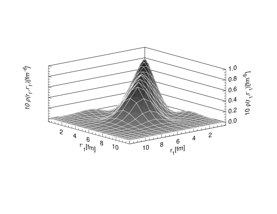
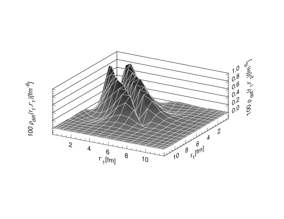
Figure 1: The proton one-body density matrix, $\rho(r_{1},r^{\prime}_{1})$, for the ²⁰⁸Pb nucleus in FHNC/SOC approximation, calculated for $\theta_{11^{\prime}}$=0. The diagonal part $\rho(r_{1},r_{1})$ is the proton density distribution.

Figure 2: The difference $\rho_{o}(r_{1},r^{\prime}_{1})-\rho(r_{1},r^{\prime}_{1})$, between the proton IPM one-body density matrix of the ²⁰⁸Pb nucleus, and that obtained with our FHNC/SOC calculations. The two density matrices, have been calculated for $\theta_{11^{\prime}}$=0. Note that the scale here is ten times larger than that of Fig. 2.

The surface shown in Fig.2 represents the proton OBDM of the ²⁰⁸Pb nucleus, for $\theta_{11^{\prime}}$=0. We have shown in Bisconti et al. (2006) that the SRC lower the one-body proton distribution, and also that of the neutrons, in the nuclear center. In order to highlight the effects of the correlations on the density matrix, we show in Fig. 2 the quantity $\rho_{o}(r_{1},r^{\prime}_{1})-\rho(r_{1},r^{\prime}_{1})$. Note that the $z$-axis scale of Fig. 2 is ten times larger than that of Fig.2. It is interesting to notice that the major differences between the OBDMs are not in the diagonal part, but just beside it. The consequences of these, small, differences between the OBDMs on the momentum distributions, are shown in Fig. 3. In this figure, we compare the ¹²C , ¹⁶O , ⁴⁰Ca , ⁴⁸Ca and ²⁰⁸Pb proton momentum distributions calculated in the IPM model, with those obtained by using scalar and operator dependent correlations.

Figure 3: The proton momentum distributions of the ¹²C , ¹⁶O , ⁴⁰Ca , ⁴⁸Ca and ²⁰⁸Pb nuclei calculated in the IPM model, by using the scalar correlations only ($f_{1}$) and the full operator dependent correlations ($f_{6}$).

Figure 4: The proton momentum distributions of the ¹⁶O and ²⁰⁸Pb nuclei multiplied by $k^{2}$. The full lines show the IPM results, the dotted lines have been obtained by using scalar correlations only, and the dashed lines with the complete correlation.

Figure 5: In the panels (a) and (b) we show the protons (full lines) and neutrons (dashed lines) momentum distributions of the ⁴⁸Ca and ²⁰⁸Pb . The thick lines show the results of our calculations, the thin lines the IPM results. In the panels (c) and (d), we show the weighted difference (15) between uncorrelated and correlated momentum distributions. As in the upper part of the figure, the full lines show the protons results and the dashed lines those of the neutrons.

Figure 6: Proton momentum distribution of ¹⁶O in various approximations. The thick lines are those of the analogous panel of Fig. 3. The thin lines have been obtained by using the first-order expansion method of Ref. de Saavedra et al. (1997).

The general behavior of the momentum distributions, is very similar for all the nuclei we have considered. Correlated and IPM distributions almost coincide in the low momentum region up to a precise value, when they start to deviate. The correlated distributions show high momentum tails, which are orders of magnitude larger than the IPM results. The value of $k$ where uncorrelated and correlated momentum distributions start to deviate, is smaller the heavier is the nucleus. It is about 1.9 fm^-1 for ¹²C , and 1.5 fm^-1 for ²⁰⁸Pb . We notice that the value of the Fermi momentum of symmetric nuclear matter at the saturation density is 1.36 fm^-1.

The results presented in Fig. 3 clearly show that the effects of the scalar correlations are smaller than those obtained by including the operator dependent terms. We shall see in the following that this is a common feature of our results.

Since relatively small differences are compressed in logarithmic scale, we use the linear scale in Fig. 4 to show, as examples, the proton momentum distributions for ¹⁶O and ²⁰⁸Pb nuclei, multiplied by $k^{2}$. This quantity, multiplied by a factor $4\pi$, is the probability of finding a proton with momentum $k$. We observe that the effects of the SRC on the quantity shown in Fig. 4 are basically two. The first one is the already mentioned enhancement at large values of $k$. This effect is less evident here than in Fig. 3. The second effect, hardly visible in Fig. 3, is a reduction of the maxima which appear approximately at $k$=1 fm^-1 in both nuclei. These two effects are obviously related, since all the momentum distributions are normalized as indicated by Eq. (10), therefore reductions and increases must compensate.

We found that the proton and neutron momentum distributions for nuclei with $N=Z$ are very similar. For this reason we do not show the neutron momentum distributions of the ¹²C , ¹⁶O and ⁴⁰Ca nuclei. We compare in the panels (a) and (b) of Fig. 5 the proton and neutron momentum distributions of ⁴⁸Ca and ²⁰⁸Pb . The thicker lines show the results of our FHNC/SOC calculation, the thinner lines the IPM momentum distributions.

The figure shows that, in our calculations, the differences between protons and neutrons momentum distributions are more related to the different single particle structure than to the correlation effects. The main differences in the two distributions is in the zone where the $n(k)$ values drops of orders of magnitudes. This corresponds to the discontinuity region of the momentum distribution in the infinite systems, which is related to the Fermi momentum. In a finite system, the larger number of neutrons implies that the neutron Fermi energy is larger than that of the protons, and, consequently, the effective Fermi momentum. For this reason, the neutrons momentum distributions drops at larger values of $k$ than the proton distributions. In the panels (c) and (d) of Fig. 5, we show the quantity

$$\Delta=\frac{n^{t}_{0}(k)-n^{t}(k)}{n^{t}_{0}(k)+n^{t}(k)}\,\,,$$ (15)

where $n^{t}_{0}(k)$ indicates the uncorrelated momentum distribution. This quantity is useful to point out the effects of correlations. We see that in the low $k$ region $\Delta$ is almost zero. After the discontinuity region $\Delta$ reaches an almost constant value around minus one. This behavior indicates that in the low $k$ region the momentum distribution is dominated by single particle dynamics. The differences between protons and neutrons at low $k$ are due to different single particle wave functions. In the higher $k$ region the correlation plays an important role. We observe that protons and neutrons $\Delta$ are very similar, and this indicate that the effect of the SRC is essentially the same for both kinds of nucleons. Our results are in agreement with the findings of Ref. Bożek (2004), where $n(k)$ of asymmetric nuclear matter is presented. There is however a disagreement with the results of Ref. Frick et al. (2005), where, always in asymmetric nuclear matter, correlations effects between protons were found to be stronger than those between neutrons.

The increase of the momentum distribution at large $k$ values, induced by the SRC is a well known result in the literature, see for example the review of Ref. Antonov et al. (1988). The momentum distributions of medium-heavy nuclei, have been usually obtained by using approximated descriptions of the cluster expansion, which is instead considered at all orders in our treatment. The importance of a complete description of the cluster expansion is exemplified in Fig. 6, where, together with our results, we also show the results of Ref. de Saavedra et al. (1997), obtained by truncating the cluster expansion to the first order in the correlation lines. In both calculations the same correlation functions and single particle basis, those of Ref. Bisconti et al. (2006), have been used. The results obtained with the first order approximation, provide only a qualitative description of the correlation effects. They show high-momentum enhancements which, however, underestimate the correct results by orders of magnitude.

III NATURAL ORBITS

The natural orbits are defined as those single particle wave functions forming the basis where the OBDM is diagonal:

$$\rho^{t}({\bf r}_{1},{\bf r}^{\prime}_{1})=\sum_{nlj}c_{nlj}^{t}\phi_{nlj}^{*\,t,NO}({\bf r}_{1})\phi_{nlj}^{t,NO}({\bf r}^{\prime}_{1})\,\,.$$ (16)

In the above equation the $c^{t}_{nlj}$ coefficients, called occupation numbers, are real numbers. In the IPM, the natural orbits correspond to the mean-field wave functions of Eq. (11), and the $c^{t}_{nlj}$ numbers are 1, for the states below the Fermi surface, and 0 for those above it.

In order to obtain the natural orbits, we found convenient to express the OBDM of Eq. (16) as:

$$\rho^{t}({\bf r}_{1},{\bf r}_{1^{\prime}})=A^{t}({\bf r}_{1},{\bf r}_{1^{\prime}})\rho_{o}^{t}({\bf r}_{1},{\bf r}_{1^{\prime}})+B^{t}({\bf r}_{1},{\bf r}_{1^{\prime}})\,\,,$$ (17)

where $\rho^{t}_{o}({\bf r}_{1},{\bf r}_{1^{\prime}})$ is the uncorrelated OBDM of Eq. (II), and the other two quantities are defined as:

$$A^{t}({\bf r}_{1},{\bf r}^{\prime}_{1}) = 2C_{\omega,SOC}^{t}({\bf r}_{1})C_{\omega,SOC}^{t}({\bf r}^{\prime}_{1})\exp[{N_{\omega\omega}^{t}({\bf r}_{1},{\bf r}^{\prime}_{1})}]+$$ (18)

$$2C_{\omega}^{t}({\bf r}_{1})C_{\omega}^{t}({\bf r}^{\prime}_{1})\exp[{N_{\omega\omega}^{t}({\bf r}_{1},{\bf r}^{\prime}_{1})}]\sum_{p>1}A^{k}\Delta^{k}N_{\omega\omega,p}^{t}({\bf r}_{1},{\bf r}^{\prime}_{1})\,\,,$$

$$B^{t}({\bf r}_{1},{\bf r}^{\prime}_{1}) = -2C_{\omega,SOC}^{t}({\bf r}_{1})C_{\omega,SOC}^{t}({\bf r}^{\prime}_{1})\exp[{N_{\omega\omega}^{t}({\bf r}_{1},{\bf r}^{\prime}_{1})}]N_{\omega_{c}\omega_{c}}^{t}({\bf r}_{1},{\bf r}^{\prime}_{1})-$$ (19)

$$2C_{\omega}^{t}({\bf r}_{1})C_{\omega}^{t}({\bf r}^{\prime}_{1})\exp{[N_{\omega\omega}^{t}({\bf r}_{1},{\bf r}^{\prime}_{1})]}$$

$$\times\sum_{p>1}A^{k}\Delta^{k}\Big{\{}N_{\omega\omega,p}^{t}({\bf r}_{1},{\bf r}^{\prime}_{1})N_{\omega_{c}\omega_{c}}^{t}({\bf r}_{1},{\bf r}^{\prime}_{1})+N_{\omega_{c}\omega_{c},p}^{t}({\bf r}_{1},{\bf r}^{\prime}_{1})\Big{\}}\,\,.$$

The meaning of the $\omega\omega$, $\omega_{c}\omega_{c}$ labels used in the above equations have been defined in Fabrocini and Co’ (2001) where the index $k$ has been defined as $p=2k+l-1$ with $l=0,1$ and $p=1,\ldots,6$. The detailed expressions of the vertex corrections $C$ and of the nodal functions $N$ are given in Appendix A.

We expand the OBDM on a basis of spin spherical harmonics ${\bf Y}^{m}_{lj}$ , Eq. (11),

$$\rho^{t}({\bf r}_{1},{\bf r}^{\prime}_{1})=\sum_{ljm}\frac{1}{2j+1}\left[{\cal A}_{lj}^{t}(r_{1},r^{\prime}_{1})+{\cal B}_{lj}^{t}(r_{1},r^{\prime}_{1})\right]{\bf Y}^{*m}_{lj}(\Omega_{1}){\bf Y}^{m}_{lj}(\Omega^{\prime}_{1})$$ (20)

where $\Omega_{1}$ and $\Omega^{\prime}_{1}$ indicate the polar angles identifying ${\bf r}_{1}$ and ${\bf r}^{\prime}_{1}$. The explicit expressions of the ${\cal A}$ and ${\cal B}$ coefficients are:

$${\cal A}_{lj}^{t}(r_{1},r^{\prime}_{1}) = (2l+1)\sum_{n_{2}l_{2}j_{2}l}(2l_{2}+1)(2j_{2}+1)\left(\begin{array}[]{ccc}l&l_{1}&l_{2}\\ 0&0&0\end{array}\right)^{2}\left\{\begin{array}[]{ccc}j_{2}&l_{1}&j\\ l&1/2&l_{2}\end{array}\right\}^{2}$$ (25)

$$R^{t}_{nl_{2}j_{2}}(r_{1})R^{t}_{nl_{2}j_{2}}(r_{2})A^{t}_{l_{1}}(r_{1},r^{\prime}_{1})$$ (26)

with

$$A_{l}^{t}(r_{1},r^{\prime}_{1})=\frac{2}{2l+1}\int d\Omega A^{t}({\bf r}_{1},{\bf r}^{\prime}_{1})P_{l}(\cos\theta_{11^{\prime}})$$ (27)

and

$${\cal B}_{lj}^{t}(r_{1},r^{\prime}_{1})=\frac{4\pi}{2l+1}\int d(\cos\theta_{11^{\prime}})B^{t}({\bf r}_{1},{\bf r}^{\prime}_{1})P_{l}(\cos\theta_{11^{\prime}})$$ (28)

In the above equations we have used the 3j and 6j Wigner symbols Edmonds (1957). The term ${\cal A}$ depends on both orbital and total angular momenta of the single particle, $l$ and $j$ respectively, and the term ${\cal B}$ depends only on the orbital angular momentum $l$.

As it has been done in Refs. Lewart et al. (1998) and Polls et al. (1995) we identify the various natural orbit with a number, $\alpha$, ordering them with respect to the decreasing value of the occupation probability. The general behavior of our results is analogous to that described in Ref. Lewart et al. (1998) where a system of ³He drops composed by 70 atoms have been studied. The orbits corresponding to states below the Fermi level in the IPM picture, have occupation numbers very close to unity for $\alpha=1$, and very small in all the other cases.

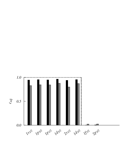
Figure 7: Occupation numbers of the proton natural orbits of the ⁴⁸Ca nucleus, having $\alpha=1$. The dashed line indicates the IPM values. The black bars show the values obtained with the scalar correlation and the gray bars those values obtained with the full correlation.

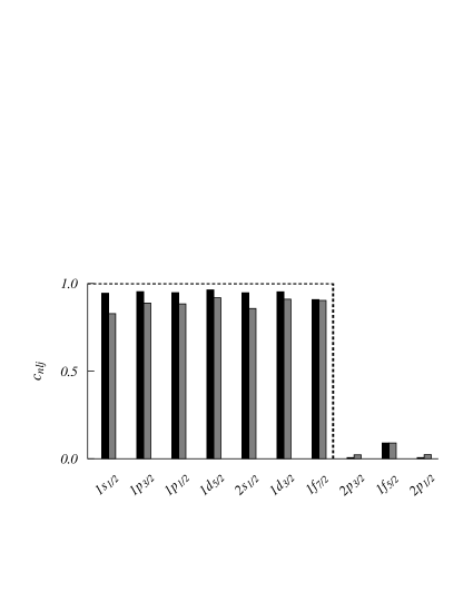
Figure 8: The same as Fig. 7 for the occupation numbers of the neutron natural orbits of the ⁴⁸Ca nucleus.

As example of our results, we show in Figs. 7 and 8 the proton and neutron occupation numbers for the natural orbits with$\alpha=1$ of the ⁴⁸Ca nucleus. In the figures, the IPM results are indicated by the dashed lines. The black bars show the values obtained by using scalar correlations only, the gray bars those obtained with the complete operator dependent correlations.

The correlated occupation numbers are smaller than one for orbits below the Fermi surface, and larger than zero for those orbits above the Fermi surface. This effect is enhanced by the operator dependent correlations. We observe that, for the states above the Fermi surface, the gray bars are larger than the black ones, indicating that also for these states the operator dependent correlations, produce larger effects than the scalar ones.

We show in Fig. 9 some $\alpha=1$ natural orbits for three neutron states in ⁴⁸Ca . In this figure, we compare the IPM results (full lines) with those obtained with scalar correlation only (dotted lines), and with the full operator dependent correlation (dashed lines). The effect of the correlations is a lowering of the peak and a small widening of the function. Despite the small effect, it is interesting to point out that this is the only case where we found that the inclusion of operator dependent terms diminishes the effect of the scalar correlation. This fact is coherent with the results on the density distributions shown in Ref. Bisconti et al. (2006).

State		$\alpha=1$			$\alpha=2$			$\alpha=3$
	$f_{1}$	$f_{6}$	PMD	$f_{1}$	$f_{6}$	PMD	$f_{1}$	$f_{6}$	PMD
$1s_{1/2}$ (p)	0.956	0.873	0.921	0.011	0.038	0.013	0.002	0.007	0.002
(n)	0.957	0.873		0.012	0.039		0.003	0.008
$1p_{3/2}$ (p)	0.973	0.921	0.947	0.004	0.013	0.007	0.001	0.003	0.001
(n)	0.973	0.924		0.004	0.014		0.002	0.004
$1p_{1/2}$ (p)	0.970	0.923	0.930	0.003	0.012	0.008	0.001	0.003	0.002
(n)	0.970	0.922		0.004	0.013		0.002	0.003
$1d_{5/2}$ (p)	0.001	0.005	0.016	0.013	0.003	0.003	0.000	0.000	0.000
(n)	0.001	0.005		0.001	0.003		0.000	0.000
$1d_{3/2}$ (p)	0.002	0.005	0.019	0.001	0.003	0.005	0.000	0.000	0.001
(n)	0.001	0.005		0.001	0.003		0.000	0.000

Table 1: Protons (p) and neutrons (n) natural orbits occupation numbers for ¹⁶O . The PMD values are those of Ref. Polls et al. (1995).

In Tab. 1 we show the occupation numbers of the ¹⁶O protons and neutrons natural orbits also for $\alpha>1$, and we make a direct comparison with the results of Ref. Polls et al. (1995). As already said in the discussion of the ⁴⁸Ca results, the inclusion of the state dependent correlations increases the differences with respect to the IPM. The occupation numbers of the orbits below the Fermi surface are smaller than those obtained with scalar correlations only. The situation is reversed for the orbits with $\alpha>1$ or above the Fermi level. For the states below the Fermi surface, our full calculations produce correlation effects slightly larger than those found in Polls et al. (1995), whose results are closer to those we obtain with scalar correlations only. For orbits above the IPM Fermi surface, our occupation numbers are always smaller than those of Ref. Polls et al. (1995).

IV QUASI-HOLE WAVE FUNCTIONS AND THE SPECTROSCOPIC FACTORS

The quasi-hole wave function is defined as:

$$\psi_{nljm}^{t}(x)=\sqrt{A}\frac{<\Psi_{nljm}(A-1)|\delta(x-x_{A})P^{t}_{A}|\Psi(A)>}{\left[<\Psi_{nljm}(A-1)|\Psi_{nljm}(A-1)><\Psi(A)|\Psi(A)>\right]^{1/2}}\,\,,$$ (29)

where $|\Psi_{nljm}(1,...,A-1)>$ and $|\Psi(1,...,A)>$ are the states of the nuclei formed by $A-1$ and $A$ nucleons respectively, and $P^{t}_{A}$ is the isospin projector. In analogy to the ansatz (3), we assume that the state of the nucleus with $A-1$ nucleons can be described as:

$$\Psi_{nljm}(A-1)={\cal F}(1,...,A-1)\Phi_{nljm}(1,...,A-1)\,\,,$$ (30)

where $\Phi_{nljm}(1,...,A-1)$ is the Slater determinant obtained by removing from $\Phi(1,...,A)$ a particle characterized by the quantum numbers $nljm$, and the correlation function ${\cal F}$ is formed, as indicated in Eq. (5), by the two-body correlation functions $f_{p}$ obtained by minimizing the $A$ nucleon system. In an uncorrelated system the quasi-hole wave functions coincide with the hole mean-field wave functions (11).

We are interested in the radial part of the quasi-hole wave function. We obtain this quantity first by multiplying equation (29) by the vector spherical harmonics ${\bf Y}^{*m}_{lj}(\Omega)$, then, by integrating over the angular coordinate $\Omega$, and, finally, by summing over $m$. It is useful to rewrite the radial part of the quasi-hole wave function as Fabrocini and Co’ (2001):

$$\psi_{nlj}^{t}(r)=\frac{1}{2j+1}\sum_{m}\int d\Omega\,{\bf Y}^{m}_{lj}(\Omega)\,\psi_{nljm}^{t}(x)=\frac{1}{2j+1}\sum_{m}{\cal X}_{nljm}^{t}(r)[{\cal N}_{nlj}^{t}]^{1/2}\,\,,$$ (31)

where we have defined:

$${\cal{X}}_{nljm}^{t}(r)=\sqrt{A}\frac{<\Psi_{nljm}^{t}(A-1)|{\bf Y}^{*m}_{lj}(\Omega)\,\delta({\bf r}-{\bf r}_{A})P^{t}_{A}|\Psi^{t}(A)>}{<\Psi_{nljm}^{t}(A-1)|\Psi_{nljm}^{t}(A-1)>}\,\,,$$ (32)

and

$${\cal N}_{nljm}^{t}=<\frac{\Psi_{nljm}^{t}(A-1)|\Psi_{nljm}^{t}(A-1)>}{<\Psi^{t}(A)|\Psi^{t}(A)>}\,\,.$$ (33)

$nlj$		12C			16O			40Ca			48Ca			208Pb
	$f_{1}$	$f_{4}$	$f_{6}$	$f_{1}$	$f_{4}$	$f_{6}$	$f_{1}$	$f_{4}$	$f_{6}$	$f_{1}$	$f_{4}$	$f_{6}$	$f_{1}$	$f_{4}$	$f_{6}$
$1s_{1/2}$	0.96	0.95	0.91	0.95	0.90	0.85	0.93	0.84	0.78	0.94	0.85	0.78	0.93	0.83	0.77
$1p_{3/2}$	0.96	0.96	0.94	0.96	0.93	0.89	0.95	0.87	0.82	0.95	0.87	0.81	0.94	0.83	0.77
$1p_{1/2}$				0.96	0.93	0.89	0.95	0.87	0.81	0.95	0.83	0.80	0.94	0.83	0.77
$1d_{5/2}$							0.96	0.90	0.86	0.96	0.90	0.85	0.94	0.84	0.79
$2s_{1/2}$							0.96	0.92	0.87	0.94	0.92	0.86	0.94	0.86	0.80
$1d_{3/2}$							0.95	0.90	0.85	0.96	0.90	0.84	0.94	0.84	0.79
$1f_{7/2}$													0.94	0.86	0.81
$2p_{3/2}$													0.95	0.87	0.82
$1f_{5/2}$													0.95	0.86	0.80
$2p_{1/2}$													0.95	0.87	0.82
$1g_{9/2}$													0.95	0.88	0.83
$1g_{7/2}$													0.94	0.88	0.82
$2d_{5/2}$													0.95	0.89	0.83
$1h_{11/2}$													0.94	0.90	0.86
$2d_{3/2}$													0.95	0.89	0.83
$3s_{1/2}$													0.95	0.90	0.85

Table 2: Proton spectroscopic factors of the ¹²C , ¹⁶O , ⁴⁰Ca , ⁴⁸Ca and ²⁰⁸Pb nuclei. We present the results obtained by using the scalar correlation only ($f_{1}$), the first four operator channels of the correlation ($f_{4}$) and the full correlation operator ($f_{6}$).

$nlj$		12C			16O			40Ca			48Ca			208Pb
	$f_{1}$	$f_{4}$	$f_{6}$	$f_{1}$	$f_{4}$	$f_{6}$	$f_{1}$	$f_{4}$	$f_{6}$	$f_{1}$	$f_{4}$	$f_{6}$	$f_{1}$	$f_{4}$	$f_{6}$
$1s_{12}$	0.96	0.95	0.91	0.95	0.90	0.85	0.93	0.84	0.78	0.93	0.86	0.80	0.92	0.85	0.80
$1p_{3/2}$	0.96	0.96	0.94	0.96	0.93	0.89	0.95	0.87	0.82	0.94	0.88	0.83	0.93	0.85	0.80
$1p_{1/2}$				0.96	0.93	0.89	0.95	0.87	0.81	0.94	0.88	0.82	0.93	0.85	0.80
$1d_{5/2}$							0.96	0.90	0.86	0.95	0.90	0.86	0.93	0.86	0.82
$2s_{1/2}$							0.96	0.92	0.87	0.95	0.92	0.87	0.93	0.88	0.84
$1d_{3/2}$							0.95	0.90	0.85	0.95	0.90	0.86	0.93	0.86	0.82
$1f_{7/2}$										0.95	0.94	0.91	0.94	0.88	0.84
$2p_{3/2}$													0.94	0.89	0.85
$1f_{5/2}$													0.93	0.88	0.84
$2p_{1/2}$													0.94	0.89	0.85
$1g_{9/2}$													0.94	0.90	0.86
$1g_{7/2}$													0.94	0.90	0.86
$2d_{5/2}$													0.94	0.91	0.87
$1h_{11/2}$													0.94	0.93	0.89
$2d_{3/2}$													0.94	0.90	0.87
$3s_{1/2}$													0.94	0.92	0.88
$2f_{7/2}$													0.95	0.93	0.90
$1h_{9/2}$													0.94	0.92	0.88
$2f_{5/2}$													0.95	0.93	0.90
$3p_{3/2}$													0.95	0.94	0.90
$1i_{13/2}$													0.94	0.93	0.90
$3p_{1/2}$													0.95	0.94	0.90

Table 3: The same as Tab. 2 for neutron states.

Following the procedure outlined in Ref. Fabrocini and Co’ (2001), we consider separately the cluster expansions of the two terms ${\cal N}_{\alpha}^{t}$ and ${\cal X}_{\alpha}^{t}$, where we have indicated with $\alpha$ the set of the $nljm$ quantum numbers. We obtain for ${\cal X}_{\alpha}^{t}$ the expression:

$${\cal X}_{\alpha}^{t}(r) = C^{t,\alpha}_{\omega,SOC}({\bf r})\Bigg{(}R^{t}_{nlj}(r)+\int d^{3}r_{1}R^{t}_{nlj}(r_{1})P_{l}(\cos{\theta})$$ (34)

$$\times\Bigg{\{}g_{\omega d}^{tt,\alpha}({\bf r},{\bf r}_{1})C_{d,pq}^{t,\alpha}({\bf r}_{1})\Big{[}-\rho_{o}^{t,\alpha}({\bf r},{\bf r}_{1})+N_{\omega_{c}c}^{t,\alpha}({\bf r},{\bf r}_{1})\Big{]}$$

$$+\rho_{o}^{t,\alpha}({\bf r},{\bf r}_{1})-N^{t,\alpha}_{\omega_{c}\rho}({\bf r},{\bf r}_{1})-N^{t,\alpha}_{\rho\rho}({\bf r},{\bf r}_{1})+{\cal X}_{SOC}^{t}({\bf r},{\bf r}_{1})\Bigg{\}}\Bigg{)}\,\,,$$

and for ${\cal N}_{\alpha}^{t}$ the expression:

$$\Big{[}{\cal N}_{\alpha}^{t}\Big{]}^{-1} = \int d^{3}rC_{d,pq}^{t,\alpha}({\bf r})\Bigg{(}|\phi^{t}_{\alpha}({\bf r})|^{2}+\int d^{3}r_{1}\phi^{t*}_{\alpha}({\bf r})\phi^{t}_{\alpha}({\bf r}_{1})$$ (35)

$$\times 2\Big{\{}g_{dd}^{tt,\alpha}({\bf r},{\bf r}_{1})C_{d,pq}^{t,\alpha}({\bf r}_{1})\Big{[}-\rho_{o}^{t,\alpha}({\bf r},{\bf r}_{1})+N^{t,\alpha}_{cc}({\bf r},{\bf r}_{1})\Big{]}$$

$$+\rho_{o}^{t,\alpha}({\bf r},{\bf r}_{1})-N_{x\rho}^{t,\alpha}({\bf r},{\bf r}_{1})-N_{\rho\rho}^{t,\alpha}({\bf r},{\bf r}_{1})+{\cal N}_{SOC}^{t}({\bf r},{\bf r}_{1})\Big{\}}\Bigg{)}\,\,,$$

The expressions of the functions ${\cal N}_{SOC}^{t}({\bf r},{\bf r}_{1})$, ${\cal X}_{SOC}^{t}({\bf r},{\bf r}_{1})$, are:

$${\cal X}_{SOC}^{t_{1}}({\bf r},{\bf r}_{1}) = \sum_{k=1}^{3}A^{k}\sum_{t_{2}=p,n}\Big{[}(1-\delta_{k,1}){\cal X}_{2k-1,2k-1}^{t_{1}t_{2}}({\bf r},{\bf r}_{1})$$ (36)

$$+\chi_{1}^{t_{1}t_{2}}\Big{(}{\cal X}_{2k-1,2k}^{t_{1}t_{2}}({\bf r},{\bf r}_{1})+{\cal X}_{2k,2k-1}^{t_{1}t_{2}}({\bf r},{\bf r}_{1})\Big{)}+\chi_{2}^{t_{1}t_{2}}{\cal X}_{2k,2k}^{t_{1}t_{2}}({\bf r},{\bf r}_{1})\Big{]}\,\,,$$

$${\cal N}_{SOC}^{t_{1}}({\bf r},{\bf r}_{1}) = \sum_{k=1}^{3}A^{k}\sum_{t_{2}=p,n}\Big{[}(1-\delta_{k,1}){\cal N}_{2k-1,2k-1}^{t_{1}t_{2}}({\bf r},{\bf r}_{1})$$ (37)

$$+\chi_{1}^{t_{1}t_{2}}\Big{(}{\cal N}_{2k-1,2k}^{t_{1}t_{2}}({\bf r},{\bf r}_{1})+{\cal X}_{2k,2k-1}^{t_{1}t_{2}}({\bf r},{\bf r}_{1})\Big{)}+\chi_{2}^{t_{1}t_{2}}{\cal N}_{2k,2k}^{t_{1}t_{2}}({\bf r},{\bf r}_{1})\Big{]}\,\,.$$

where the indexes $t$ refer to the isospin, and we have defined:

$${\cal X}_{pq}^{t_{1}t_{2}}({\bf r},{\bf r}_{1}) = \frac{1}{2}\Big{[}h_{\omega,p}^{t_{1}t_{2},\alpha}({\bf r},{\bf r}_{1})g_{\omega d}^{t_{1}t_{2},\alpha}({\bf r},{\bf r}_{1})C_{d}^{t_{2},\alpha}({\bf r}_{1})\Big{(}-\rho_{o}^{t_{2},\alpha}({\bf r},{\bf r}_{1})+N_{\omega_{c}c}^{t_{2},\alpha}({\bf r},{\bf r}_{1})\Big{)}$$ (38)

$$+g_{\omega d}^{t_{1}t_{2},\alpha}({\bf r},{\bf r}_{1})C^{t_{2},\alpha}_{d}({\bf r}_{1})N_{\omega_{c}c,p}^{t_{2},\alpha}({\bf r},{\bf r}_{1})-N_{\omega_{c}\rho,p}^{t_{2},\alpha}({\bf r},{\bf r}_{1})-N_{\rho\rho,p}^{t_{2},\alpha}({\bf r},{\bf r}_{1})\Big{]}\Delta^{k_{2}}\,\,,$$

$${\cal N}_{pq}^{t_{1}t_{2}}({\bf r},{\bf r}_{1}) = \Big{[}h_{d,p}^{t_{1}t_{2},\alpha}({\bf r},{\bf r}_{1})g_{dd}^{t_{1}t_{2},\alpha}({\bf r},{\bf r}_{1})C_{d}^{t_{2},\alpha}({\bf r}_{1})\Big{(}-\rho_{o}^{t_{2},\alpha}({\bf r},{\bf r}_{1})+N_{cc}^{t_{2},\alpha}({\bf r},{\bf r}_{1})\Big{)}$$ (39)

$$+g_{dd}^{t_{1}t_{2},\alpha}({\bf r},{\bf r}_{1})C_{d}^{t_{2},\alpha}({\bf r}_{1})N^{t_{2},\alpha}_{cc,p}({\bf r},{\bf r}_{1})-N_{x\rho,p}^{t_{2},\alpha}({\bf r},{\bf r}_{1})-N_{\rho\rho,p}^{t_{2},\alpha}({\bf r},{\bf r}_{1})\Big{]}\Delta^{k_{2}}\,\,,$$

where $k_{2}=1,2,3$ for $q=1,3,5$. The expressions of the other terms are given in Appendix A. All the quantities used in the above expressions depend on the set of quantum numbers $\alpha$ characterizing the quasi-hole state, since we have written the various equations by using de Saavedra et al. (2001):

$$\rho_{o}^{t,\alpha}({\bf r},{\bf r}_{1})=\rho_{o}^{t}({\bf r},{\bf r}_{1})-\phi^{t*}_{\alpha}({\bf r})\phi^{t}_{\alpha}({\bf r}_{1})\,\,.$$ (40)

The knowledge of the quasi-hole functions allows us to calculate the spectroscopic factors:

$$S_{nlj}^{t}=\int dr\,r_{1}^{2}\,|\psi_{nlj}^{t}(r)|^{2}\,\,.$$ (41)

Figure 9: Natural orbits for some neutron states in ⁴⁸Ca . The full lines show the IPM orbits, the dotted lines those obtained with scalar correlations only and the dashed lines those obtained with the complete operator dependent correlation.

Figure 10: Proton $3s_{1/2}$ and neutron $3p_{1/2}$ quasi-hole functions, squared, of the ²⁰⁸Pb nucleus. The various lines show the results obtained by using different type of correlations.

Figure 11: Differences between charge density distributions of ²⁰⁶Pb and ²⁰⁵Tl. See the text for the explanation of the various lines.

The proton and neutron spectroscopic factors for the ¹²C , ¹⁶O , ⁴⁰Ca , ⁴⁸Ca and ²⁰⁸Pb nuclei are given in Tabs. 2 and 3 for each single hole state. In these tables we compare the results obtained by using scalar correlations ($f_{1}$), with those obtained with the four central channels ($f_{4}$) and with the full correlation ($f_{6}$). The inclusion of the correlations produce spectroscopic factors smaller than one, the mean-field value. The $f_{6}$ results are smaller than those of $f_{4}$, which are smaller than those obtained with $f_{1}$.

We found that the effect of the correlations becomes larger the more bound is the state. This fact emerges by observing that for a fixed set of $lj$ quantum numbers the spectroscopic factors increase with $n$, and, at the same time, that the values of the spectroscopic factors become larger when $n$ and the $lj$ values increase.

The values of the spectroscopic factors depend on the choice of the single particle basis. As we have already said in the introduction, our results have been obtained by using the Woods-Saxon single particle bases given in Ref. Bisconti et al. (2006). This basis has been chosen in order to reproduce the single particle energies around the Fermi surface and the charge distribution of each nucleus considered. The correlation function has been fixed by the minimization procedure (2). We tested the sensitivity of our results to different single particle basis, by calculating ¹⁶O and ⁴⁰Ca spectroscopic factors by using with the Harmonic Oscillator and Woods-Saxon single particle wave functions of Ref. Fabrocini et al. (2000), fixed by a global minimization of the energy. Despite the remarkable differences between the various single particle basis, we found that the maximum variations in the values of the spectroscopic factors is of about the 5%. This value is smaller than the variations produced by the different terms of the correlations, shown in Tabs. 2 and 3. This indicates that our results are more sensitive to the SRC than to the choice of the single particle basis.

As example of correlation effects on the quasi-hole wave functions, we show in Fig. 10 the squares of the proton $3s_{1/2}$ and neutron $3p_{1/2}$ quasi-hole wave functions for the ²⁰⁸Pb nucleus. The correlations lower the wave function in the nuclear interior. Also in this case, the effect of the correlations increases together with the number of operator channels considered.

In Fig. 11 we show with a gray band the difference between the empirical charge distributions of ²⁰⁶Pb and ²⁰⁵Tl Cavedon et al. (1982). The dashed dotted line, labeled as IPM, has been obtained by considering that the difference between the two charge distributions can be described as a single $3s_{1/2}$ proton hole in the core of the lead nucleus. This curve has been obtained by folding the IPM result of Fig. 10 with the electric proton form factor in its dipole form. In a slightly more elaborated picture, the ground state of the ²⁰⁵Tl is composed by the $3s_{1/2}$ proton hole in the ²⁰⁶Pb ground state, plus the coupling of the $2d_{5/2}$ and $2d_{3/2}$ proton levels with the first $2^{+}$ excited state of ²⁰⁶Pb Zamick et al. (1975); Klemt and Speth (1976). This description of the ²⁰⁵Tl charge distribution, shown by the dotted line in the figure, is still within the IPM framework. The dashed line has been obtained by adding to the dotted line the core polarization effects produced by long-range correlations. These effects have been calculated by following the Random Phase Approximation approach of Refs. Co’ and Speth (1987); Anguiano and Co’ (2001). The full line has been obtained when our SRC effects are also included.

The various effects presented in Fig. 11 have been obtained in different theoretical frameworks, and the final result does not have any pretense of being a well grounded and coherent description of the empirical charge differences. The point we want to make by showing this figure is that the effects of the SRC are of the same order of magnitude of those commonly considered in traditional nuclear structure calculations.

V SUMMARY AND CONCLUSIONS

In this work we have extended the FHNC/SOC scheme in order to calculate the OBDM’s, the natural orbits and the quasi-hole wave functions of finite nuclear systems non saturated in isospin, and in $jj$ coupling representation of the single particle wave function basis. Our results have been obtained by using the many-body wave functions obtained by minimizing the nuclear hamiltonian with the two-body realistic interaction Argonne $v^{\prime}_{8}$ and the associated three-body interaction Urbana IX. The calculations have been done by using operator dependent correlations which include terms up to the tensor ones.

We found that the correlations enhance by orders of magnitude the high-energy tail of the nucleon momentum distribution. The occupation numbers of the natural orbits below the Fermi level, are depleted, and the opposite happens for those above the Fermi level. Also the values of the spectroscopic factors are depleted with respect to the IPM. A reliable comparison between our spectroscopic factors with the empirical ones requires the description of the reactions used to extract them, and this is part of our future projects.

We have shown that the results of models considering expansions up to the first order correlation lines, provide only qualitative descriptions of the SRC effects. In the description of the charge density difference between ²⁰⁶Pb and ²⁰⁵Tl, the SRC effects are of comparable size of those commonly considered in traditional nuclear structure calculations based on effective theories.

A general outcome of our study, is that the effects of the correlations increase with the complexity of the correlation function. This means that operator dependent correlations enhance the effects produced by the scalar correlations. This not obvious result, is valid in general, not always. We have shown in Ref. Bisconti et al. (2006), that scalar and operator dependent correlations have destructive interference effects on the density distributions. We found in the present study an analogous behavior regarding the natural orbits. These quantities are related to the density distributions. It seems that the effects of the SRC are rather straightforward on quantities which involve two-nucleons, while they are more difficult to predict on quantities related to single nucleon dynamics. On these last quantities, however, these SRC effects are very small, usually negligible.

In our calculations the nuclear interaction acts only in defining the many-body wave functions by means of the variational principle (2), more specifically, in selecting the correlation function (5). It is therefore difficult to disentangle the role played by the various parts of the interaction, e.g. the tensor part of the three-body force, on the quantities we have studied in this article. We have instead evaluated the effects of the various parts of the correlation function.

In this work, we have highlighted a set of effects that cannot be described by mean field based effective theories. The description of the nucleus in kinematics regimes where these effects are relevant, requires the use of microscopic theories.

VI ACKNOWLEDGMENTS

This work has been partially supported by the agreement INFN-CICYT, by the Spanish Ministerio de Educación y Ciencia (FIS2005-02145) and by the MURST through the PRIN: Teoria della struttura dei nuclei e della materia nucleare.

Appendix A

For sake of completeness, we give in this appendix the detailed expression of the OBDM for finite nuclear systems not saturated in isospin, and in $jj$ coupling scheme of the single particle wave function basis (11). The notation for the nodal functions $N$ and for the vertex corrections $C$ is that used in Ref. Fabrocini and Co’ (2001). The indexes $t_{1},t_{2},t_{3}$ indicate protons and neutrons, and the subscript $j$ is related to the antiparallel spin states.

For the correlated OBDM we obtain the expression:

$$\rho^{t}({\bf r}_{1},{\bf r}_{1^{\prime}}) = 2C_{\omega,SOC}^{t}({\bf r}_{1})C_{\omega,SOC}^{t}({\bf r}_{1^{\prime}})e^{N_{\omega\omega}^{t}({\bf r}_{1},{\bf r}_{1^{\prime}})}\Big{[}\rho_{o}^{t}({\bf r}_{1},{\bf r}_{1^{\prime}})-N_{\omega_{c}\omega_{c}}^{t}({\bf r}_{1},{\bf r}_{1^{\prime}})\Big{]}+$$

$$2C_{\omega}^{t}({\bf r}_{1})C_{\omega}^{t}({\bf r}_{1^{\prime}})e^{N_{\omega\omega}^{t}({\bf r}_{1},{\bf r}_{1^{\prime}})}$$

$$\times\sum_{p>1}A^{k}\Delta^{k}\Big{\{}N_{\omega\omega,p}^{t}({\bf r}_{1},{\bf r}_{1^{\prime}})\Big{[}\rho_{o}^{t}({\bf r}_{1},{\bf r}_{1^{\prime}})-N_{\omega_{c}\omega_{c}}^{t}({\bf r}_{1},{\bf r}_{1^{\prime}})\Big{]}-N_{\omega_{c}\omega_{c},p}^{t}({\bf r}_{1},{\bf r}_{1^{\prime}})\Big{\}}\,\,.$$

In the above equation, $k$ has been defined as in Eq. (19), and we have used $\Delta^{k=1,2,3}=1-\delta_{k,3}$, and $A^{k=1,2,3}=1,3,6$.

In the following we shall calculate the expectation value of the isospin operator sequence:

$$\chi_{n}^{t_{1}t_{2}}=\chi_{t_{1}}^{*}(1)\chi_{t_{2}}^{*}(2)\left(\mbox{\boldmath$\tau$}_{1}\cdot\mbox{\boldmath$\tau$}_{2}\right)^{n}\chi_{t_{1}}(1)\chi_{t_{2}}(2)\,\,,$$

by considering that

$$\left(\mbox{\boldmath$\tau$}_{i}\cdot\mbox{\boldmath$\tau$}_{j}\right)^{n}=a_{n}+(1-a_{n})\mbox{\boldmath$\tau$}_{i}\cdot\mbox{\boldmath$\tau$}_{j}\,\,,$$

with

$$a_{n+1}=3(1-a_{n})\hskip 28.45274pt{\rm and}\hskip 28.45274pta_{0}=1\,\,.$$

By using the above equations we have that:

$$\chi_{0}^{t_{1}t_{2}}=1\hskip 14.22636pt{\rm,}\hskip 14.22636pt\chi_{1}^{t_{1}t_{2}}=2\delta_{t_{1}t_{2}}-1\hskip 14.22636pt{\rm and}\hskip 14.22636pt\chi_{n}^{t_{1}t_{2}}=2a_{n}-1+2(1-a_{n})\delta_{t_{1}t_{2}}\,\,.$$

The expressions of the vertex corrections are:

$$C_{\omega,SOC}^{t_{1}}({\bf r}_{1})=C_{\omega}^{t_{1}}({\bf r}_{1})\Big{[}1+U_{\omega,SOC}^{t_{1}}({\bf r}_{1})\Big{]}\,\,,$$ (43)

$$U^{t_{1}}_{\omega,SOC}({\bf r}_{1}) = \sum_{k=1}^{3}A^{k}\sum_{t_{2}=p,n}\Big{[}(1-\delta_{k,1})U_{\omega,2k-1,2k-1}^{t_{1}t_{2}}({\bf r}_{1})$$ (44)

$$+\chi_{1}^{t_{1}t_{2}}\Big{(}U_{\omega,2k-1,2k}^{t_{1}t_{2}}({\bf r}_{1})+U_{\omega,2k,2k-1}^{t_{1}t_{2}}({\bf r}_{1})\Big{)}+\chi_{2}^{t_{1}t_{2}}U_{\omega,2k,2k}^{t_{1}t_{2}}({\bf r}_{1})\Big{]}\,\,,$$

where we have defined

$$U^{t_{1}t_{2}}_{\omega,pq}({\bf r}_{1}) = \int d{\bf r}_{2}h_{\omega,p}^{t_{1}t_{2}}(r_{12})\Bigg{\{}\Big{[}g_{\omega d}^{t_{1}t_{2}}({\bf r}_{1},{\bf r}_{2})C_{d,pq}^{t_{2}}({\bf r}_{2})+g_{\omega e}^{t_{1}t_{2}}({\bf r}_{1},{\bf r}_{2})C_{e,pq}^{t_{2}}({\bf r}_{2})\Big{]}N^{t_{1}t_{2}}_{\omega d,q}({\bf r}_{1},{\bf r}_{2})$$ (45)

$$+g^{t_{1}t_{2}}_{\omega d}({\bf r}_{1},{\bf r}_{2})C_{e,pq}^{t_{2}}({\bf r}_{2})N_{\omega e,q}^{t_{1}t_{2}}({\bf r}_{1},{\bf r}_{2})\Bigg{\}}\,\,,$$

$$h^{t_{1}t_{2}}_{\omega,p}({\bf r}_{1},{\bf r}_{2}) = \frac{f_{p}(r_{12})}{f_{1}(r_{12})}+(1-\delta_{p,1})N_{\omega d,p}^{t_{1}t_{2}}({\bf r}_{1},{\bf r}_{2})\,\,.$$ (46)

The expressions of the two-body distribution functions for $p>1$ are:

$$g_{\omega\omega,p}^{t_{1}}({\bf r}_{1},{\bf r}_{1^{\prime}}) = g^{t_{1}}_{\omega\omega}({\bf r}_{1},{\bf r}_{1^{\prime}})N^{t_{1}}_{\omega\omega,p}({\bf r}_{1},{\bf r}_{1^{\prime}})\,\,,$$ (47)

$$g_{\omega d,p}^{t_{1}t_{2}}({\bf r}_{1},{\bf r}_{2}) = h^{t_{1}t_{2}}_{\omega,p}({\bf r}_{1},{\bf r}_{2})g_{\omega d}^{t_{1}t_{2}}({\bf r}_{1},{\bf r}_{2})$$ (48)

$$= N^{t_{1}t_{2}}_{\omega d,p}({\bf r}_{1},{\bf r}_{2})+X^{t_{1}t_{2}}_{\omega d,p}({\bf r}_{1},{\bf r}_{2})\,\,,$$

$$g^{t_{1}t_{2}}_{\omega e,p}({\bf r}_{1},{\bf r}_{2}) = h^{t_{1}t_{2}}_{\omega,p}({\bf r}_{1},{\bf r}_{2})g_{\omega e}^{t_{1}t_{2}}({\bf r}_{1},{\bf r}_{2})+g_{\omega d}^{t_{1}t_{2}}({\bf r}_{1},{\bf r}_{2})N^{t_{1}t_{2}}_{\omega e,p}({\bf r}_{1},{\bf r}_{2})$$ (49)

$$= X^{t_{1}t_{2}}_{\omega e,p}({\bf r}_{1},{\bf r}_{2})+N^{t_{1}t_{2}}_{\omega e,p}({\bf r}_{1},{\bf r}_{2})\,\,,$$

$$g_{\omega_{c}c,p}^{t_{1}}({\bf r}_{1},{\bf r}_{2}) = h^{t_{1}t_{1}}_{\omega,p}({\bf r}_{1},{\bf r}_{2})g_{\omega_{c}c}^{t_{1}}({\bf r}_{1},{\bf r}_{2})+g_{\omega d}^{t_{1}t_{1}}({\bf r}_{1},{\bf r}_{2})N_{\omega_{c}c,p}^{t_{1}}({\bf r}_{1},{\bf r}_{2})$$ (50)

$$= X^{t_{1}}_{\omega_{c}c,p}({\bf r}_{1},{\bf r}_{2})+N^{t_{1}}_{\omega_{c}c,p}({\bf r}_{1},{\bf r}_{2})\,\,.$$

Finally the nodals functions are expressed as:

$$N_{mn(j),p}^{t_{1}}(1,2) = N_{mnx(j),p}^{t_{1}}(1,2)+N_{m\rho(j),p}^{t_{1}}(1,2)+N_{\rho n(j),p}^{t_{1}}(1,2)+N_{\rho,p}^{t_{1}}(1,2)\,\,,$$ (51)

with $m,n=c,w_{c}$. The separation of the above nodal diagrams in four terms, corresponds to the classification in the $xx$, $x\rho$, $\rho x$ and $\rho\rho$ parts Bisconti et al. (2006), and it has been applied to the quantities $N_{mn(j),pqr}^{t_{1}t_{3}}(1,2)$ defined in the following.

$$N_{mm,2k_{1}-1}^{t_{1}}(1,1^{\prime}) = \sum_{k_{2}k_{3}=1}^{3}\sum_{t_{3}=p,n}\Big{[}N_{mm,2k_{1}-1,2k_{2}-1,2k_{3}-1}^{t_{1}t_{3}}(1,1^{\prime})$$ (52)

$$+ \chi_{1}^{t_{1}t_{3}}\big{[}N_{mm,2k_{1}-1,2k_{2},2k_{3}-1}^{t_{1}t_{3}}(1,1^{\prime})+N_{mm,2k_{1}-1,2k_{2}-1,2k_{3}}^{t_{1}t_{3}}(1,1^{\prime})\big{]}\Big{]}\,\,,$$

$$N_{mm,2k_{1}}^{t_{1}t_{2}}(1,1^{\prime}) = \sum_{k_{2},k_{3}=1}^{3}\sum_{t_{3}=p,n}\chi^{t_{1}t_{3}}_{2}N_{mm,2k_{1},2k_{2},2k_{3}}^{t_{1}t_{3}}(1,1^{\prime})\,\,,$$ (53)

$$N_{\omega n,2k_{1}-1}^{t_{1}t_{2}}(1,2) = \sum_{k_{2}k_{3}=1}^{3}\sum_{t_{3}=p,n}\Big{[}N_{\omega n,2k_{1}-1,2k_{2}-1,2k_{3}-1}^{t_{1}t_{2}t_{3}}(1,2)$$

$$+ \chi_{1}^{t_{1}t_{3}}N_{\omega n,2k_{1}-1,2k_{2},2k_{3}-1}^{t_{1}t_{2}t_{3}}(1,2)+\chi_{1}^{t_{2}t_{3}}N_{\omega n,2k_{1}-1,2k_{2}-1,2k_{3}}^{t_{1}t_{2}t_{3}}(1,2)\Big{]}\,\,,$$

$$N_{\omega n,2k_{1}}^{t_{1}t_{2}}(1,2) = \sum_{k_{2},k_{3}=1}^{3}\sum_{t_{3}=p,n}N_{\omega n,2k_{1},2k_{2},2k_{3}}^{t_{1}t_{2}t_{3}}(1,2)\,\,,$$ (55)

$$N_{\omega_{c}c(j),2k_{1}-1}^{t_{1}}(1,2) = \sum_{k_{2},k_{3}=1}^{3}\sum_{t_{3}=p,n}\Big{[}N_{\omega_{c}c(j),2k_{1}-1,2k_{2}-1,2k_{3}-1}^{t_{1}t_{3}}(1,2)$$

$$+ \chi_{1}^{t_{1}t_{3}}\big{[}N_{\omega_{c}c(j),2k_{1}-1,2k_{2},2k_{3}-1}^{t_{1}t_{3}}(1,2)+N_{\omega_{c}c(j),2k_{1}-1,2k_{2}-1,2k_{3}}^{t_{1}t_{3}}(1,2)\big{]}\Big{]}$$

$$N_{\omega_{c}c(j),2k_{1}}^{t_{1}}(1,2) = \sum_{k_{2},k_{3}=1}^{3}\sum_{t_{3}=p,n}N_{\omega_{c}c(j),2k_{1},2k_{2},2k_{3}}^{t_{1}t_{3}}(1,2)\,\,.$$ (57)

with $m=w,w_{c}$ and $n=d,e$.

$$N^{t_{1}t_{3}}_{\omega\omega,pqr}({\bf r}_{1},{\bf r}_{1^{\prime}}) = \Big{[}X^{t_{1}t_{3}}_{\omega d,q}({\bf r}_{1},{\bf r}_{2})\xi^{k_{2}k_{3}k_{1}}_{121^{\prime}}C_{d,qr}^{t_{3}}({\bf r}_{2})|X_{d\omega,r}^{t_{3}t_{1}}({\bf r}_{2},{\bf r}_{1^{\prime}})+N_{d\omega,r}^{t_{3}t_{1}}({\bf r}_{2},{\bf r}_{1^{\prime}})\Big{]}+$$

$$\Big{[}X^{t_{1}t_{3}}_{\omega e,q}({\bf r}_{1},{\bf r}_{2})\xi^{k_{2}k_{3}k_{1}}_{121^{\prime}}C_{e,qr}^{t_{3}}({\bf r}_{2})|X_{d\omega,r}^{t_{3}t_{1}}({\bf r}_{2},{\bf r}_{1^{\prime}})+N_{d\omega,r}^{t_{3}t_{1}}({\bf r}_{2},{\bf r}_{1^{\prime}})\Big{]}+$$

$$\Big{[}X^{t_{1}t_{3}}_{\omega d,q}({\bf r}_{1},{\bf r}_{2})\xi^{k_{2}k_{3}k_{1}}_{121^{\prime}}C_{e,qr}^{t_{3}}({\bf r}_{2})|X_{e\omega,sr}^{t_{3}t_{1}}({\bf r}_{2},{\bf r}_{1^{\prime}})+N_{e\omega,r}^{t_{3}t_{1}}({\bf r}_{2},{\bf r}_{1^{\prime}})\Big{]}\,\,,$$

$$N^{t_{1}t_{2}t_{3}}_{\omega n,pqr}({\bf r}_{1},{\bf r}_{2}) = \Big{[}X^{t_{1}t_{3}}_{\omega d,q}({\bf r}_{1},{\bf r}_{3})\xi^{k_{2}k_{3}k_{1}}_{132}C_{d,qr}^{t_{3}}({\bf r}_{3})|X_{dn,r}^{t_{3}t_{2}}({\bf r}_{3},{\bf r}_{2})+N_{dn,r}^{t_{3}t_{2}}({\bf r}_{3},{\bf r}_{2})\Big{]}+$$

$$\Big{[}X^{t_{1}t_{3}}_{\omega e,q}({\bf r}_{1},{\bf r}_{3})\xi^{k_{2}k_{3}k_{1}}_{132}C_{e,qr}^{t_{3}}({\bf r}_{3})|X_{dn,r}^{t_{3}t_{2}}({\bf r}_{3},{\bf r}_{2})+N_{dn,r}^{t_{3}t_{2}}({\bf r}_{3},{\bf r}_{2})\Big{]}+$$

$$\Big{[}X^{t_{1}t_{3}}_{\omega d,q}({\bf r}_{1},{\bf r}_{3})\xi^{k_{2}k_{3}k_{1}}_{132}C_{e,qr}^{t_{3}}({\bf r}_{3})|X_{en,r}^{t_{3}t_{2}}({\bf r}_{3},{\bf r}_{2})+N_{en,r}^{t_{3}t_{2}}({\bf r}_{3},{\bf r}_{2})\Big{]}$$

(60)

also in the above equations we used $n=d,e$. In the following equations we have that $m,n=c,w_{c}$.

$$N^{t_{1}t_{3}}_{mnx,pqr}(1,{2}) = \Big{[}X^{t_{1}}_{mc,q}(1,3)\xi^{k_{2}k_{3}k_{1}}_{132}\frac{\Delta^{k_{3}}}{2}C_{e,qr}^{t_{3}}(3)|X_{cn}^{t_{3}}(3,{2})+N_{cnx}^{t_{3}}(3,{2})+N_{\rho n}^{t_{3}}(3,{2})\Big{]}+$$

$$(1-\delta_{r,1})\times$$

$$\Big{[}X^{t_{1}}_{mc}(1,3)\xi^{k_{2}k_{3}k_{1}}_{132}\frac{\Delta^{k_{2}}}{2}C_{e,qr}^{t_{3}}(3)|X_{cn,r}^{t_{3}}(3,{2})+N_{cnx,r}^{t_{3}}(3,{2})+N_{\rho n,r}^{t_{3}}(3,{2})\Big{]}-$$

$$\delta_{k_{1}1}\delta_{k_{2}1}\delta_{k_{3}1}\Big{\{}\Big{[}X^{t_{1}}_{mcj,q}(1,3)\frac{1}{2}C_{e,qr}^{t_{3}}(3)|X_{cnj}^{t_{3}}(3,{2})+N_{cnxj}^{t_{3}}(3,{2})+N_{\rho nj}^{t_{3}}(3,{2})\Big{]}$$

$$+(1-\delta_{r,1})\Big{[}X^{t_{1}}_{mcj}(1,3)\frac{1}{2}C_{e,qr}^{t_{3}}(3)|X_{cnj,r}^{t_{3}}(3,{2})+N_{cnxj,r}^{t_{3}}(3,{2})+N_{\rho nj,r}^{t_{3}}(3,{2})\Big{]}\Big{\}}\,\,,$$

$$N^{t_{1}t_{3}}_{m\rho,pqr}(1,{2}) = \Big{[}X^{t_{1}}_{mc,q}(1,3)\xi^{k_{2}k_{3}k_{1}}_{132}\frac{\Delta^{k_{3}}}{2}C_{e,qr}^{t_{3}}(3)|-\rho_{o}^{t_{3}}(3,{2})+N_{c\rho}^{t_{3}}(3,{2})+N_{\rho}^{t_{3}}(3,2)\Big{]}$$ (62)

$$+(1-\delta_{r,1})\Big{[}X^{t_{1}}_{mc}(1,3)\xi^{k_{2}k_{3}k_{1}}_{132}\frac{\Delta^{k_{2}}}{2}C_{e,qr}^{t_{3}}(3)|N_{c\rho,r}^{t_{3}}(3,{2})+N_{\rho,r}^{t_{3}}(3,2)\Big{]}-$$

$$\delta_{k_{1}1}\delta_{k_{2}1}\delta_{k_{3}1}\Big{\{}\Big{[}X^{t_{1}}_{mcj,q}(1,3)\frac{1}{2}C_{e,qr}^{t_{3}}(3)|-\rho_{oj}^{t_{3}}(3,{2})+N_{c\rho j}^{t_{3}}(3,{2})+N_{\rho j}^{t_{3}}(3,2)\Big{]}$$

$$+(1-\delta_{r,1})\Big{[}X^{t_{1}}_{mcj}(1,3)\frac{1}{2}C_{e,qr}^{t_{3}}(3)|N_{c\rho j,r}^{t_{3}}(3,{2})+N_{\rho j,r}^{t_{3}}(3,2)\Big{]}\Big{\}}\,\,,$$

$$N^{t_{1}t_{3}}_{\rho,pqr}(1,{2}) = -\Big{[}\rho^{t_{1}}_{0}(1,3)\xi^{k_{2}k_{3}k_{1}}_{132}\frac{\Delta^{k_{2}}}{2}C_{e,qr}^{t_{3}}(3)|N_{c\rho,r}^{t_{3}}(3,{2})\Big{]}$$

$$-\Big{[}\rho^{t_{1}}_{0}(1,3)\xi^{k_{2}k_{3}k_{1}}_{132}\frac{\Delta^{k_{2}}}{2}(C_{e,qr}^{t_{3}}(3)-1)|N_{\rho,r}^{t_{3}}(3,{2})-\delta_{r,1}\rho^{t_{3}}_{0}(3,2)\Big{]}$$

$$+\delta_{k_{1}1}\delta_{k_{2}1}\delta_{k_{3}1}\Big{\{}\Big{[}\rho^{t_{1}}_{0j}(1,3)\frac{1}{2}C_{e,qr}^{t_{3}}(3)|N_{c\rho j,r}^{t_{3}}(3,{2})\Big{]}$$

$$+\Big{[}\rho^{t_{1}}_{0j}(1,3)\frac{1}{2}(C_{e,qr}^{t_{3}}(3)-1)|N_{\rho j,r}^{t_{3}}(3,{2})-\delta_{r,1}\rho^{t_{3}}_{0j}(3,2)\Big{]}\Big{\}}\,\,,$$

$$N^{t_{1}t_{3}}_{mnxj,pqr}(1,{2}) = \delta_{k_{1}1}\delta_{k_{2}1}\delta_{k_{3}1}\Big{\{}\Big{[}X^{t_{1}}_{mc,q}(1,3)\frac{1}{2}C_{e,qr}^{t_{3}}(3)|X_{cnj}^{t_{3}}(3,{2})+N_{cnxj}^{t_{3}}(3,{2})+N_{\rho nj}^{t_{3}}(3,2)\Big{]}+$$

$$(1-\delta_{r,1})\Big{[}X^{t_{1}}_{mc}(1,3)\frac{1}{2}C_{e,qr}^{t_{3}}(3)|X_{cnj,r}^{t_{3}}(3,{2})+N_{cnxj,r}^{t_{3}}(3,{2})+N_{\rho nj,r}^{t_{3}}(3,2)\Big{]}+$$

$$\Big{[}X^{t_{1}}_{mcj,q}(1,3)\frac{1}{2}C_{e,qr}^{t_{3}}(3)|X_{cn}^{t_{3}}(3,{2})+N_{cnx}^{t_{3}}(3,{2})+N_{\rho n}^{t_{3}}(3,2)\Big{]}+$$

$$(1-\delta_{r,1})\Big{[}X^{t_{1}}_{mcj}(1,3)\frac{1}{2}C_{e,qr}^{t_{3}}(3)|X_{cn,r}^{t_{3}}(3,{2})+N_{cnx,r}^{t_{3}}(3,{2})+N_{\rho n,r}^{t_{3}}(3,2)\Big{]}\Big{\}}\,\,,$$

$$N^{t_{1}t_{3}}_{m\rho j,pqr}(1,{2}) = \delta_{k_{1}1}\delta_{k_{2}1}\delta_{k_{3}1}\Big{\{}\Big{[}X^{t_{1}}_{mc,q}(1,3)\frac{1}{2}C_{e,qr}^{t_{3}}(3)|-\rho_{oj}^{t_{3}}(3,{2})+N_{c\rho j}^{t_{3}}(3,{2})+N_{\rho j}^{t_{3}}(3,2)\Big{]}$$ (65)

$$+(1-\delta_{r,1})\Big{[}X^{t_{1}}_{mc}(1,3)\frac{1}{2}C_{e,qr}^{t_{3}}(3)|N_{c\rho j,r}^{t_{3}}(3,{2})+N_{\rho j,r}^{t_{3}}(3,2)\Big{]}$$

$$+\Big{[}X^{t_{1}}_{mcj,q}(1,3)\frac{1}{2}C_{e,qr}^{t_{3}}(3)|-\rho_{o}^{t_{3}}(3,{2})+N_{c\rho}^{t_{3}}(3,{2})+N_{\rho}^{t_{3}}(3,2)\Big{]}+$$

$$(1-\delta_{r,1})\Big{[}X^{t_{1}}_{mcj}(1,3)\frac{1}{2}C_{e,qr}^{t_{3}}(3)|N_{c\rho,r}^{t_{3}}(3,{2})+N_{\rho,r}^{t_{3}}(3,2)\Big{]}\Big{\}}\,\,,$$

$$N^{t_{1}t_{3}}_{\rho j,pqr}(1,{2}) = -\delta_{k_{1}1}\delta_{k_{2}1}\delta_{k_{3}1}\Big{\{}\Big{[}\rho^{t_{1}}_{0}(1,3)\frac{1}{2}C_{e,qr}^{t_{3}}(3)|N_{c\rho j,r}^{t_{3}}(3,{2})\Big{]}$$ (66)

$$+\Big{[}\rho^{t_{1}}_{0}(1,3)\frac{1}{2}(C_{e,qr}^{t_{3}}(3)-1)|N_{\rho j,r}^{t_{3}}(3,{2})-\delta_{r,1}\rho^{t_{3}}_{0j}(3,2)\Big{]}$$

$$+\Big{[}\rho^{t_{1}}_{0j}(1,3)\frac{1}{2}C_{e,qr}^{t_{3}}(3)|N_{c\rho,r}^{t_{3}}(3,{2})\Big{]}$$

$$+\Big{[}\rho^{t_{1}}_{0j}(1,3)\frac{1}{2}(C_{e,qr}^{t_{3}}(3)-1)|N_{\rho,r}^{t_{3}}(3,{2})-\delta_{r,1}\rho^{t_{3}}_{0}(3,2)\Big{]}\Big{\}}\,\,.$$

The values of the $\xi^{k_{1},k_{2},k_{3}}_{ijk}$ coefficients are given in Ref. Pandharipande and Wiringa (1979).

References

• Kamada et al. (2001) H. Kamada et al., Phys. Rev.  C 64, 044001 (2001).
• Pudliner et al. (1997) B. S. Pudliner, V. R. Pandharipande, J. Carlson, S. C. Pieper, and R. B. Wiringa, Phys. Rev.  C 56, 1720 (1997).
• Pieper (2005) S. C. Pieper, Nucl.  Phys.  A 751, 516 (2005).
• Brueckner (1955) K. A. Brueckner, Phys. Rev. 97, 1353 (1955).
• Nakayama et al. (1985) K. Nakayama, S. Krewald, and J. Speth, Nucl.  Phys.  A 451, 243 (1985).
• Bogner et al. (2003) S. K. Bogner, T. T. S. Kuo, and A. Schwenk, Phys. Rep. 386, 1 (2003).
• Coraggio et al. (2006) L. Coraggio, A. Covello, A. Gargano, N. Itaco, and T. T. S. Kuo, Phys. Rev.  C 73, 014304 (2006).
• Roth et al. (2004) R. Roth, T. Neff, H. Hergert, and H. Feldmeier, Nucl. Phys.  A 745, 3 (2004).
• Roth et al. (2006) R. Roth, P. Papakonstantinou, N. Paar, H. Hergert, T. Neff, and H. Feldmeier, Phys.  Rev.  C 73, 044312 (2006).
• Lapikás (1993) L. Lapikás, Nucl.  Phys.  A 553, 297c (1993).
• Kramer et al. (2001) G. J. Kramer, H. P. Blok, and L. Lapikás, Nucl.  Phys.  A 679, 267 (2001).
• van Batenburg (2001) M. F. van Batenburg, Ph.D. thesis, Universiteit Utrecht (Nederlands) (2001), unpublished.
• Quint (1988) E. M. N. Quint, Ph.D. thesis, Universiteit Amsterdam (Nederlands) (1988), unpublished.
• Boffi et al. (1996) S. Boffi, C. Giusti, F. Pacati, and M. Radici, Electromagnetic response of atomic nuclei (Clarendon, Oxford, 1996).
• Lichtenstadt et al. (1979) J. Lichtenstadt et al., Phys.  Rev.  C 20, 497 (1979).
• Hyde-Wright et al. (1987) C. E. Hyde-Wright et al., Phys.  Rev.  C 35, 880 (1987).
• Onderwater et al. (1997) C. J. G. Onderwater et al., Phys.  Rev.  Lett. 78, 4893 (1997).
• Onderwater et al. (1998) C. J. G. Onderwater et al., Phys.  Rev.  Lett. 81, 2213 (1998).
• Cavedon et al. (1982) J. M. Cavedon et al., Phys.  Rev.  Lett. 49, 978 (1982).
• Papanicolas (1986) C. Papanicolas, Nuclear structure at high spin, excitation and momentum transfer, H. Nann ed. (American Institute of Physics, New York, 1986).
• Dickhoff and Barbieri (2004) W. H. Dickhoff and C. Barbieri, Prog.  Part.  Nucl.  Phys. 52, 377 (2004).
• Navrátil et al. (2000) P. Navrátil, J. P. Vary, and B. R. Barrett, Phys. Rev.  C 62, 054311 (2000).
• Forssén et al. (2005) C. Forssén, P. Navrátil, W. E. Ormand, and E. Caurier, Phys. Rev.  C 71, 044312 (2005).
• Heisenberg and Mihaila (1999) J. H. Heisenberg and B. Mihaila, Phys. Rev.  C 59, 1440 (1999).
• Mihaila and Heisenberg (1999) B. Mihaila and J. H. Heisenberg, Phys. Rev.  C 60, 054303 (1999).
• Co’ et al. (1992) G. Co’, A. Fabrocini, S. Fantoni, and I. E. Lagaris, Nucl.  Phys.  A 549, 439 (1992).
• Wiringa et al. (1988) R. B. Wiringa, V. Fiks, and A. Fabrocini, Phys. Rev.  C 38, 1010 (1988).
• Akmal et al. (1998) A. Akmal, V. R. Pandharipande, and D. G. Ravenhall, Phys.  Rev.  C 58, 1804 (1998).
• Bisconti et al. (2006) C. Bisconti, F. Arias de Saavedra, G. Co’, and A. Fabrocini, Phys.  Rev.  C 73, 054304 (2006).
• Edmonds (1957) A. R. Edmonds, Angular momentum in quantum mechanics (Princeton University Press, Princeton, 1957).
• Co’ et al. (1994) G. Co’, A. Fabrocini, and S. Fantoni, Nucl.  Phys.  A 568, 73 (1994).
• de Saavedra et al. (1996) F. Arias de Saavedra, G. Co’, A. Fabrocini, and S. Fantoni, Nucl.  Phys.  A 605, 359 (1996).
• Fabrocini and Co’ (2001) A. Fabrocini and G. Co’, Phys. Rev.  C 63, 044319 (2001).
• Bożek (2004) P. Bożek, Phys.  Lett.  B 586, 239 (2004).
• Frick et al. (2005) T. Frick, H. Müther, A. Rios, A. Polls, and A. Ramos, Phys.  Rev.  C 71, 014313 (2005).
• Antonov et al. (1988) A. N. Antonov, P. E. Hodgson, and I. Z. Petkov, Nucleon momentum and density distributions (Clarendon, Oxford, 1988).
• de Saavedra et al. (1997) F. Arias de Saavedra, G. Co’, and M. M. Renis, Phys.  Rev.  C 55, 673 (1997).
• Lewart et al. (1998) D. S. Lewart, V. R. Pandharipande, and S. Pieper, Phys.  Rev.  B 37, 4950 (1998).
• Polls et al. (1995) A. Polls, H. Müther, and W. H. Dickhoff, Nucl.  Phys.  A 594, 117 (1995).
• de Saavedra et al. (2001) F. Arias de Saavedra, G. Co’, and A. Fabrocini, Phys.  Rev.  C 63, 064308 (2001).
• Fabrocini et al. (2000) A. Fabrocini, F. Arias de Saavedra, and G. Co’, Phys. Rev.  C 61, 044302 (2000).
• Zamick et al. (1975) L. Zamick, V. Klemt, and J. Speth, Nucl.  Phys.  A 245, 365 (1975).
• Klemt and Speth (1976) V. Klemt and J. Speth, Z.  Phys.  A 278, 59 (1976).
• Co’ and Speth (1987) G. Co’ and J. Speth, Z.  Phys.  A 326, 361 (1987).
• Anguiano and Co’ (2001) M. Anguiano and G. Co’, Jour.  Phys.  G 27, 2109 (2001).
• Pandharipande and Wiringa (1979) V. R. Pandharipande and R. B. Wiringa, Rev.  Mod.  Phys. 51, 821 (1979).