New analysis method of the halo phenomenon in finite many-fermion systems
First applications to medium-mass atomic nuclei

Abstract

A new analysis method to investigate halos in finite many-fermion systems is designed, as existing characterization methods are proven to be incomplete/inaccurate. A decomposition of the internal wave-function of the $N$-body system in terms of overlap functions allows a model-independent analysis of medium-range and asymptotic properties of the internal one-body density. The existence of a spatially decorrelated region in the density profile is related to the existence of three typical energy scales in the excitation spectrum of the $(N\!-\!1)$-body system. A series of model-independent measures, taking the internal density as the only input, are introduced. The new measures allow a quantification of the potential halo in terms of the average number of fermions participating to it and of its impact on the system extension. Those new ”halo factors” are validated through simulations and applied to results obtained through energy density functional calculations of medium-mass nuclei. Performing spherical Hartree-Fock-Bogoliubov calculations with state-of-the-art Skyrme plus pairing functionals, a collective halo is predicted in drip-line Cr isotopes, whereas no such effect is seen in Sn isotopes.

I Introduction

The study of light nuclei at the limit of stability has been possible in the last two decades thanks to the first generations of radioactive ion beam facilities. One of the interesting phenomena observed close to the nucleon drip-line is the formation of nuclear halos. In such systems, either the proton or the neutron density displays an unusually extended tail due to the presence of weakly-bound nucleons Hansen and Jonson (1987). Since the first experimental observation of such an exotic structure in ¹¹Li Tanihata et al. (1985a, b), other light neutron halo systems have been identified, e.g. ⁶He Zhukov et al. (1993), ¹¹Be Tanihata et al. (1985c); Fukuda et al. (1991); Zahar et al. (1993), ¹⁴Be Tanihata et al. (1985c); Thompson and Zhukov (1996), ¹⁷B Tanihata et al. (1985c) or ¹⁹C Bazin et al. (1995); Kanungo et al. (2002). On the proton-rich side, theoretical works demonstrated the existence of halo structures in spite of the presence of the Coulomb barrier  Zhukov and Thompson (1995), as was seen experimentally for ⁸B Minamisono et al. (1992); Schwab et al. (1995); Warner et al. (1995); Negoita et al. (1996) and ¹⁷Ne Kanungo et al. (2003); Jeppesen et al. (2004). Halos in excited states have been observed for ¹⁷F Morlock et al. (1997); Ren et al. (1998), ¹²B Lin et al. (2001) or ¹³B Liu et al. (2001), and several others are predicted Chen et al. (2005). It is worth noticing that weakly-bound systems extending well beyond the classically-allowed region have also been theoretically predicted or experimentally observed for molecules (³He-³He-³⁹K Li et al. (2006), ⁴He₂ Schöllkopf and Toensies (1996); Nielsen et al. (1998); Grisenti et al. (2000), ³He⁴He₂ Bressanini et al. (2002)…), atom-positron complexes ($e^{+}$Be, PsLi⁺, PsHe⁺…) Mitroy (2005) and hypernuclei (${}^{3}_{\Lambda}$H) Cobis et al. (1997).

The theoretical description of light halo systems is rather well under control. It usually relies on a cluster vision where one (¹¹Be, ¹⁹C…) or two (¹¹Li, ⁶He…) loosely bound nucleons define a low-density region surrounding a core. Assuming that core and halo degrees of freedom can be decoupled, essentially exact solutions of the simplified many-body problem are obtained by solving the Schrödinger equation for two-body systems Fedorov et al. (1994a); Nunes et al. (1996a), or Faddeev equations for three-body ones Zhukov et al. (1993); Fedorov et al. (1994a); Nunes et al. (1996b); Bang (1996). However, the boundary between halo and non-halo nuclei is blurred by the presence of core excitations. Indeed, the inert decoupling of the loosely bound nucleons from the core is only an approximation. Nevertheless it has been assessed that halo systems arise when Riisager et al. (2000); Jensen and Zhukov (2001) (i) the probability of nucleons to be in the forbidden region outside the classical turning point is greater than $50\%$, and (ii) the cluster structure is dominant and accounts for at least $50\%$ of the configuration. Such conditions have been thoroughly studied Fedorov et al. (1993); Jensen and Riisager (2000) and found to be fulfilled when (a) the separation energy of the nucleus is very small, of the order of $2$ MeV$/A^{2/3}$, (b) the loosely bound nucleons occupy low angular-momentum states ($\ell=0$ or $\ell=1$) for two-body clusters, or low hyperangular momentum states ($K=0$ or $K=1$) for three-body ones in order to limit the effect of the centrifugal barrier that prevents nucleons from spreading out Fedorov et al. (1994b), and (c) the charge of the core remains small for proton halos. The latter requirement might be weakened because of a potential Coulomb-induced rearrangement of the single-particle states Liang et al. .

Going to heavier nuclei, few-body techniques face theoretical and computational limits because of the large number of degrees of freedom involved. Single-reference energy density functional (SR-EDF) methods under the form of self-consistent Hartree-Fock-Bogoliubov (HFB) calculations become appropriate Ring and Schuck (1980); Bender et al. (2003). The EDF, either non-relativistic (Skyrme Skyrme (1956); Vautherin and Brink (1972) or Gogny Dechargé and Gogny (1980)) or relativistic  Bouyssy et al. (1987); Reinhard (1989); Gambhir et al. (1990); Ring (1993); Todd and Piekarewicz (2003), constitutes the only phenomenological input to the method. Phenomenological functionals have now reached an accuracy suitable for comparison of various observables with experimental data over the known part of the nuclear chart Samyn et al. (2002); Goriely et al. (2002, 2003); Samyn et al. (2004). However, properties of current EDFs are not yet under control in extreme conditions, where low-density configurations, isospin or surface effects come strongly into play. Thus, the capacity of existing functionals to predict properties of exotic nuclei, such as their limits of stability, remains rather weak Dobaczewski and Nazarewicz (2002). In that respect, the input from the coming generation of radioactive beam facilities (FAIR at GSI, RIBF at RIKEN, REX-ISOLDE at CERN, SPIRAL2 at GANIL…) will help to further constrain models and to design a universal EDF.

Halo structures may contribute significantly to such a quest as they emphasize low-density configurations and surface/finite-size effects. Their study in medium-mass nuclei might provide relevant information regarding isovector density dependencies and gradient/finite-size corrections in the energy functional. In particular, the pairing strength in low density regimes and the evolution of shell structures towards the limit of stability might be constrained. However, two questions arise as we discuss potential medium-mass halos. Indeed, medium-mass nuclei are (i) large enough that the cluster picture at play in light nuclei needs to be revisited, in such a way that our understanding of the halo phenomenon might change significantly, and (ii) light enough that explicit correlations associated with symmetry restorations and other large amplitude motions are important and may impact halo properties. Including such correlations require to perform multi-reference (MR) EDF calculations based on projection techniques and on the generator coordinate method (GCM) Bender and Heenen (2003); Duguet et al. (2004); Egido and Robledo (2004).

The first part of the present work, is dedicated to introducing a new method to identify and characterize halo structures in finite many-fermion systems. Although we only apply the method to even-even, spherical, medium-mass nuclei in the present paper, its range of applicability is wider Rotival et al. . Regarding nuclei, extensions of the method to odd and deformed systems can be envisioned. The charge restriction for proton halos identified in light nuclei is such that we do not expect proton halos in medium-mass systems. As a result, the present work focuses on exotic structures at the neutron drip-line.

The article is organized as follows. Sec. II provides a brief overview of the features that are crucial to the formation of halos. In Sec. III, the limitations of existing tools used to characterize skins and halos, such as the Helm model Mizutori et al. (2000), are highlighted. A new method to properly identify and characterize halo features of weakly-bound systems in a model-independent fashion is introduced in Sec. IV. We validate the method using a selection of toy models before applying it to the results of self-consistent spherical HFB calculations of Cr and Sn isotopes in Sec. V. The latter section is also devoted to a critical discussion of our results. Our conclusions are given in Sec. VI.

II Basic features of halo systems

The goal of the present section is to outline some of the elements that are crucial to the formation of halos. This will serve as an introduction to the more quantitative discussion proposed later on as we develop our new analysis method. For convenience, the discussion is conducted within the EDF framework whose basic aspects are briefly recalled at first. Note however that the features discussed are not specific to a particular many-body method or approximation but constitute generic aspects of halos. For simplicity, spin and isospin indices are dropped in the present section.

II.1 Elements of the nuclear EDF method

The nuclear EDF approach is the microscopic tool of choice to study medium-mass and heavy nuclei in a systematic manner Bender et al. (2003). We consider a Single-Reference EDF formalism. In such an implementation, the energy is postulated under the form of a functional ${\cal E}[\rho,\kappa,\kappa^{\ast}]$ of the (local or non-local) density $\rho$ and pairing tensor $\kappa$. The density matrix and the pairing tensor are further represented through a reference state $|\Phi\rangle$

$$\rho_{ij} \equiv \frac{\langle\Phi|c^{\dagger}_{j}c_{i}|\Phi\rangle}{\langle\Phi|\Phi\rangle}\,\,\,,$$ (1)

$$\kappa_{ij} \equiv \frac{\langle\Phi|c_{j}c_{i}|\Phi\rangle}{\langle\Phi|\Phi\rangle}\,\,\,,$$ (2)

which takes the form of a quasiparticle vacuum and which reduces to a standard Slater determinant if no explicit $\kappa$ dependence of the EDF (${\cal E}$) is considered. Such a product state reads

$$|\Phi\rangle={\cal C}\,\prod_{\nu}\beta_{\nu}|0\rangle\,\,\,,$$ (3)

where ${\cal C}$ is a complex normalization number whereas the quasiparticle operators $(\beta^{\dagger}_{\nu},\beta_{\nu})$ are obtained through the Bogoliubov transformation $(U,V)$ of the creation and annihilation operators $(c^{\dagger}_{i},c_{i})$ defining an arbitrary single-particle basis

$$\beta^{\dagger}_{\nu} \equiv \sum_{i}U_{i\nu}\,c^{\dagger}_{i}+V_{i\nu}\,c_{i}\,\,\,.$$ (4)

The equations of motion, the so-called HFB equations, are obtained by minimizing the energy ${\cal E}[\rho,\kappa,\kappa^{\ast}]$ with respect to the degrees of freedom $(\rho_{ij},\rho^{*}_{ij},\kappa_{ij},\kappa^{*}_{ij})_{i\leq j}$, under the constraint that the neutron and proton numbers are fixed on the average in the reference state $|\Phi\rangle$. This leads to solving the eigenvalue problem

$$\left(\begin{array}[]{cc}h-\lambda&\Delta\\ -\Delta^{*}&-(h^{*}-\lambda)\end{array}\right)\left(\begin{array}[]{c}U\\ V\end{array}\right)_{\nu}=E_{\nu}\left(\begin{array}[]{c}U\\ V\end{array}\right)_{\nu}\,\,\,,$$ (5)

where the one-body field $h$ and the pairing field $\Delta$ are defined as

$$h_{ij}\equiv\frac{\partial\mathcal{E}}{\partial\rho_{ji}}\,\,\,,\,\,\,\Delta_{ij}\equiv\frac{\partial\mathcal{E}}{\partial\kappa^{*}_{ij}}\,\,\,,$$ (6)

$\lambda<0$ being the chemical potential. Solutions of Eq. (5) are the quasiparticle eigenstates $(U,V)_{\nu}$ whose occupations $N_{\nu}$ are defined through the norm of the lower components $V_{\nu}$

$$N_{\nu}\equiv\sum_{k}\left|V_{\nu k}\right|^{2}=\int\left|V_{\nu}(\vec{r}\,)\right|^{2}\,d\vec{r}\,\,\,.$$ (7)

In order to analyze the properties of the many-body system, it is convenient to introduce the canonical basis⁽⁾ $\{|\phi_{i}\rangle\}$ Ring and Schuck (1980); Tajima et al. (1992). In this basis, individual states can be grouped in conjugated pairs $(i,\bar{\imath})$. The one-body density ${\rho}$ is diagonal whereas the pairing tensor ${\kappa}$ takes its canonical form

$$\rho_{ij} \equiv {v_{i}}^{2}\,\delta_{ij}\,,$$ (8)

$$\kappa_{ij} \equiv u_{{i}}\,v_{{i}}\,\delta_{\bar{\imath}j}\,,$$ (9)

where $u_{i}=u_{\bar{\imath}}>0$ and $v_{i}=-v_{\bar{\imath}}$ play the role of BCS-like coefficients; $v_{i}^{2}$ being the canonical occupation number. Even though the EDF method is not an independent particle theory, it is convenient to use the canonical basis for analysis purposes as it provides the most intuitive single-particle picture and allows one to define individual ”energies” and ”pairing gaps” through

$$e_{i} \equiv h_{ii}\,\,\,,$$ (10)

$$\Delta_{i} \equiv \Delta_{i\bar{\imath}}\,\,\,.$$ (11)

II.2 Importance of low angular-momentum orbits

We first discuss the impact of low-angular momentum orbitals⁽⁾ on the density profile of halo nuclei. To do so, we first use the realization of the EDF method in which the reference state is taken as a Slater determinant. This corresponds to eliminating the dependence of the EDF on anomalous densities and thus the explicit treatment of pairing correlations. It is important to stress that, at least in principle, this does not mean that the effect of superfluidity could not be accounted for in such a realization of the EDF method. It would, however, certainly require the design of more involve energy functionals ${\cal E}[\rho]$ that those used traditionally; i.e. Skyrme Vautherin and Brink (1972) and Gogny Dechargé and Gogny (1980) EDFs.

Within such a realization of the EDF method, the HFB equations reduce to a standard one-body eigenvalue problem that provides the orbitals $\varphi_{\nu}(\vec{r}\,)$ from which the auxiliary Slater determinant $|\Phi\rangle$ is constructed. Such a basis coincides in this case with both the canonical basis and the quasiparticle basis introduced in Sec. II.1. Restricting the description to spherical systems, considering for simplicity a multiplicative local potential $U(r)$ and forgetting about the spin degree of freedom, it can be proven Riisager et al. (1992) that the density $\rho(r)$ behaves asymptotically as $e^{-2\kappa_{0}\,r}/(\kappa_{0}\,r)^{2}$, where the decay constant $\kappa_{0}=\sqrt{-2m\epsilon_{0}/\hbar^{2}}$ is related to the eigenenergy $\epsilon_{0}$ of the least bound occupied orbital in the reference Slater determinant. As the density used in the SR-EDF method is meant to reproduce the internal local density (see Appendix A.2), an analogue of Koopmans’ theorem Koopmans (1934) holds, that is $\epsilon_{0}$ is equal to minus the one-nucleon separation energy $S_{n}=E_{0}^{N-1}-E_{0}^{N}$, where $E_{0}^{N}$ is the ground state internal energy of the $N$-body system. As a result, long density tails arise for weakly-bound systems; i.e. in the limit $S_{n}=|\epsilon_{0}|\rightarrow 0$.

A more quantitative characterization of the density is provided by its radial moments $\langle r^{n}\rangle$. Such moments are of special interest in the case of halo systems. At long distances, the dominant contribution to $\langle r^{n}\rangle$ comes from $\varphi_{0}$. In the limit of weak binding $\epsilon_{0}\rightarrow 0$, the individual moment $\langle r^{n}\rangle_{0}$ (i) diverges as $\displaystyle\epsilon_{0}^{\frac{2\ell-1-n}{2}}$ for $n>2\ell-1$, (ii) diverges as $\displaystyle\ln(\epsilon_{0})$ for $n=2\ell-1$, or (iii) remains finite for $n<2\ell-1$ Riisager et al. (1992). In particular, one finds that the wave function normalization $\langle r^{0}\rangle_{0}$ diverges for $s$ waves, whereas the second moment $\langle r^{2}\rangle_{0}$ diverges for both $s$ and $p$ waves. As a result, the root-mean-square (r.m.s.) radius, defined as

$$R_{\mathrm{r.m.s.}}\equiv\sqrt{\frac{\langle r^{2}\rangle}{\langle r^{0}\rangle}}\,\,\,,$$ (12)

diverges as $\epsilon_{0}\rightarrow 0$ if $\varphi_{0}$ corresponds to a $s$ or a $p$ wave. It diverges as $\epsilon_{0}^{-\frac{1}{2}}$ for a $s$ wave and as $\epsilon_{0}^{-\frac{1}{4}}$ for a $p$ wave. The centrifugal barrier confines wave functions with higher orbital-angular momenta, in such a way that $R_{\mathrm{r.m.s.}}$ remains finite as $\epsilon_{0}\rightarrow 0$ if $\varphi_{0}$ has an angular momentum $\ell\geq 2$. Equivalent arguments are found in the case of three-body systems Fedorov et al. (1994b).

According to the above analysis, only low-lying $s$ or $p$ waves near the threshold are able to extend significantly outside the classically forbidden region. The consequences of such patterns are that (i) one usually focuses on the evolution of the neutron r.m.s radius as a function of neutron number, looking for a sudden increase as a signature of the building of a halo, (ii) the presence and occupation of low-lying $s$ or $p$ waves are often seen as a prerequisite for the formation of neutron halos, (iii) orbitals with $\ell\geq 2$ are not believed to contribute to halos. However, it is important to notice that $\langle r^{2}\rangle$ is only the leading moment in the representation of the density. The complete expansion of $\rho(r)$ involves moments of higher orders which probe the nuclear density at increasing distances. Even if those higher-order moments weight usually little in the expansion, one cannot rule out $\ell\geq$2-type halo structures, as $\langle r^{n}\rangle_{0}$ with $n\geq 2$ diverges in the limit $\epsilon_{0}\rightarrow 0$ for such angular momenta: $\langle r^{4}\rangle$ diverges for $\ell=0,1,2$, $\langle r^{6}\rangle$ diverges for $\ell=0,1,2,3$… and so on Jensen et al. (2004).

II.3 Role of pairing correlations

Theoretical investigations of nuclei far from stability, either within non-relativistic Dobaczewski et al. (1984, 1996); Terasaki et al. (1996) or relativistic Toki et al. (1991); Sharma et al. (1993); Sugahara and Toki (1994) EDF frameworks, have pointed out the importance of pairing correlations. This makes the implementation of the SR-EDF method in terms of a quasiparticle vacuum more successful in practice than the one based on a reference Slater determinant.

The explicit treatment of pairing correlations through dependencies of the nuclear EDF on the anomalous density changes qualitatively the density profile in loosely bound systems. By studying the asymptotic form of the quasiparticle wave-functions solution of Eq. (5), it is easy to show that the decay constant $\kappa_{0}$ at play is now $\kappa_{0}=\sqrt{-2m\epsilon_{0}/\hbar^{2}}$, where $|\epsilon_{0}|\equiv E_{0}-\lambda$ and $E_{0}\equiv{\rm min}_{\nu}[E_{\nu}]$ is the lowest quasiparticle energy solution of Eq. (5). Considering the most extreme case of a canonical state lying at the Fermi level at the drip-line ($e_{0}\approx\lambda\approx 0$), one sees that $|\epsilon_{0}|\approx E_{0}\approx\Delta_{0}\geq 0$. Therefore, everything else being equal, paired densities decrease faster than unpaired ones at long distances. Because the decay constant does not go to zero as $e_{0}\approx\lambda\approx 0$, the second moment of the density cannot diverge, whatever the angular momentum of the least bound quasiparticle. In other words, the effect of pairing correlations is to induce a generic anti-halo effect by localizing the density Bennaceur et al. (1999, 2000).

Two additional effects may however blur such a picture. First, recent HFB calculations performed in terms of a fixed one-body Wood-Saxon potential have shown that such a pairing anti-halo effect could be ineffective under extreme conditions Hamamoto and Mottelson (2003, 2004). Indeed, very weakly bound $s_{1/2}$ states (bound by a few keVs) tend to decouple from the pairing field because of their abnormal extension. As a consequence, $E_{0}={\rm min}_{\nu}[E_{\nu}]$ tends towards zero again as $e_{0}\approx\lambda\approx 0$ and the r.m.s. radius of such an unpaired orbital may diverge, contributing strongly to the formation of a halo. Although this possibility is to be considered in principle, the depicted situation of a $\ell=0$ orbit bound by a few keVs right at the drip-line is rather improbable and would be highly accidental in realistic nuclei. Second, the pair scattering distributes particles over several canonical orbitals located around the Fermi level. As compared to the implementation of the EDF based on a Slater determinant, this might lead to the promotion of particles from low/high angular-momentum states to high/low angular momentum orbitals Grasso et al. (2006). Depending on the situation, this will favor or inhibit the formation of halos. As opposed to the anti-halo effect discussed above, the way this process impacts halos depends on the system and on the particular distribution of orbitals around the Fermi energy at the drip-line.

III Existing investigations and analysis methods

Halo properties of medium-mass drip-line nuclei have been studied for various isotopic chains using relativistic or non-relativistic EDF methods Meng and Ring (1998); Nerlo-Pomorska et al. (2000); Mizutori et al. (2000); Im and Meng (2000); Sandulescu et al. (2003); Geng et al. (2004); Kaushik et al. (2005); Grasso et al. (2006); Terasaki et al. (2006). Owing to the discussion provided above, the evolution of the r.m.s radii along isotopic chains is often used to characterize halos in a qualitative manner. One needs however more quantitative characterizations of the halo itself. For example, the concept of giant halo was recently introduced on the basis of summing up the occupations of low-lying orbitals with large r.m.s. radii Meng and Ring (1998). Such halo structures, supposedly composed of six to eight neutrons, have been characterized through relativistic and non-relativistic methods Sandulescu et al. (2003); Geng et al. (2004); Kaushik et al. (2005); Grasso et al. (2006); Terasaki et al. (2006), mainly for Zr and Ca isotopes, and were related to the presence of $\ell=1$ states close to the Fermi level at the drip-line. Finding giant halos in medium-mass nuclei is intuitively surprising. Indeed, spatially decorrelated neutrons seem less likely to appear as the mass of the system increases and their behavior tends to become more collective. We will come back to this point.

The present section is devoted to discussing observables and analysis tools that are usually used to identify and quantify halo signatures in nuclear systems. The purpose is to introduce generic features which turn out to be useful later on and, above all to demonstrate the limitations of existing analysis tools.

Chromium and tin isotopic chains are chosen as testing cases throughout this work. Calculations are performed using the non-relativistic HFB spherical code HFBRAD Bennaceur and Dobaczewski (2005). In HFBRAD, the space is discretized within a sphere using vanishing boundary conditions for the wave functions (Dirichlet conditions). Convergence of the calculations as a function of numerical parameters has been checked for all results presented here. The Skyrme SLy4 functional Chabanat et al. (1997, 1998) is employed in the particle-hole channel. The particle-particle effective vertex is a density-dependent delta interaction (DDDI) corresponding to a ”mixed-type” pairing. Its density-dependent form factor is a compromise between a pairing which is constant over the nucleus volume (”volume-type”), and one which is peaked at the nucleus surface (”surface-type”) Tondeur (1979); Krieger et al. (1990); Bertsch and Esbensen (1991); Tajima et al. (1993); Terasaki et al. (1995). To avoid the ultra-violet divergence associated with the local nature of the pairing functional, a phenomenological regularization scheme corresponding to a smooth cutoff at $60$ MeV in the single-particle equivalent spectrum is used Dobaczewski et al. (1996). Such a pairing scheme is referred to as REG-M.

The HFB problem is solved self-consistently. Thus, the shape of the central potential cannot be manually adjusted to reduce the binding energy of weakly-bound orbitals and halo candidates can only be identified a posteriori.

III.1 First characterizations

III.1.1 Chromium isotopes

Among all medium-mass nuclei predicted to be spherical Hilaire and Girod (2007); Dobaczewski et al. (2004), Chromium isotopes ($Z=24$) located at the neutron drip-line are good halo candidates. In Fig. 1, neutron canonical energies $e^{n}_{i}$ in the vicinity of the positive energy threshold are plotted along the Chromium chain, ⁸⁰Cr being the predicted drip-line nucleus. The presence of low-lying $3s_{1/2}$ and $2d_{5/2}$ orbitals at the drip-line provides ideal conditions for the formation of halo structures.

Figure 1: (Color Online) Neutron canonical energies $e^{n}_{i}$ along the Cr isotopic chain, obtained through spherical HFB calculations with the {SLy4+REG-M} functional. Conventions used in all the figures of the article are given in Fig. 2.

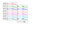
Figure 2: (Color Online) Conventions used in all the figures for the labeling of individual states and of the chemical potential.

As discussed in Sec. II.2, the abnormal extension of the one-body neutron density is usually characterized through the evolution of the neutron r.m.s. radius as one approaches the drip-line, as presented in Fig. 3. A significant kink in the neutron r.m.s. radius is seen at the $N=50$ shell closure. Such a kink is usually interpreted as a signature of the emergence of a neutron halo Meng and Ring (1998); Mizutori et al. (2000). However, this could equally be due to a simple shell effect. Indeed, as the $N=50$ gap is crossed, the two-neutron separation energy $S_{2n}$ drops, as seen in Fig. 4. As a result, the decay constant $\kappa_{0}$ of the one-body density is largely reduced. However, a genuine halo phenomenon relates more specifically to the presence of nucleons which are spatially decorrelated from a core. Even though the case of drip-line Cr isotopes seems favorable, as the $S_{2n}$ drops to almost zero at $N=50$, the occurrence of a halo cannot be thoroughly addressed by only looking at the evolution of the neutron r.m.s. radius.

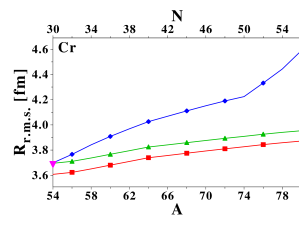
Figure 3: (Color Online) Same as Fig. 1 for proton ($\blacksquare$), neutron ($\blacklozenge$) and charge ($\blacktriangle$) r.m.s. radii. Experimental values for charge r.m.s. radii are indicated when available ($\blacktriangledown$), along with experimental error bars Angeli (2004).

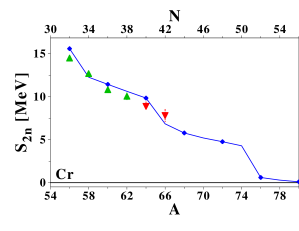
Figure 4: (Color Online) Same as Fig. 1 for two-neutron separation energies $S_{2n}$ ($\blacklozenge$). Experimental values are indicated when available Audi et al. (2003) ($\blacktriangle$ when both masses are known, $\blacktriangledown$ when at least one comes from mass extrapolation), along with experimental error bars.

III.1.2 Tin isotopes

Sn isotopes ($Z=50$) are considered as a milestone for EDF methods and are rather easy to produce in radioactive beam experiments because of their magic proton number. In particular, the fact that it is a long isotopic chain is convenient for systematic studies. At the neutron drip-line, which corresponds to ¹⁷⁴Sn for the {SLy4+REG-M} parameter set, the least-bound orbitals are mostly odd-parity states. Among them, $3p_{3/2}$ and $3p_{1/2}$ states might contribute significantly to the formation of a halo (Fig. 5).

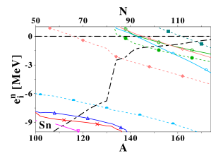
Figure 5: (Color Online) Same as Fig. 1 for Sn isotopes.

However, whereas those $\ell=1$ states are relatively well bound, the least bound orbital is the $1i_{13/2}$ ($\ell=6$) intruder state which is strongly affected by the confining centrifugal barrier. Nevertheless, the neutron r.m.s. radius (Fig. 6) exhibits a weak kink at the $N=82$ shell closure, which has been interpreted as a halo signature Mizutori et al. (2000).

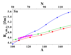
Figure 6: (Color Online) Same as Fig. 3 for Sn isotopes.

As pointed out previously, an analysis based only on r.m.s. radii is incomplete and can even be misleading. Indeed, although the shell effect at the $N=82$ magic number generates a sudden decrease of the $S_{2n}$, the latter does not drop to zero, as seen in Fig. 7. A direct connection between the kink of the r.m.s. radius and the formation of a neutron halo is thus dubious. This point will be further discussed below.

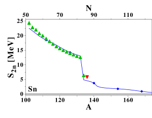
Figure 7: (Color Online) Same as Fig. 4 for Sn isotopes.

In any case, the analysis based on neutron r.m.s. radii is useful but insufficient to characterize halo in a manner that allows the extraction of information useful to nuclear structure and theoretical models. The characterization of halos through the definition of the neutron matter thickness and the one-neutron region thickness is possible Im and Meng (2000) but remains arbitrary and correlated to a one-neutron halo hypothesis. Another way is to extract so-called ”halo factors” from the individual spectrum through antiproton annihilation probing the nuclear density extension Lubiński et al. (1998); Nerlo-Pomorska et al. (2000). However, such tools do not allow the extraction of quantitative properties, such as the actual number of nucleons participating in the halo. They also define the halo as the region where the neutron density dominates the proton one, which is an admixture of the neutron skin and the (potential) halo.

III.2 The Helm model

III.2.1 Introduction

The Helm model has recently been exploited to remedy to the lack of quantitative measure of halo existence and properties Mizutori et al. (2000). Originally, the purpose of the Helm model Refs. Helm (1956); Rosen et al. (1957); Raphael and Rosen (1970) was to fit experimental charge densities, using a few-parameter anzatz, in view of analyzing electron scattering data. The normalized nuclear charge density is approximated by the convolution of a sharp-sphere density of radius $R_{0}$ defining the nuclear extension and of a gaussian of width $\sigma$ describing the surface thickness. The r.m.s. radius of the Helm density solely depends on $R_{0}$ and $\sigma$ and reads as

$$R_{\mathrm{r.m.s.}}^{H}=\sqrt{\frac{\int\rho_{H}(r)\,r^{4}\,dr}{\int\rho_{H}(r)\,r^{2}\,dr}}=\sqrt{\frac{3}{5}\left(R_{0}^{2}+5\sigma^{2}\right)}\,.$$ (13)

This model has been used to study neutron skins and halos in medium-mass nuclei close to the neutron drip-line Mizutori et al. (2000). Proton and neutron densities were defined as a superposition of a core density $\rho^{q}_{\mathrm{core}}$ plus a tail density $\rho^{q}_{\mathrm{tail}}$ describing, when appropriate, the halo. The idea was to reproduce the core part $\rho^{q}_{\mathrm{core}}$ using the Helm anzatz $\rho^{q}_{H}$, normalized to the nucleon number $N^{q}$ ($N^{q}=N$ or $Z$). Thus, the two free parameters $(R_{0}^{q},\sigma^{q})$ were adjusted on the high momentum part of the realistic form factor

$$F^{q}(k)=4\pi\int\rho^{q}(r)\,r^{2}\,j_{0}(k\,r)\,dr\,,$$ (14)

where $\rho^{q}(r)$ is the density coming out of the many-body calculations. It was suggested in Ref. Mizutori et al. (2000) to evaluate (i) $R^{q}_{0}$ through the first zero $k_{1}^{q}$ of the realistic form factor: $R^{q}_{0}=z_{1}^{1}/k_{1}^{q}$, where $z_{1}^{1}$ is the first zero of the Bessel function $j_{1}$ ($z_{1}^{1}\approx 4.49341$), and (ii) $\sigma^{q}$ by comparing the model and realistic form factors at their first extremum $k^{q}_{M}$ (a minimum in the present case). Then, the following radii are defined (i) $R_{\mathrm{geom}}(q)=\sqrt{5/3}\,R_{\mathrm{r.m.s.}}(q)$ (geometric radius) for realistic densities, and (ii) $R_{\mathrm{Helm}}(q)=\sqrt{5/3}\,R_{\mathrm{r.m.s.}}^{H}(q)=\sqrt{{R^{q}_{0}}^{2}+5\,{\sigma^{q}}^{2}}$ (Helm radius) for model densities.

Adjusting the Helm parameters to the high momentum part of the realistic form factor was meant to make the fitting procedure as independent of the asymptotic tail of $\rho^{q}(r)$ as possible. Constructed in this way, $R_{\mathrm{Helm}}(n)$ should not incorporate the growth of $R_{\mathrm{geom}}(n)$ when the neutron separation energy drops to zero and the spatial extension of weakly-bound neutrons increases dramatically. In addition, it was checked that the difference between $R_{\mathrm{Helm}}(p)$ and $R_{\mathrm{geom}}(p)$ was negligible near the neutron drip-line. From these observations, the neutron skin and neutron halo contributions to the geometric radius were defined as⁽⁾

$$\left\{\begin{array}[]{l}\displaystyle\Delta R_{\mathrm{skin}}\equiv R_{\mathrm{Helm}}(n)-R_{\mathrm{Helm}}(p)\,\,\,,\\ \\ \displaystyle\Delta R_{\mathrm{halo}}\equiv R_{\mathrm{geom}}(n)-R_{\mathrm{Helm}}(n)\,\,\,.\end{array}\right.$$ (15)

III.2.2 Limitations of the Helm model

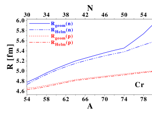
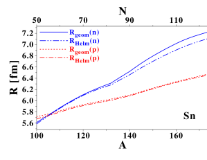
Figure 8: (Color Online) Geometric and Helm radii for Cr and Sn isotopes calculated in the spherical HFB approach with the {SLy4+REG-M} functional.

Proton and neutron Helm radii are compared to geometric ones on Fig. 8 for chromium and tin isotopes. The behavior of $R_{\mathrm{geom}}(q)$ and $R_{\mathrm{Helm}}(q)$ for Sn isotopes is the same as in Ref. Mizutori et al. (2000)⁽⁾. For both isotopic chains, the sudden increase of the neutron geometric radius beyond the last neutron shell closure might be interpreted as a signature of a halo formation. However, $\Delta R_{\mathrm{halo}}$ is non-zero along the entire Cr isotopic chain, even on the proton-rich side. The latter result is problematic as neutron halos can only be expected to exist at the neutron drip-line.

Such non-zero values for $\Delta R_{\mathrm{halo}}$ can be understood as a direct consequence of the gaussian folding in the definition of the Helm density. The asymptotic decay of the Helm density is roughly quadratic in logarithmic scale, instead of being linear Dobaczewski et al. (1984, 1996); Tajima (2004). To illustrate this point, Fig. 9 displays the realistic and Helm densities of ⁵⁴Cr (in the valley of stability) and ⁸⁰Cr (drip-line nucleus). The difference in the asymptotic behaviors is obvious. In particular, the Helm densities are unable to reproduce the correct long-range part of the non-halo proton density, or the neutron density of nuclei in the valley of stability.

Such features lead to unsafe predictions for the halo parameter $\Delta R_{\mathrm{halo}}$ as the neutron skin and the potential halo are not properly separated. Such problems, as well as a lack of flexibility to account for finer details of the nuclear density had already been pointed out Friedrich and Voegler (1982).

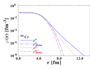
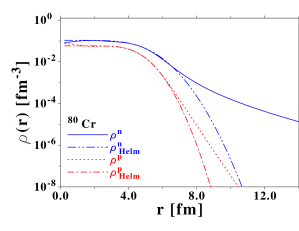
Figure 9: (Color Online) Realistic and Helm densities of ⁵⁴Cr and ⁸⁰Cr.

One might thus question the fitting procedure introduced in Ref. Mizutori et al. (2000). The method naturally requires $R^{q}_{0}$ and $\sigma^{q}$ to be adjusted on the form factor at sufficiently large $k$ so that the Helm density relates to the core part of the density only. Of course, some flexibility remains, e.g. one could use the second zero $k_{2}^{q}$ of $F^{q}(k)$ to adjust $R_{0}^{q}$. Following such arguments, four slightly different adjustment procedures $A_{i}$, $i=1,4$, all consistent with the general requirement exposed above, have been tested to check the stability of the Helm model

$A_{1}$

: (i) $F^{q}_{H}(k^{q}_{1})=F(k^{q}_{1})$ (ii) $F^{q}_{H}(k^{q}_{M})=F^{q}(k^{q}_{M})$ ,

$A_{2}$

: (i) $F^{q}_{H}(k^{q}_{1})=F^{q}(k^{q}_{1})$ (ii) ${F^{q}_{H}}^{\prime}(k^{q}_{1})={F^{q}}^{\prime}(k^{q}_{1})$ ,

$A_{3}$

: (i) $F^{q}_{H}(k^{q}_{2})=F^{q}(k^{q}_{2})$ (ii) ${F^{q}_{H}}^{\prime}(k^{q}_{2})={F^{q}}^{\prime}(k^{q}_{2})$ ,

$A_{4}$

: (i) $F^{q}_{H}(k^{q}_{1})=F^{q}(k^{q}_{1})$ (ii) ${F^{q}_{H}}^{\prime}(0.4\,k^{q}_{1})={F^{q}}^{\prime}(0.4\,k^{q}_{1})$ .

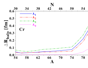
Figure 10: (Color Online) Halo parameter $\Delta R_{\mathrm{halo}}$ for chromium isotopes using different fitting procedures for the Helm parameters $(R_{0}^{q},\sigma^{q})$ (see text).

Fig. 10 shows the halo parameter $\Delta R_{\mathrm{halo}}$ obtained for Cr isotopes using protocols $A_{1}$ to $A_{4}$. Note that protocol $A_{1}$ is the one proposed in Ref. Mizutori et al. (2000) and used earlier whereas the weight of the long distance part of the realistic density is more important in protocol $A_{4}$. Although the general pattern remains unchanged, the halo parameter significantly depends on the fitting procedure used to determine $(R^{q}_{0},\sigma^{q})$. Because of the wrong asymptotic behavior of the Helm density discussed above, one cannot make $\Delta R_{\mathrm{halo}}$ to be zero for magic and proton-rich nuclei (see protocol $A_{4}$), keeping unchanged its values for halo candidates at the neutron drip-line⁽⁾. Such a fine tuning of the fitting procedure that would make use of an a priori knowledge of non-halo nuclei is impractical and unsatisfactory.

As a next step, we tried to use other trial densities to improve on the standard Helm model. A key feature is to obtain an analytical expression of the associated model form factor in order to adjust easily its free parameters. We could not find any form leading to both an analytical expression of $F^{q}_{H}$ and good asymptotic, with only two free parameters⁽⁾.

Although the Helm model looked promising at first, we have shown the versatility of its predictions. The inability of the model to describe the correct asymptotic of the nuclear density in the valley of stability, as well as the too large freedom in the fitting procedure, limit very much its predictive power. Therefore a more robust analysis method is needed to characterize medium-mass halo nuclei.

IV New criterion for a quantitative analysis of halo systems

Although deceiving, the previous attempts have underlined the following point: a useful method to study halos must be able to characterize a spatially decorrelated component in the nucleon density in a model-independent fashion. We propose in the following a method which allows the identification of such a contribution to the internal one-body density. Our starting point is a thorough analysis of medium-range and large-distance properties of the one-body internal density in Sec. IV.1. Based on such an analysis, new quantitative criteria to identify and characterize halos are defined in Sec. IV.2. We already outline at this point that the analysis and the associated criteria are applicable to any finite many-fermion system, as long as the inter-fermion interaction is negligible beyond a certain relative distance. As done throughout the article, atomic nuclei are used as typical examples in the present section.

IV.1 Properties of the one-body density

IV.1.1 Definitions and notations

Let us start from the non-relativistic $N$-body Hamiltonian⁽⁾

$${H}^{N}\equiv\sum_{i=1}^{N}\frac{p_{i}^{2}}{2m}+\sum_{\begin{subarray}{c}i,j=1\\ i<j\end{subarray}}^{N}V(r_{ij})\,\,,$$ (16)

where $p_{i}$ is the single-particle momentum, $r_{ij}\equiv|\vec{r}_{i}-\vec{r}_{j}\,|$ and $V$ denotes the vacuum nucleon-nucleon interaction. The nuclear Hamiltonian ${H}^{N}$ is invariant under translation and can be written as a sum of a center-of-mass part ${H}^{N}_{\mathrm{c.m.}}$ and an internal part ${H}^{N}_{\mathrm{int}}$. Thus, eigenstates of ${H}^{N}$, denoted by ${\Psi}^{N}_{i,\vec{K}}(\vec{r}_{1}\ldots\vec{r}_{N})$, can be factorized into the center-of-mass part (plane wave) times the internal wave function

$${\Psi}^{N}_{i,\vec{K}}(\vec{r}_{1}\ldots\vec{r}_{N})=e^{i\,\vec{K}\cdot\vec{R}_{N}}\,\Phi^{N}_{i}(\vec{\xi}_{1}\ldots\vec{\xi}_{N-1})\,\,\,,$$ (17)

where $\vec{K}$ is the total momentum and $\vec{R}_{N}$ the center-of-mass position

$$\vec{R}_{N}\equiv\frac{1}{N}\sum_{i=1}^{N}\vec{r}_{i}\,.$$ (18)

The word internal relates to the fact that the wave function $\Phi^{N}_{i}$ can be expressed in terms of relative coordinates only, such as the $(N-1)$ independent Jacobi variables

$$\vec{\xi}_{i}\equiv\vec{r}_{i+1}-\frac{1}{i}\sum_{j=1}^{i}\vec{r}_{j}\,,$$ (19)

and is associated with the internal energy $E_{i}^{N}$. A consequence is that $\Phi^{N}_{i}$ is invariant under translation of the system in the laboratory frame.

The ground-state internal wave function $\Phi_{0}^{N}$ can be expanded in terms of the complete orthonormal set of internal $(N-1)$-body wave functions $\{\Phi^{N-1}_{\nu}\}$, which are eigenstates of the $(N-1)$-body internal Hamiltonian Van Neck et al. (1996, 1998); Van Neck and Waroquier (1998); Escher et al. (2001)

$${H}^{N-1}_{\mathrm{int}}\,{\Phi}^{N-1}_{\nu}(\vec{r}_{1}\ldots\vec{r}_{N-1})={E}^{N-1}_{\nu}\,{\Phi}^{N-1}_{\nu}(\vec{r}_{1}\ldots\vec{r}_{N-1})\,,$$ (20)

such that

$$\Phi_{0}^{N}(\vec{r}_{1}\ldots\vec{r}_{N})=\frac{1}{\sqrt{N}}\sum_{\nu}{\Phi^{N-1}_{\nu}}(\vec{r}_{1}\ldots\vec{r}_{N-1})\\ \times\varphi_{\nu}(\vec{r}_{N}-\vec{R}_{N-1})\,.$$ (21)

The states $\Phi^{N-1}_{\nu}$ are ordered by increasing energies, $\nu=0$ corresponding to the ground state of the $(N-1)$-body system. The norm of the overlap functions $\varphi_{\nu}(\vec{r}\,)$ provides the so-called spectroscopic factors Clément (1973a, b)

$$S_{\nu}=\int d\vec{r}\,|\varphi_{\nu}(\vec{r}\,)|^{2}\,.$$ (22)

Finally, the relevant object to be defined for self-bound systems is the internal one-body density matrix Van Neck et al. (1993); Van Neck and Waroquier (1998); Shebeko et al. (2006)

$$\rho_{\mathrm{[1]}}(\vec{r},\vec{r}\,^{\prime}) \equiv \sum_{\nu}\varphi^{*}_{\nu}(\vec{r}\,^{\prime})\varphi_{\nu}(\vec{r}\,)\,,$$ (23)

which is completely determined by the overlap functions Van Neck et al. (1993). The actual internal one-body density $\rho_{\mathrm{[1]}}(\vec{r}\,)=\rho_{\mathrm{[1]}}(r)$ is extracted as the local part of the internal density matrix

$$\rho_{\mathrm{[1]}}(r)\equiv\sum_{\nu}|\varphi_{\nu}(\vec{r}\,)|^{2}=\sum_{\nu}\frac{2\ell_{\nu}+1}{4\pi}|\bar{\varphi}_{\nu}(r)|^{2}\,,$$ (24)

where the energy degeneracy associated with the orbital momentum has been resolved through the summation over the spherical harmonics.

IV.1.2 Long-distance behavior and ordering of the $\varphi_{\nu}(\vec{r}\,)$

For large distance, i.e. $r>R$, the nuclear interaction vanishes and the asymptotic radial part $\bar{\varphi}_{\nu}$⁽⁾ of the overlap function is solution of the free Schrödinger equation with a reduced mass $m_{\mathrm{red}}=m(N-1)/N$

$$\left[\left(\frac{d^{2}}{dr^{2}}+\frac{2}{r}\frac{d}{dr}-\frac{\ell_{\nu}(\ell_{\nu}+1)}{r^{2}}\right)-\kappa_{\nu}^{2}\right]\bar{\varphi}_{\nu}^{\infty}(r)=0\,,$$ (25)

with $\kappa_{\nu}=\sqrt{-2m_{\mathrm{red}}\epsilon_{\nu}/\hbar^{2}}$, and $\epsilon_{\nu}=\left(E_{0}^{N}-E_{\nu}^{N-1}\right)$ is minus the one-nucleon separation energy to reach $\Phi_{\nu}^{N-1}$. Solutions of the free Shrödinger equation take the form

$$\varphi_{\nu}^{\infty}(\vec{r}\,)=B_{\nu}\,h_{\ell_{\nu}}(i\,\kappa_{\nu}\,r)\,Y_{\ell_{\nu}}^{m_{\nu}}(\theta,\varphi)\,.$$ (26)

As a result, the internal one-body density behaves at long distances as⁽⁾

$$\rho_{\mathrm{[1]}}^{\infty}(r)=\sum_{\nu}\frac{B_{\nu}^{2}}{4\pi}(2\ell_{\nu}+1)|h_{\ell_{\nu}}(i\,\kappa_{\nu}r)|^{2}\,\,.$$ (27)

For very large arguments, the squared modulus of a Hankel function behaves as $e^{-2\kappa_{i}r}/(\kappa_{i}r)^{2}$ Abramowitz and Stegun (1965). Thus the $\nu=0$ component dominates and provides the usual asymptotic behavior Dobaczewski et al. (1984, 1996); Tajima (2004)⁽⁾

$$\rho_{\mathrm{[1]}}^{\infty}(r)\underset{r\rightarrow+\infty}{\longrightarrow}\frac{B_{0}^{2}}{4\pi}(2\ell_{0}+1)\frac{e^{-2\kappa_{0}\,r}}{(\kappa_{0}\,r)^{2}}\,.$$ (28)

The asymptotic form of the Hankel function is independent of the angular momentum which explains why high-order moments $\langle r^{n}\rangle$ of the density diverge when high-$\ell$ states are loosely bound, as discussed in Sec. II.2. Thus, the contributions of the overlap functions to $\rho_{\mathrm{[1]}}^{\infty}$ at very large distances are ordered according to their associated separation energies $|\epsilon_{\nu}|$, independently of $\ell_{\nu}$. Corrections to this ordering at smaller distances come from (i) the $\ell$-dependence of the Hankel functions due to the centrifugal barrier, which favors low angular momentum states, and (ii) the $(2\ell+1)$ degeneracy factor which favors high angular momentum states. In any case, for extremely large distances the least bound component will always prevail, although this may happen beyond simulation reach.

To characterize the net effect of corrections (i) and (ii) on the relative positioning of overlap functions at long distances, the contributions $(2\ell_{\nu}+1)|\bar{\varphi}_{\nu}(r)|^{2}$, for a fixed energy but different angular momenta, are compared in Fig. 11 for the solutions of a simple finite spherical well. Outside the well, Hankel functions are exact solutions of the problem. The potential depth is adjusted to obtain identical eigenenergies for all $\ell_{\nu}$. Although the $(2\ell_{\nu}+1)$ factor reduces the gap between $s$ and $p$ components, the effect of the centrifugal barrier is always the strongest at large $r$, where states are clearly ordered according to $\ell_{\nu}$, favoring low angular momenta. In any case, the separation energy remains the leading factor as far as the ordering of overlap functions at long distances is concerned.

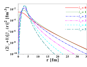
Figure 11: (Color Online) Squared components of the solutions of a finite spherical well of fixed radius $a=4$ fm, multiplied by the degeneracy factor $(2\ell_{\nu}+1)$, for various angular momenta and fixed energy $\epsilon_{\nu}=-100$ keV. The first state for each $\ell_{\nu}$ (nodeless component corresponding to a primary quantum number equal to zero) is represented.

IV.1.3 Crossing pattern in $\rho_{\mathrm{[1]}}^{\infty}(r)$

The (model-independent) ordering at long distances of individual components entering $\rho_{\mathrm{[1]}}^{\infty}$ has interesting consequences on the properties of the density as a whole. As discussed below, this ordering induces a typical crossing pattern between the individual components which will eventually be used to characterize halo nuclei.

Introducing normalized overlap functions $\psi_{\nu}(\vec{r}\,)$, Eq. (24) becomes

$$\rho_{\mathrm{[1]}}(r)=\sum_{\nu}\frac{2\ell_{\nu}+1}{4\pi}\,S_{\nu}\,\left|\bar{\psi}_{\nu}(r)\right|^{2}\equiv\sum_{\nu}C_{\nu}(r)\,.$$ (29)

Let us take all spectroscopic factors equal to one for now. The $\nu=0$ component, corresponding to the smallest separation energy, dominates at large distances. Because of continuity and normalization conditions, this implies that $\bar{\psi}_{0}(r)$ has to cross all the other overlap functions as $r$ goes inward from $+\infty$ to zero. The position at which $\psi_{0}$ crosses each $\psi_{\nu}$ depends on the difference of their separation energies and on their angular momenta. In particular, there will exist a crossing between $|\bar{\psi}_{0}(r)|^{2}$ and the remaining density $\left[\rho^{[1]}(r)-C_{0}(r)\right]$. The same is true about $|\bar{\psi}_{1}(r)|^{2}$: it must cross the remaining density $\left[\rho^{[1]}(r)-C_{0}(r)-C_{1}(r)\right]$… As a result, any given individual component must cross the sum of those that are more bound. Of course, the centrifugal barrier influences the position of such crossings but not their occurrence because of the robustness of the (very) asymptotic ordering pattern discussed in the previous section.

Let us now incorporate the role of spectroscopic factors. In practice, $S_{\nu}$ is known to increase with the excitation energy of the corresponding eigenstate of the $(N-1)$-body system. Thus, the norm of $\varphi_{0}$ is smaller than those of the excited components $\varphi_{\nu}$, which mechanically ensures the existence of the crossings discussed previously. A similar reasoning holds when going from $\varphi_{0}$ to $\varphi_{1}$ etc.

One should finally pay attention to the number of nodes of the overlap function $\bar{\varphi}_{\nu}$. This feature actually favors low angular momentum states as far as the asymptotic positioning is concerned. If two components have the same energy but different angular momenta, the one with the lowest $\ell$ will have a greater number of nodes. This will reduce the amplitude of the wave function in the nuclear interior. That is, the weight of the asymptotic tail is increased, which favors its dominance at long distance. However, this effect is expected to have a small impact in comparison with the other corrections discussed above. As a result, the crossing pattern between the components of the density is not jeopardized by the existence of nodes in the overlap functions.

IV.2 Halo characterization

IV.2.1 Definition

The discussion of Sec. IV.1.3 demonstrates how individual contributions to the one-body density (i) are positioned with respect to each other (ii) display a typical crossing pattern. Such features are now used to characterize halo systems.

As pointed out earlier, one general and model-independent definition of a halo relates to the existence of nucleons which are spatially decorrelated from others, constituting the core. This can only be achieved if some contributions to the internal density exhibit very long tails. Most importantly, the delocalization from the core requires the latter to exist and to remain well localized. To achieve such a spatial decorrelation between a core and a tail part, it is necessary to have a crossing between two well-identified groups of orbitals with significantly different asymptotic slopes. This translates into a sharp crossing between those two groups of orbitals and thus to a pronounced curvature in the density. Note that this explains the empirical observation that the first logarithmic derivative of the density invariably displays a minimum at some radius Stoitsov et al. (2003). How much this feature is pronounced or not is key and will be used in the following to design model-independent criteria to characterize halo systems.

A pronounced crossing is illustrated in Fig. 12 for a simple model where the halo is due to a single orbital. Of course, more complex situations have to be considered where multiple states contribute to the core and the halo. Indeed, the presence of collective motions in medium-mass systems implies that one hardly expects a single orbital to be well separated from the others.

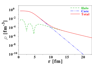
Figure 12: (Color Online) ”Core+tail” simplified model. The total density is the superposition of a well-bound component and a loosely-bound one. A semi-phenomenological density (see Appendix B) is used for the core density, whereas the halo part is the realistic $3_{1/2}$ state of ⁸⁰Cr obtained from spherical HFB calculations with the {SLy4+REG-M} functional.

IV.2.2 Relevant energy scales

The need for the existence of two groups of orbitals characterized by significantly different asymptotic slopes provides critical conditions for the appearance of a halo: (i) the least bound component $\varphi_{0}$ must have a very small separation energy to extend far out, (ii) several components $\varphi_{1},\varphi_{2}\ldots\varphi_{m}$ may contribute significantly to the density tail if, and only if, they all have separation energies of the same order as that of $\varphi_{0}$, (iii) for this tail to be spatially decorrelated from the rest of the density (the ”core”), the components with $\nu>\nu_{m}$ have to be much more localized than those with $\nu\leq\nu_{m}$. This third condition is fulfilled when the crossing between the $m^{th}$ and $(m+1)^{th}$ components in the density is sharp, which corresponds to significantly different decay constants $\kappa_{m}\ll\kappa_{m+1}$ at the crossing point.

The later situation translates eventually into specific patterns in the excitation energy spectrum of the $(N-1)$-body system. It suggests that a halo appears when (i) the one-neutron separation energy $S_{n}=|\epsilon_{0}|$ is close to zero, (ii) a bunch of low energy states in the $(N-1)$-body system have separation energies $|\epsilon_{\nu}|$ close to zero, and (iii) a significant gap in the spectrum of the $(N-1)$-body system exists, which separates the latter bunch of states $\varphi_{\nu}$ from higher excitations.

A similar discussion was given in the context of designing an effective field theory (EFT) for weakly-bound nuclei Bertulani et al. (2002), where two energy scales $(E,E^{\prime})$ were found to be relevant: (i) the nucleon separation energy $E=S_{n}$ which drives the asymptotic behavior of the one-body density, and (ii) the core excitation energy $E^{\prime}=|\epsilon_{m+1}|$ which needs to be such as $E^{\prime}\gg E$, in order for the tail orbitals to be well decorrelated from the remaining core. The additional energy scale that we presently identify is the energy spread $\Delta E$ of the low-lying states in the $(N-1)$-body system, which becomes relevant when more than one component is involved in the halo. The corresponding picture is displayed in the bottom panel of Fig. 13 and is also translated in terms of canonical energies $e_{i}$ in the upper panel of the same figure.

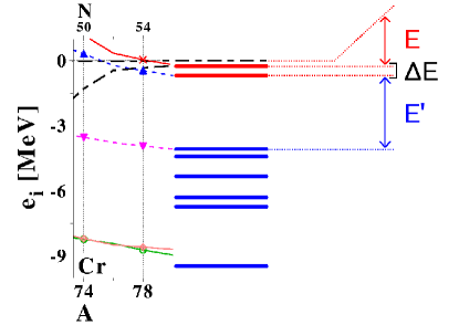
(a)  Canonical neutron energy spectrum $e_{i}$.

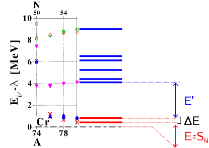
(b)  Separation energy spectrum $|\epsilon_{\nu}|$ for the $(N-1)$-body system.

Figure 13: (Color Online) Schematic display of the energy scales relevant for the appearance of halos (right-hand side). The realistic spectra obtained through HFB calculations of the four last bound chromium isotopes are shown on the left-hand sides.

More quantitatively, the ideal situation for the formation of a halo is obtained for (i) a very small separation energy, in orders of a few hundred keVs, the empirical value of $2$ MeV$/A^{2/3}$ from Refs. Fedorov et al. (1993); Jensen and Riisager (2000) giving a good approximation of expected values, (ii) a narrow bunch of low-lying states, whose spread $\Delta E$ should not exceed about one MeV, and (iii) a large gap $E^{\prime}$ with the remaining states, at least four or five times the separation energy $E$. Those are only indicative values, knowing that there is no sharp limit between halo and non-halo domains.

IV.2.3 Halo region

As discussed in the previous section, a halo can be identified through a pronounced ankle in the density, due to the sharp crossing between the aggregated low-lying components and the upper-lying ones. Such a large curvature translates into a peak in the second derivative of the (base-$10$) logarithmic profile ($\log_{10}$) of the one-body density, as seen in Fig. 14 for a schematic calculation.

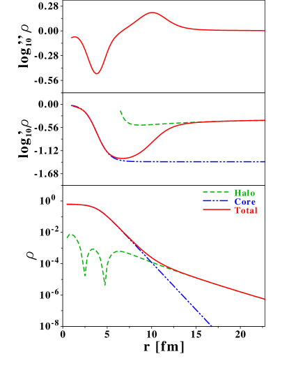
Figure 14: (Color Online) Ankle in the (base-$10$) log-density due to the presence of a low-lying state well separated from the remaining ones: log-density (bottom panel), first (middle panel) and second (top panel) log-derivatives. The conventions are the same as in Fig. 12.

At the radius $r=r_{max}$ corresponding to the maximum of that peak, core and tail contributions cross; i.e. they contribute equally to the total density. At larger radii, the halo, if it exists, dominates. Therefore, we define the spatially decorrelated region as the region beyond the radius $r_{0}$ where the core density is one order of magnitude smaller than the halo one. In practice, the previous definition poses two problems. First, in realistic calculations, one only accesses the total density. Second, the choice of one order of magnitude is somewhat arbitrary.

Extensive simulations have been performed to characterize $r_{0}$ unambiguously, using either one or several contributions to the halo density, and covering large energy ranges for $E$, $E^{\prime}$ and $\Delta E$. More details on the method used to find the best approximation to $r_{0}$, as well as the corresponding theoretical uncertainty, are given in Appendix B. Given $r_{max}$, which can be extracted from the total density, it has been found that $r_{0}$ can be reliably defined through

$$\left\{\begin{array}[]{l}r_{0}>r_{max}\,,\\ \\ \displaystyle\frac{\partial^{2}\log_{10}{\rho(r)}}{\partial r^{2}}\biggl{|}_{\displaystyle r=r_{0}}\equiv\frac{2}{5}\,\frac{\partial^{2}\log_{10}{\rho(r)}}{\partial r^{2}}\biggl{|}_{\displaystyle r=r_{max}}\,,\end{array}\right.$$ (30)

as exemplified in Fig. 15. Also, theoretical uncertainties on the determination of $r_{0}$ are introduced, such that

$$0.35\leq\frac{\log_{10}^{\prime\prime}(\rho(r_{0}))}{\log_{10}^{\prime\prime}(\rho(r_{max}))}\leq 0.50\,,$$ (31)

where ^′ denotes a compact notation for $\partial/\partial r$.

Once validated by simulations, the method to isolate the halo region only relies on the density as an input, and does not require an a priori separation of the one-body density into core and halo parts. Finally, one may note that our definition of the halo region does not a priori exclude contributions from individual components with angular momenta greater than one.

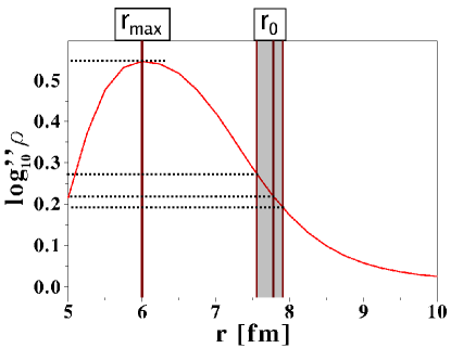
Figure 15: (Color Online) Definition of $r_{0}$ through the second derivative of the log-density, using the same model density as in Fig. 14. $r_{0}$ is represented by the central vertical line. The shaded area corresponds to the tolerance margin on $r_{0}$ (see text).

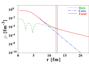
Figure 16: (Color Online) Consequences of the definition of $r_{0}$ (vertical lines for the values of $r_{0}$ and the tolerance margin - see text) in the same model as in Fig. 14. The halo density dominates the core part by around one order of magnitude.

IV.2.4 Halo criteria

We now introduce several criteria to characterize the halo in a quantitative way, by applying the previous analysis to the neutron one-body density⁽⁾. First, the average number of nucleons in the halo region can be extracted through

$$N_{\mathrm{halo}}\equiv 4\pi\int_{r_{0}}^{+\infty}\!\!\rho^{n}(r)\,r^{2}\,dr\,\,\,.$$ (32)

An important information is the effect of the halo region on the radial moments of the density. By definition, the contribution of the core to any moment $\langle r^{n}\rangle$ is negligible for $r\geq r_{0}$. It has been checked in the case of the r.m.s. radius, and is all the more true as $n$ increases. Thus, one can evaluate the effect of the decorrelated region on the nuclear extension through

$$\delta R_{\mathrm{halo}} \equiv R^{n}_{\mathrm{r.m.s.},tot}-R^{n}_{\mathrm{r.m.s.},inner}$$ (33)

$$= \!\!\!\!\sqrt{\frac{\int_{0}^{+\infty}\rho^{n}(r)r^{4}\,dr}{\int_{0}^{+\infty}\rho^{n}(r)r^{2}\,dr}}-\sqrt{\frac{\int_{0}^{r_{0}}\rho^{n}(r)r^{4}\,dr}{\int_{0}^{r_{0}}\rho^{n}(r)r^{2}\,dr}}\,.$$

The quantity $\delta R_{\mathrm{halo}}$ is similar to $\Delta R_{\mathrm{halo}}$ defined within the Helm model (Eq. (15)). However, the former does not rely on any a priori decomposition of the density into core and halo components. That is of critical importance. Extensions to all radial moments of the density can be envisioned⁽⁾.

The quantities $N_{\mathrm{halo}}$ and $\delta R_{\mathrm{halo}}$ are of course correlated, but they do not carry exactly the same information. Note that tolerance margins on $r_{0}$ from Eq. (31) propagate into theoretical uncertainties on $N_{\mathrm{halo}}$ and $\delta R_{\mathrm{halo}}$.

In the case of stable/non-halo nuclei, both quantities will be extremely small. There is still a slight curvature in the density profile that provides a radius $r_{0}$ but the computed criteria will be consistent with zero. In the particular case of magic neutron number, the curvature becomes particularly weak and translates into a broad peak in the second log-derivative. As a result, the radius $r_{0}$ value is large and defines a region where the density is particularly low. This is illustrated by Fig. 17, where $r_{0}$ is plotted for chromium isotopes as a function of $A$. The maximum of $r_{0}$ is attained for the magic shell $N=50$.

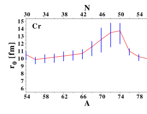
Figure 17: (Color Online) Evolution of $r_{0}$ along the Cr isotopic chain, obtained through spherical HFB calculations with the {SLy4+REG-M} functional.

Finally, further characterization of the halo can be achieved by looking at the individual contributions of each overlap function

$$N_{\mathrm{halo},\nu}\equiv 4\pi\,(2j^{n}_{\nu}+1)\,\int_{r_{0}}^{+\infty}|\bar{\varphi}^{n}_{\nu}(r)|^{2}\,r^{2}\,dr\,.$$ (34)

$N_{\mathrm{halo},\nu}$ provides a decomposition of the halo in terms of single-particle-like states. Note that the inner part of an overlap function, i.e. for $r<r_{0}$, does not contribute to halo observables.

By analogy with the criterion used for light halo systems, the probability of each individual overlap function $\varphi_{\nu}$ to be in the $r\geq r_{0}$ region can be defined through

$$P_{\nu}\equiv\frac{\displaystyle\int_{r_{0}}^{+\infty}|\bar{\varphi}_{\nu}(r)|^{2}\,r^{2}\,dr}{\displaystyle\int_{0}^{+\infty}|\bar{\varphi}_{\nu}(r)|^{2}\,r^{2}\,dr}\,.$$ (35)

V Application to EDF calculations

We apply the analysis method introduced in Sec. IV to results obtained from self-consistent HFB calculations of chromium and tin isotopes. In Sec. IV, the energies $\epsilon^{q}_{\nu}$ that characterize internal overlap functions denote exact nucleon separation energies. No approximation to the nuclear many-body problem was involved in the analysis conducted in Sec. IV. The patterns of the internal one-body density thus extracted are fully general and model-independent.

In practice of course, one uses an approximate treatment of the quantum many-body problem. This raises critical questions in the case of EDF calculations as discussed in Appendix A.2. Indeed, the one-body density at play in single-reference EDF calculations is an intrinsic density rather than the internal density, i.e. it is the laboratory density computed from a symmetry breaking state. As is customary in EDF methods though, one uses such an intrinsic density to approximate the internal density; e.g. when analyzing electron scattering data. Of course, such an identification is not rigourously justified and formulations of EDF methods directly in terms of the internal density are currently being considered Engel (2007). Still, the asymptotic part of the lower component $V^{q}_{\nu}(\vec{r}\,)$ of the HFB quasiparticle wave-function satisfies the free Schrödinger equation Bennaceur and Dobaczewski (2005) (Eq. 25), just as the true internal overlap function $\varphi_{\nu}(\vec{r}\,)$ does. Considering in addition that the intrinsic HFB one-body density reads as

$$\rho^{q}(r)\equiv\sum_{\nu}\,\frac{2j^{q}_{\nu}+1}{4\pi}\,|\bar{V}^{q}_{\nu}(r)|^{2}\,\,,$$ (36)

one realizes that the analysis performed in Sec. IV, including the existence of the crossing pattern, applies directly to it⁽⁾.

V.1 Implementation of the criteria

In the code HFBRAD, the HFB problem is solved in a spherical box up to a distance $R_{box}$ from the center of the nucleus on a radial mesh of step size $\Delta r=0.25$ fm. For $R_{box}=40$ fm, the mesh has $160$ points in the radial direction, for both the individual wave-functions and the densities. To obtain a satisfactory precision, the second order log-derivative is computed using a five-points difference formula Abramowitz and Stegun (1965). The precision of the formula is the same as the intrinsic precision of the Numerov algorithm used for the integration of second-order differential equations (which is $\mathcal{O}\left(\Delta r^{6}\right)$) Dahlquist and Björck (1974); Bennaceur and Dobaczewski (2005). Approximate positions of the maximum of the second order log-derivative of $\rho^{n}(r)$ and of $r_{0}$ are first determined with a simple comparison algorithm. To increase the precision, a $11$-points polynomial spline approximation to the density and its second log-derivative around the two points of interest is performed. Because the functions involved are regular enough, a spline approximation provides the radii $r_{max}$ and $r_{0}$ with a good precision, as they are obtained using a dichotomy procedure up to a (arbitrary) precision of $10^{-5}$. Finally, the integrations necessary to compute $N_{\mathrm{halo}}$ and $\delta R_{\mathrm{halo}}$ are performed with six-points Gaussian integration.

In the definition of $\delta R_{\mathrm{halo}}$, the core contribution to the total r.m.s. radius is approximated as the root-mean-square radius of the density distribution truncated to its $r<r_{0}$ component. To check the influence of this cut, the core density was extrapolated beyond the point where the second order log-derivative crosses zero⁽⁾ using Eq. (28) and enforcing continuity of $\rho^{n}$ and ${\rho^{n}}^{\prime}$. No difference was seen for $\delta R_{\mathrm{halo}}$.

The individual contributions $N_{\mathrm{halo,i}}$, as well as the individual probabilities $P_{i}$, are evaluated in the canonical basis. Equivalently, $N_{\mathrm{halo},\nu}$ and $P_{\nu}$ can be calculated in the quasiparticle basis. Quasiparticle states are the best approximation to the overlap functions, but canonical and quasiparticle basis really constitute two equivalent pictures. Indeed, each canonical state is, roughly speaking, split into quasiparticle solutions of similar energies. A summation over quasiparticles having the same quantum numbers in an appropriate energy window would recover the single-particle canonical approximation. The latter is preferred here, as it is more intuitive to work in the natural basis.

V.2 Cr isotopes

According to the analysis of Sec. IV.2.2, drip-line chromium isotopes appear to be ideal halo candidates. The separation energy spectrum $|\epsilon^{n}_{\nu}|=E^{n}_{\nu}-\lambda^{n}$ to the states in the $(N-1)$-body system is shown in Fig. 18.

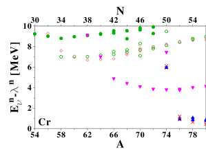
Figure 18: (Color Online) Neutron separation energies $|\epsilon^{n}_{\nu}|=E^{n}_{\nu}-\lambda^{n}$ along the Cr isotopic chain, obtained through spherical HFB calculations with the {SLy4+REG-M} functional. Only relevant quasiparticle energies ($N^{n}_{\nu}>0.01$) are displayed. Conventions for labeling individual states are found in Fig. 2.

Tab. 1 displays the canonical and quasiparticle spectra for the drip-line nucleus ⁸⁰Cr. In the canonical basis, $|e^{n}_{0}|$ is associated with a $3s_{1/2}$ state and is about $180$ keV. The next low-lying state ($2d_{5/2}$) is within an energy interval of $\Delta E\approx 500$ keV. Those two states are separated from a core of orbitals by $E^{\prime}\approx 3.5$ MeV. Equivalently, the separation energy in the quasiparticle basis is $|\epsilon^{n}_{0}|\approx 430$ keV, whereas four quasiparticle states ($s_{1/2}$ and $d_{5/2}$) are with an energy spread of $\Delta E\approx 470$ keV, and are further separated from higher-excited states by $E^{\prime}\approx 3.2$ MeV. The separation energy $S_{n}$ for ⁸⁰Cr is compatible with the phenomenological binding energy necessary for the appearance of light halo nuclei, namely $2$ MeV$/A^{2/3}\approx 137$ keV. According to the discussion of Sec. IV.2.2, the energy scales at play in the three last bound Cr isotopes correspond to ideal halo candidates.

Can. spectrum 80Cr			Exc. spectrum 79Cr
		$e^{n}_{i}$ [MeV]			$E^{n}_{\nu}-\lambda^{n}$ [MeV]
————		$>0$			$>10$
$E\updownarrow$				$f_{5/2}$	8.694
$\Delta E\left\{\vphantom{\begin{array}[]{l}a\\ a\end{array}}\right.$	$3s_{1/2}$	-0.178		$p_{1/2}$	8.960
	$2d_{5/2}$	-0.670		$g_{9/2}$	4.103
$E^{\prime}\left\updownarrow\vphantom{\begin{array}[]{l}a\\ a\\ a\end{array}}\right.$			$E^{\prime}\left\updownarrow\vphantom{\begin{array}[]{l}a\\ a\end{array}}\right.$
			$\Delta E\left\{\vphantom{\begin{array}[]{l}a\\ a\\ a\\ a\end{array}}\right.$	$d_{5/2}$	0.893
	$1g_{9/2}$	-4.062		$d_{5/2}$	0.832
	$1f_{5/2}$	-8.676		$s_{1/2}$	0.728
	$1f_{5/2}$	-8.676		$s_{1/2}$	0.427
	$2p_{1/2}$	-8.942	$E\updownarrow$
		$<-10$	————		$0$

Table 1: (Color Online) Neutron canonical energies $e^{n}_{i}$ in ⁸⁰Cr and separation energies $|\epsilon^{n}_{\nu}|=E^{n}_{\nu}-\lambda^{n}$, as predicted by the {SLy4+REG-M} functional. Quasiparticle states with a spectroscopic factor smaller than $10^{-2}$ are not included.

The criteria introduced in Sec. IV.2.4 are now applied.

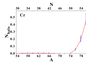
Figure 19: (Color Online) Average number of nucleons participating in the halo along the Cr isotopic chain, as a function of the nuclear mass, as predicted by the {SLy4+REG-M} functional. Theoretical uncertainties are included (see text).

Fig. 19 shows the average number of nucleons participating in the potential halo. Whereas $N_{\mathrm{halo}}$ is consistent with zero for $N\leq 50$, a sudden increase is seen beyond the $N=50$ shell closure. The existence of a decorrelated region in the density of the last three Cr isotopes is consistent with the evolution of the neutron densities along the isotopic chain in Fig. 20. For $N>50$, such a behavior translates into a non-zero value of $N_{\mathrm{halo}}$. The value of $N_{\mathrm{halo}}$ remains small in comparison to the total neutron number, as the decorrelated region is populated by $\sim 0.45$ nucleons on the average in ⁸⁰Cr. In absolute value however, $N_{\mathrm{halo}}$ is comparable to what is found in light $s$-wave halo nuclei like ¹¹Be, where roughly $0.3$ nucleons constitute the decorrelated part of the density Nunes .

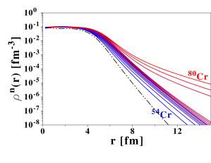
Figure 20: (Color Online) Neutron densities for even-even Cr isotopes, from ⁵⁴Cr to ⁸⁰Cr. The proton density of ⁵⁴Cr is given (dashed-dotted line) as a reference for the neutron skin.

The halo factor $\delta{R}_{\mathrm{halo}}$ is shown in Fig. 21 as a function of $A/N$. The halo contributes significantly to the total neutron r.m.s. radius (up to $\sim 0.13$ fm) beyond the $N=50$ shell closure.

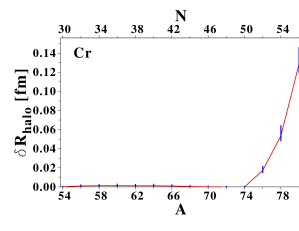
Figure 21: (Color Online) Halo factor parameter $\delta{R}_{\mathrm{halo}}$ in the Cr isotopic chain.

The latter result can be recast as a splitting of the total r.m.s. radius into a core and a halo contributions, as displayed in Fig. 22. In contrast to the Helm model, shell effects are here properly separated from halo ones, e.g. the core r.m.s. radius includes a kink at $N=50$ which is due to the filling of least bound states and not to the halo per se. Only the physics related to the existence of truly decorrelated neutrons is extracted by $N_{\mathrm{halo}}$ and $\delta R_{\mathrm{halo}}$. The kink of the neutron r.m.s radius (i) was not assumed as a halo signature a priori Meng and Ring (1998); Meng et al. (2002) but recovered a posteriori (ii) must be corroborated using finer tools such as $N_{\mathrm{halo}}$ and $\delta R_{\mathrm{halo}}$ to extract quantitatively the contribution of the halo to that kink.

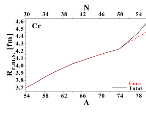
Figure 22: (Color Online) Total neutron root-mean-square radius (solid line) and core contribution (dashed line) for chromium isotopes, as predicted by the {SLy4+REG-M} functional.

To characterize further this halo region, individual contributions $N_{\mathrm{halo,i}}$ are evaluated. The results are summarized in Tab. 2. As expected, the main contributions to the halo come from the most weakly-bound states, while for non-halo nuclei, like ⁷⁴Cr, all contributions are consistent with zero. At the neutron drip-line, important contributions are found from both $3s_{1/2}$ and $2d_{5/2}$ states. The latter $\ell=2$ states contribute for almost $50\%$ of the total number of nucleons in the decorrelated region, although this state is more localized than the $3s_{1/2}$ because of its binding energy and of the effect of the centrifugal barrier. Such hindrance effects are compensated by the larger canonical occupation of the $d_{5/2}$ states and the larger intrinsic degeneracy of the shell. The significant contribution of the $\ell=2$ states could not be expected from the standard qualitative analysis presented in Sec. II.2 or, with a few exceptions Kanungo et al. (2002), from the experience acquired in light nuclei.

	74Cr
$N_{\mathrm{halo}}$	$1.7.10^{-4}$
	$e^{n}_{i}$ [MeV]	$v_{i}^{n\,2}$	$N_{\mathrm{halo,i}}$	$P_{i}$
$3s_{1/2}$	$+0.036$	$0.000$	$0.000$	$0.0\%$
$2d_{5/2}$	$-0.024$	$0.000$	$0.000$	$0.0\%$
$1g_{9/2}$	$-3.618$	$1.000$	$0.001$	$0.1\%$
$2p_{1/2}$	$-8.100$	$1.000$	$0.000$	$0.0\%$
$1f_{5/2}$	$-8.400$	$1.000$	$0.000$	$0.0\%$
$Other$	$<-10.0$	—	$\sim 1.7.10^{-4}$	—
	76Cr
$N_{\mathrm{halo}}$	$5.2.10^{-2}$
	$e^{n}_{i}$ [MeV]	$v_{i}^{n\,2}$	$N_{\mathrm{halo,i}}$	$P_{i}$
$3s_{1/2}$	$+0.356$	$0.050$	$0.007$	$14.8\%$
$2d_{5/2}$	$-0.209$	$0.311$	$0.039$	$12.6\%$
$1g_{9/2}$	$-3.764$	$0.991$	$0.002$	$0.2\%$
$2p_{1/2}$	$-8.416$	$0.998$	$0.000$	$0.0\%$
$1f_{5/2}$	$-8.477$	$0.998$	$0.000$	$0.0\%$
$Other$	$<-10.0$	—	$\sim 2.2.10^{-3}$	—
	78Cr
$N_{\mathrm{halo}}$	$0.186$
	$e^{n}_{i}$ [MeV]	$v_{i}^{n\,2}$	$N_{\mathrm{halo,i}}$	$P_{i}$
$3s_{1/2}$	$+0.052$	$0.147$	$0.045$	$30.4\%$
$\mathbf{2d_{5/2}}$	$\mathbf{-0.450}$	$\mathbf{0.604}$	$\mathbf{0.128}$	$\mathbf{21.2\%}$
$1g_{9/2}$	$-3.919$	$0.991$	$0.005$	$0.5\%$
$1f_{5/2}$	$-8.576$	$0.998$	$0.001$	$0.1\%$
$2p_{1/2}$	$-8.714$	$0.998$	$0.001$	$0.1\%$
$Other$	$<-10.0$	—	$\sim 6.2.10^{-3}$	—
	80Cr
$N_{\mathrm{halo}}$	$0.450$
	$e^{n}_{i}$ [MeV]	$v_{i}^{n\,2}$	$N_{\mathrm{halo,i}}$	$P_{i}$
$\mathbf{3s_{1/2}}$	$\mathbf{-0.178}$	$\mathbf{0.421}$	$\mathbf{0.207}$	$\mathbf{49.3\%}$
$\mathbf{2d_{5/2}}$	$\mathbf{-0.670}$	$\mathbf{0.843}$	$\mathbf{0.223}$	$\mathbf{26.4\%}$
$1g_{9/2}$	$-4.062$	$0.995$	$0.008$	$0.8\%$
$1f_{5/2}$	$-8.676$	$0.999$	$0.001$	$0.1\%$
$2p_{1/2}$	$-8.942$	$0.999$	$0.002$	$0.2\%$
$Other$	$<-10.0$	—	$\sim 9.4.10^{-2}$	—

Table 2: Contributions of the least bound canonical orbitals to the number of nucleons in the decorrelated region, and probabilities for those states to be in the outer region $r\geq r_{0}$. The data are provided for the four last (predicted) bound Cr isotopes.

Finally, the probability $P_{i}$ for nucleons occupying the canonical state $\phi^{n}_{i}$ to be in the outer region $r\geq r_{0}$ in ⁸⁰Cr is typical of $s-$wave halo systems; i.e. $49\%$ for the $3s_{1/2}$ state and a little bit lower for the $2d_{5/2}$ state, around $26\%$.

The analysis method applied to neutron-rich Cr isotopes demonstrates unambiguously that a halo is predicted for the last three bound isotopes. We have indeed been able to characterize the existence of a decorrelated region in the density profile for isotopes beyond the $N=50$ shell closure. Such a region contains a small fraction of neutrons which impact significantly the extension of the nucleus. It is generated by an admixture of $s_{1/2}$ and $d_{5/2}$ states, whose probabilities to be in the halo region $r\geq r_{0}$ are compatible with what is seen in light halo nuclei. This provides the picture of a rather collective halo building up at the neutron drip-line for Cr isotopes.

V.3 Sn isotopes

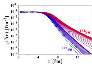
Figure 23: (Color Online) Same as Fig. 20 for the Sn isotopes. The ”separation” between the two groups of neutron densities occurs for $N=82$. Proton density of ¹⁰⁰Sn is given as a reference in dashed-dotted line.

So far, the prediction of halos in tin isotopes beyond the $N=82$ shell closure Mizutori et al. (2000) have been based on the Helm model, whose limitations have been pointed out in Sec. III.2.2. The robust analysis tools introduced in the present work are expected to give more reliable results. Neutron densities of Sn isotopes do exhibit a qualitative change for $N>82$, as seen in Fig. 23. However, the transition is smoother than in the case of chromium isotopes (Fig. 20). This is partly due the increase of collectivity associated with the higher mass. There are also specific nuclear-structure features that explain the absence of halo in drip-line Sn isotopes.

Tab. 3 displays the canonical and quasiparticle spectra for the drip-line nucleus ¹⁷⁴Sn. The energy scales at play are not compliant with the definition of a halo, as can also be seen from Fig. 24. In the canonical basis, the separation energy $E$ is roughly $1.2$ MeV, whereas six states with an energy spread $\Delta E\approx 3.8$ MeV are separated from a core of orbitals by a gap $E^{\prime}\approx 5.5$ MeV. Equivalently in the quasiparticle basis one has (i) $S_{n}=E\approx 1.5$ MeV, (ii) four low-lying quasiparticles with a spread $\Delta E\approx 3.4$ MeV (iii) separated from higher excitations by $E^{\prime}\approx 5.6$ MeV. The energy spread of the low-lying states $\Delta E$ is too large to favor the formation of a halo. Also, according to the phenomenological criterion extracted for light halo nuclei, the separation energy of ¹⁷⁴Sn should have been of the order of $2$ MeV$/A^{2/3}\approx 64$ keV for a halo to emerge.

Can. spectrum 174			Exc. spectrum 173Sn
		$e^{n}_{i}$ [MeV]			$E^{n}_{\nu}-\lambda^{n}$ [MeV]
————		$>0$			$>15$
$E\left\updownarrow\vphantom{\begin{array}[]{l}a\\ a\\ a\end{array}}\right.\!\!$				$d_{5/2}$	14.169
				$d_{3/2}$	12.026
				$s_{1/2}$	11.967
$\Delta E\left\{\vphantom{\begin{array}[]{l}a\\ a\\ a\\ a\\ a\\ a\end{array}}\right.$	$1i_{13/2}$	-1.208		$1h_{11/2}$	10.603
	$3p_{1/2}$	-1.855	$E^{\prime}\left\updownarrow\vphantom{\begin{array}[]{l}a\\ a\\ a\\ a\end{array}}\right.\!\!$
	$2d_{5/2}$	-2.227
	$3p_{3/2}$	-2.665
	$1h_{9/2}$	-3.823
	$2f_{7/2}$	-5.014	$\Delta E\left\{\vphantom{\begin{array}[]{l}a\\ a\\ a\\ a\\ a\\ a\\ a\\ a\\ a\\ a\\ a\end{array}}\right.$	$f_{7/2}$	4.937
$E^{\prime}\left\updownarrow\vphantom{\begin{array}[]{l}a\\ a\\ a\\ a\\ a\\ a\\ a\\ a\end{array}}\right.\!\!$				$f_{7/2}$	4.463
				$h_{9/2}$	3.890
				$p_{3/2}$	2.722
				$p_{1/2}$	2.648
				$p_{3/2}$	2.559
				$f_{5/2}$	2.290
				$f_{5/2}$	2.082
				$p_{1/2}$	1.905
	$1h_{11/2}$	-10.575		$p_{1/2}$	1.610
	$2d_{3/2}$	-12.581		$i_{13/2}$	1.502
	$3s_{1/2}$	-12.747	$E\left\updownarrow\vphantom{\begin{array}[]{l}a\\ a\end{array}}\right.\!\!$
	$2d_{5/2}$	-14.944
		$<-15$	————		$0$

Table 3: Same as Tab. 1 for the neutron canonical energies of ¹⁷⁴Sn, and associated separation energies $|\epsilon^{n}_{\nu}|$ of ¹⁷³Sn.

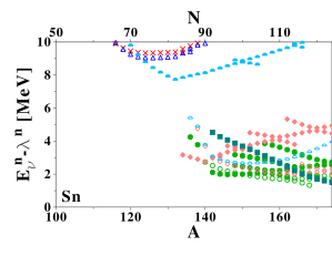
Figure 24: (Color Online) Same as Fig. 18 for neutron separation energies of Sn isotopes.

	132Sn
$N_{\mathrm{halo}}$	$0.13.10^{-2}$
	$e^{n}_{i}$ [MeV]	$v_{i}^{n\,2}$	$N_{\mathrm{halo,i}}$	$P_{i}$
$1i_{13/2}$	$+2.648$	$0.000$	$0.000$	$0.0\%$
$3p_{1/2}$	$+2.489$	$0.000$	$0.000$	$0.0\%$
$2f_{5/2}$	$+1.661$	$0.000$	$0.000$	$0.0\%$
$3p_{3/2}$	$+1.240$	$0.000$	$0.000$	$0.0\%$
$1h_{9/2}$	$+1.141$	$0.000$	$0.000$	$0.0\%$
$2f_{7/2}$	$-1.785$	$0.000$	$0.000$	$0.0\%$
$Other$	$<-7.0$	—	$\sim 0.13.10^{-2}$	—
	146Sn
$N_{\mathrm{halo}}$	$0.71.10^{-1}$
	$e^{n}_{i}$ [MeV]	$v_{i}^{n\,2}$	$N_{\mathrm{halo,i}}$	$P_{i}$
$1i_{13/2}$	$+1.435$	$0.064$	$0.000$	$0.2\%$
$2f_{5/2}$	$-0.056$	$0.155$	$0.004$	$2.4\%$
$3p_{1/2}$	$-0.202$	$0.143$	$0.005$	$3.8\%$
$1h_{9/2}$	$-0.401$	$0.262$	$0.001$	$0.3\%$
$3p_{3/2}$	$-1.050$	$0.442$	$0.040$	$9.0\%$
$2f_{7/2}$	$-3.037$	$0.923$	$0.017$	$1.9\%$
$Other$	$<-7.0$	—	$\sim 3.1.10^{-3}$	—
	164Sn
$N_{\mathrm{halo}}$	$0.179$
	$e^{n}_{i}$ [MeV]	$v_{i}^{n\,2}$	$N_{\mathrm{halo,i}}$	$P_{i}$
$1i_{13/2}$	$-0.216$	$0.349$	$0.002$	$0.5\%$
$3p_{1/2}$	$-1.347$	$0.804$	$0.052$	$6.6\%$
$2f_{5/2}$	$-1.481$	$0.155$	$0.032$	$4.0\%$
$3p_{3/2}$	$-2.143$	$0.923$	$0.072$	$7.8\%$
$1h_{9/2}$	$-2.503$	$0.894$	$0.003$	$0.4\%$
$2f_{7/2}$	$-4.301$	$0.975$	$0.014$	$1.4\%$
$Other$	$<-7.0$	—	$\sim 4.7.10^{-3}$	—
	174Sn
$N_{\mathrm{halo}}$	$0.149$
	$e^{n}_{i}$ [MeV]	$v_{i}^{n\,2}$	$N_{\mathrm{halo,i}}$	$P_{i}$
$1i_{13/2}$	$-1.208$	$0.872$	$0.005$	$0.5\%$
$3p_{1/2}$	$-1.854$	$0.979$	$0.049$	$5.0\%$
$2f_{5/2}$	$-2.227$	$0.977$	$0.028$	$2.9\%$
$3p_{3/2}$	$-2.665$	$0.989$	$0.054$	$5.5\%$
$1h_{9/2}$	$-3.823$	$0.989$	$0.002$	$0.2\%$
$2f_{7/2}$	$-5.014$	$0.996$	$0.009$	$0.9\%$
$Other$	$<-7.0$	—	$\sim 2.3.10^{-3}$	—

Table 4: Same as Tab. 2 for Sn isotopes.

The $N_{\mathrm{halo}}$ parameter is displayed in Fig. 25. The maximum value of $N_{\mathrm{halo}}$, around $0.18$, is very small compared to the total number of nucleons. The absolute numbers are also smaller than the ones obtained in (lighter) Cr halos. We may add that the value of $N_{\mathrm{halo}}$ found here is of the same order of magnitude as those encountered for a non-halo $p$-wave nucleus such as ¹³N, where around $0.12$ neutron out of six reside in average in the classically forbidden region Nunes . An interesting feature is the decrease of $N_{\mathrm{halo}}$ for $N>166$. This is a consequence of the filling of the highly degenerate $1i_{13/2}$ state right at the drip-line (see Fig. 5). As the number of neutrons occupying the $1i_{13/2}$ shell increases, the depth of the one-body potential also increases and the shells become more bound, thus more localized. As this happens over a significant number of neutrons, the effect on $N_{\mathrm{halo}}$ is visible. This constitutes an additional hindrance to the formation of halos from low-lying high angular-momentum states.

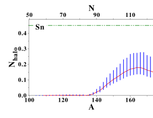
Figure 25: (Color Online) Average number of nucleons in the spatially decorrelated region for Sn isotopes. For comparison, $N_{\mathrm{halo}}(^{80}$Cr$)$ is shown as a horizontal dashed-dotted line.

The second halo parameter $\delta{R}_{\mathrm{halo}}$ displayed in Fig. 26 shows that the decorrelated region has little influence on the nuclear extension, of the order of $0.02$ fm. Its contribution is found to be much less than predicted by the Helm model. The heavy mass of tin isotopes hinders the possibility of a sharp separation of core and tail contributions in the total density and thus, of the formation of a halo.

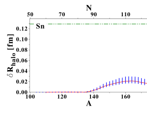
Figure 26: (Color Online) Halo factor parameter $\delta{R}_{\mathrm{halo}}$ in the Sn isotopic chain. For comparison purposes, the maximum value of $\delta R_{\mathrm{halo}}$ obtained for Cr isotopes is represented as a horizontal dashed-dotted line.

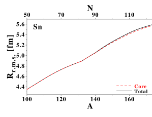
Figure 27: (Color Online) Same as Fig. 22 for Sn isotopes.

The analysis of single-particle contributions, summarized in Tab. 4, confirms the latter analysis. First, $3p_{1/2}$, $3p_{3/2}$ and $2f_{7/2}$ ($\ell=3$) states contribute roughly the same to $N_{\mathrm{halo}}$. For higher angular-momentum orbitals, the effect of the centrifugal barrier is seen: the $1h_{9/2}$ and $1i_{13/2}$ orbitals, the latter being the least bound orbital, do not contribute significantly to the decorrelated region. Finally, individual probabilities $P_{i}$ remain very small, and do not exceed a few percent.

For all the reasons exposed above, only a neutron skin effect is seen in tin isotopes, and no significant halo formation is envisioned. Of course, all results presented here have been obtained with a particular EDF and it is of interest to probe the sensitivity of the predictions to the different ingredients of the method Rotival et al. .

In any case, the two previous examples already provide a coherent picture regarding the properties of halo or non-halo medium-mass nuclei. In particular, it is rather obvious that the notion of giant halo Meng and Ring (1998); Sandulescu et al. (2003); Geng et al. (2004); Kaushik et al. (2005); Grasso et al. (2006); Terasaki et al. (2006) constituted of six to eight neutrons is misleading. Indeed, such a picture was obtained by summing up the total occupations of loosely bound orbitals. Although loosely bound orbitals are indeed responsible for the formation of the halo, nucleons occupying them still reside mostly inside the nuclear volume. It is thus unappropriate to simply sum up their occupations to characterize the halo. The identification of the halo region in the presently proposed method led us to define the more meaningful quantity $N_{\mathrm{halo}}$.

VI Conclusions

The formation of halo in finite many-fermion systems is a quantum phenomenon caused by the possibility for non-classical systems to expand in the classically forbidden region. One difficulty to further understand this phenomenon resides in the absence of tools to characterize halo properties in a quantitative way. Light nuclei constitute an exception considering that the quantification of halo properties in terms of the dominance of a cluster configuration and of the probability of the weakly-bound clusters to extend beyond the classical turning point is well acknowledged Fedorov et al. (1993); Jensen and Riisager (2000); Riisager et al. (2000); Jensen and Zhukov (2001). Several attempts to characterize halos in systems constituted of tens of fermions have been made but were based on loose definitions and quantitative criteria. Such a situation is unsatisfactory because important questions, such as the very existence of halos at the neutron drip-line of medium-mass nuclei, are still open.

After demonstrating the inability of the Helm model to provide reliable predictions, a new quantitative analysis method has been developed to identify and characterize halos in finite many-fermion systems in a model-independent fashion. It is based on the decomposition of the internal one-body density in terms of overlap functions. The definition of the halo, as a region where nucleons are spatially decorrelated from the others, has been shown to be connected to specific patterns of the internal one-body density and of the energy spectrum of the $(N-1)$-body system. In particular, halos can be characterized by the existence of a small nucleon separation energy $E$, a small energy spread $\Delta E$ of low-lying excitations, and a large excitation energy $E^{\prime}$ of the upper-lying states with respect to low-lying bunched ones, in the excitation spectrum of the $(N-1)$-body system.

Based on the new analysis method, it is possible to extract the radius $r_{0}$ beyond which the halo, if it exists, dominates over the core. Such an identification of $r_{0}$ has been validated by extensive simulations. It is important to stress that the method does not rely on an a priori separation of the density into core and halo components. The latter are extracted from the analysis itself, using the total matter density as the only input. Several quantitative observables are then introduced, namely (i) the average number of fermions participating in the halo, (ii) the influence of the halo region on the total extension of the system, and (iii) the contributions of individual overlap functions to the halo.

The new analysis method has been applied to the results obtained from energy density functional calculations of chromium and tin isotopes using the code HFBRAD Bennaceur and Dobaczewski (2005). Drip-line Cr isotopes appear as ideal halo candidates whereas tin isotopes do not.

For drip-line Cr isotopes, the average fraction of nucleon participating in the halo is of the order of $\sim 0.5$. Such a value is compliant with those found for light halo systems Nunes . The halo region was also found to influence significantly the nuclear extension. Contributions from several individual components, including $\ell=2$ ones, were identified, contradicting the standard picture arising from few-body models. The notion of collective halos in medium-mass nuclei has been introduced.

In the case of Sn isotopes, the average number of nucleons participating in the halo is very small and has no influence on the nuclear extension. Thus, the drip-line phenomenon discussed previously for tin isotopes Mizutori et al. (2000) is rather a pronounced neutron skin effect. Such skin effects are of course of interest as they emphasize the isovector dependence of the energy density functionals. However, they should not be confused with halo systems which display an additional long tail of low density matter.

This preliminary study on two isotopic series gives promising results and validates the theoretical grounds of the analysis. With upcoming new radioactive beam facilities, interaction cross-sections are expected to be measurable in the drip-line region of $Z\approx 26$ elements whi (2006). This would constitute a giant leap towards an extensive comparison between theoretical and experimental works on drip-line physics.

Appendix A Internal one-body density

A.1 Definition

In the laboratory frame, the one-body density is the expectation value of the operator

$$\hat{\rho}(\vec{r}\,)=\sum_{i=1}^{N}\,\delta(\vec{r}-\hat{\vec{r}}_{i})\,,$$ (37)

which leads for the $N$-body ground state to

$$\!\!\!\!\rho(\vec{r}\,)\! = \!N\!\!\int d\vec{r}_{1}\ldots d\vec{r}_{N-1}\,|{\Psi}^{N}_{0}(\vec{r}_{1}\ldots\vec{r}_{N-1},\vec{r}\,)|^{2}$$ (38)

$$= \!N\!\!\int d\vec{\xi}_{1}\ldots d\vec{\xi}_{N-2}\,d\vec{R}_{N-1}$$

$$\leavevmode\nobreak\ \leavevmode\nobreak\ \leavevmode\nobreak\ \leavevmode\nobreak\ \leavevmode\nobreak\ \leavevmode\nobreak\ \leavevmode\nobreak\ \leavevmode\nobreak\ \times|{\tilde{\Phi}}^{N}_{0}(\vec{\xi}_{1}\ldots\vec{\xi}_{N-2},\vec{r}-\vec{R}_{N-1})|^{2}\,\,\,$$

where $\Phi^{N}_{i}(\vec{r}_{1}\ldots\vec{r}_{N})\equiv\tilde{\Phi}^{N}_{i}(\vec{\xi}_{1}\ldots\vec{\xi}_{N-1})$. Using that $\tilde{\Phi}^{N}_{i}$ is invariant under translation of the system, one easily proves that the one-body density in the laboratory frame is also translationally invariant, $\rho(\vec{r}+\vec{a}\,)=\rho(\vec{r}\,)$, and thus is uniform. This is a general property of translationally invariant systems which underlines that the density in the laboratory frame is not the proper tool to study self-bound systems.

The relevant object for self-bound systems is the internal one-body density matrix, defined as the expectation value of the operator

$$\hat{\rho}_{\mathrm{[1]}}(\vec{r},\vec{r}\,^{\prime})=\delta(\vec{R}_{N})\sum_{i=1}^{N}\delta(\vec{r}-\hat{\vec{r}}_{i}+\hat{\vec{R}}_{N-1}^{\,i})\\ \times\delta(\vec{R}\,^{\prime}_{N})\sum_{j=1}^{N}\delta(\vec{r}\,^{\prime}-\hat{\vec{r}}\,^{\prime}_{j}+\hat{\vec{R}}_{N-1}^{\,j^{\prime}})\\ \times\prod_{\begin{subarray}{c}k,l=1..N\\ k,l\neq i,j\end{subarray}}\delta(\hat{\vec{r}}_{k}-\hat{\vec{r}}_{l})\,,$$ (39)

where

$$\hat{\vec{R}}_{N-1}^{\,i}=\frac{1}{N-1}\sum_{\begin{subarray}{c}j=1\\ j\neq i\end{subarray}}^{N}\hat{\vec{r}}_{j}\,.$$ (40)

The internal density defined with respect to the center-of-mass of the remaining $(N-1)$-body⁽⁾ is of direct relevance to knockout reactions Clément (1973a, b); Dieperink and de Forest, Jr. (1974). Using the orthogonality relationship Van Neck et al. (1996)

$$\int\,d\vec{r}_{1}\ldots d\vec{r}_{N}\,{{\Phi}^{N}_{i}}^{*}(\vec{r}_{1}\ldots\vec{r}_{N})\,\delta(\vec{R}_{N})\,{\Phi}^{N}_{j}(\vec{r}_{1}\ldots\vec{r}_{N})=\delta_{ij}\,\,,$$ (41)

and (21), one obtains Van Neck et al. (1993); Van Neck and Waroquier (1998); Shebeko et al. (2006)

$$\rho_{\mathrm{[1]}}(\vec{r},\vec{r}\,^{\prime}) = N\int d\vec{r}_{1}\ldots d\vec{r}_{N-1}\,{{\Phi}^{N}_{0}}^{*}(\vec{r}_{1}\ldots\vec{r}_{N-1},\vec{r}\,^{\prime})$$ (42)

$$\leavevmode\nobreak\ \leavevmode\nobreak\ \leavevmode\nobreak\ \leavevmode\nobreak\ \leavevmode\nobreak\ \leavevmode\nobreak\ \times\delta(\vec{R}_{N-1}){\Phi}^{N}_{0}(\vec{r}_{1}\ldots\vec{r}_{N-1},\vec{r}\,)$$

$$= \sum_{\nu}\varphi^{*}_{\nu}(\vec{r}\,^{\prime})\varphi_{\nu}(\vec{r}\,)\,,$$

which shows that the internal one-body density matrix is completely determined by internal overlap functions Van Neck et al. (1993).

The internal one-body density $\rho_{\mathrm{[1]}}(\vec{r}\,)$ is the local part of the internal density matrix, and is the expectation value of the operator

$$\hat{\rho}_{\mathrm{[1]}}(\vec{r}\,)=\delta(\vec{R}_{N})\sum_{i=1}^{N}\delta(\vec{r}-\hat{\vec{r}}_{i}+\hat{\vec{R}}_{N-1}^{\,i})\,.$$ (43)

According to Eq. (42), one has

$$\rho_{\mathrm{[1]}}(\vec{r}\,)=\sum_{\nu}|\varphi_{\nu}(\vec{r}\,)|^{2}=\sum_{\nu}\frac{2\ell_{\nu}+1}{4\pi}|\bar{\varphi}_{\nu}(r)|^{2}\,.$$ (44)

A.2 Nuclear EDF calculations

The behavior of the internal one-body density highlighted in Sec. IV is general and model-independent. It is valid for any finite many-fermion system, as long as the inter-fermion interaction is negligible beyond a certain relative distance. Of course, when an approximate treatment of the $N$-body system is used, a certain deterioration of the properties of the density can be observed. In the case of EDF calculations however, some more profound issues are raised.

First, an important clarification regarding the physical interpretation of the quantities at play in the calculations must be carried out. In single-reference implementations of the nuclear EDF method, one manipulates the so-called ”intrinsic” one body density, in the sense that it is built from an auxiliary state that breaks symmetries of the nuclear Hamiltonian, e.g. translational, rotational and gauge invariance. The intrinsic density is associated with a wave packet from which true eigenstates, and their laboratory and internal densities, can be recovered by restoring broken symmetries through multi-reference EDF calculations Bender et al. (2003). In practice, the intrinsic density is used as a good approximation to the internal density, e.g. when analyzing electron scattering data. Still, the intrinsic density of a symmetry breaking state and the internal density associated with the true eigenstate of interest are different⁽⁾ Giraud (2008). As a result, EDF methods⁽⁾ Engel (2007). expressed directly in terms of the internal density are currently being considered Engel (2007).

As just said, the EDF intrinsic density has been shown in many cases to be a good approximation of the internal density extracted through electron scattering. In practice, one identifies the lower component of the intrinsic HFB wave-function $V^{q}_{\nu}(\vec{r}\,)$ with the internal overlap function $\varphi^{q}_{\nu}(\vec{r}\,)$ leading from the ground state of the $N$-body system to the corresponding excited state of the $(N-1)$-body system⁽⁾. In particular, and this is key to the present discussion, the asymptotic part of $V^{n}_{\nu}(\vec{r}\,)$ satisfies the free Schrödinger equation Bennaceur and Dobaczewski (2005), just as the asymptotic part of $\varphi^{n}_{\nu}(\vec{r}\,)$ does. The smallest energy $|\epsilon^{n}_{0}|$ thus extracted relates to the exact separation energy, i.e. an analogue to Koopmans’ theorem derived originally in the case of Hartree-Fock approximation applies. Given that the intrinsic density (Eq. 36) expressed in terms of the lower component of HFB quasiparticle wave-functions reads the same as the internal density expressed in terms of overlap functions (Eq. 44), the analysis method developed in Sec. IV, including the occurrence of crossing patterns, applies directly to the former.

A.2.1 Slater determinant as an auxiliary state

In the implementation of the EDF method based on a Slater determinant, explicit spectroscopic factors are either zero or one, and behave according to a step function $S^{q}_{\nu}=\Theta(\epsilon^{q}_{F}-e^{q}_{\nu})$. The single-particle orbitals $\varphi^{q}_{\nu}$ are identified with overlap functions and the density takes the form given by Eq. (44).

A.2.2 Quasiparticle vacuum as an auxiliary state

In the implementation of the EDF method based on a quasiparticle vacuum, the one-body density can be evaluated using either the canonical states $\phi^{q}_{i}$ or the lower components $V^{q}_{\nu}$ of the quasiparticle states

$$\rho^{q}(r)=\sum_{i}\frac{2j^{q}_{\nu}+1}{4\pi}v^{q\,2}_{i}|\bar{\phi}^{q}_{i}(r)|^{2}=\sum_{\nu}\frac{2j^{q}_{\nu}+1}{4\pi}|\bar{V}^{q}_{\nu}(r)|^{2}\,\,,$$ (45)

where $j^{q}$ relates to the total angular momentum. In the present case, the spectroscopic factor $S^{q}_{\nu}$ identifies with the quasiparticle occupation $N^{q}_{\nu}$ defined by Eq. (7). This underlines that implementation of the EDF approach based on a quasiparticle vacuum incorporates explicitly parts of the spreading of the single-particle strength Van Neck et al. (2006).

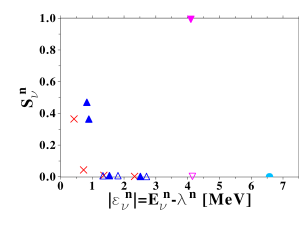
Figure 28: (Color Online) Neutron quasiparticle occupation $N^{n}_{\nu}$ as a function of the separation energy in ⁸⁰Cr, calculated with the {SLy4+REG-M} functional. Conventions from Fig. 2 are used to label individual quasiparticle states. Only quasiparticles with occupations greater than $10^{-3}$ are displayed.

The function $S^{n}_{\nu}=f(|\epsilon^{n}_{\nu}|)$, whose typical behavior is presented in Fig. 28 for ⁸⁰Cr, takes values between zero and one. The difference between hole-like quasiparticle excitations and particle-like ones is visible. Indeed, $S^{n}_{\nu}$ increases with excitation energy $|\epsilon^{n}_{\nu}|$ for hole-like excitations. This constitutes the main branch which tends towards a step function when correlations are not explicitly included into the auxiliary state; i.e. for the EDF approach based on an auxiliary Slater determinant. Spectroscopic factors of particle-like quasiparticle excitations remain small and go to zero for high-lying excitations.

Appendix B Determination of the halo region

Let us start with a very crude toy model, where everything is analytical. The total density $\rho$ is assumed to be a superposition of a core $\rho_{c}$ and a tail $\rho_{h}$, both taking the form

$$\rho_{i}(r)=A_{i}\,\kappa_{i}\,e^{-\kappa_{i}\,r}\,.$$ (46)

This amounts to considering that the asymptotic regime is reached in the region of the crossing between $\rho_{c}$ and $\rho_{h}$, and we neglect for now the $r^{-2}$ factor. In this model the second-order (base-$10$) log-derivative of the total density is analytical, as well as the exact positions of (i) its maximum $r_{\mathrm{max}}$ (ii) the point $r_{0}$ where the halo density is exactly equal to ten times the core one. Then, the ratio $\mathcal{R}(r_{0})=\log_{10}^{\prime\prime}\rho(r_{0})/\log_{10}^{\prime\prime}\rho(r_{\mathrm{max}})$ can be evaluated and becomes in the weak binding limit of interest $\kappa_{h}/\kappa_{c}\rightarrow 0$

$$\mathcal{R}(r_{0})\underset{\kappa_{h}/\kappa_{c}\rightarrow 0}{\longrightarrow}\frac{40}{121}+\mathcal{O}\left[\left(\frac{\kappa_{h}}{\kappa_{c}}\right)^{2}\right]\,.$$ (47)

This shows that the position where there is a factor of ten between $\rho_{c}$ and $\rho_{h}$ is equivalently obtained by finding the position where there is a given ratio between the value of the second-order log-derivative of the density and its maximal value. The critical value $40/121\approx 0.33$ found in the toy model is not believed to be accurate for complex nuclei, as (i) the asymptotic regime is not reached at the crossing point and is more complicated because of the $r^{-2}$ factor (ii) the total density is a superposition of more than two components. However, we expect the one-to-one correspondence between ratios on the densities and ratios on $\log_{10}^{\prime\prime}\rho$ to hold in realistic cases. Thus, the position where the halo dominates the core by one order of magnitude can be found using $\log_{10}^{\prime\prime}\rho$ as the only input.

More realistic model calculations have been used to characterize the position of $r_{0}$. The total density is taken as a linear combination of core and halo contributions. Their relative normalization are free parameters in this simulation, allowing to artificially change the fraction of halo in the total density

$$\rho_{\mathrm{tot}}(r)=\displaystyle N_{c}\,\rho_{c}(r)+\sum_{\nu=1}^{m}N_{\nu}\,\rho_{\nu}(r)\,,$$ (48)

where $N_{c}$ and $\displaystyle N_{h}=\sum_{\nu=1}^{m}N_{\nu}$ are the number of nucleons in the core part and in the halo part, respectively. The densities $\rho_{c}$ and $\rho_{\nu}$ are normalized to one. We considered (i) simple models, where the core and each halo components are defined as

$$\left\{\begin{array}[]{lcl}\displaystyle\rho_{i}(r)=\frac{1}{\mathcal{N}_{i}}&&r<R_{0}\,,\\ \\ \displaystyle\rho_{i}(r)=\frac{1}{\mathcal{N}_{i}}e^{\frac{R_{0}-r}{a_{i}}}&&r>R_{0}\,,\end{array}\right.$$ (49)

$\mathcal{N}_{i}$ standing for a normalization constant. This model only accounts for the basic features of the nuclear density: a uniform core of radius $R_{0}$ and a spatial extension becoming larger as $a_{i}\rightarrow 0$ (ii) double Fermi models, where the un-physical sharp edge in the logarithmic representation of the previous density is smoothened out

$$\rho_{i}(r)=\frac{\rho_{0}}{1+e^{\frac{r-R_{0}}{a_{i}}}}$$ (50)

(iii) semi-phenomenological models, which fulfill the asymptotic behavior of Eq. (28). Core and tail densities vanish at $r=0$, as well as their derivatives with respect to $x$, $y$ and $z$, in order to avoid singularities at the nucleus center Berdichevsky and Mosel (1982). In Refs. Gambhir and Patil (1985, 1986); Bhagwat et al. (2000), such densities were adjusted on experimental data. The core part was defined as

$$\rho_{c}(r)=\frac{\rho_{0,c}}{1+\left[\frac{1+\left(\frac{r}{R_{0,c}}\right)^{2}}{2}\right]^{\alpha}\left[e^{\frac{r-R_{0,c}}{a_{c}}}+e^{\frac{-r-R_{0,c}}{a_{c}}}\right]}\,\,,$$ (51)

where $\alpha=1$ for neutrons, and the halo density as

$$\rho_{h}(r)=\rho_{0,t}\left[\frac{r^{2}}{\left(r^{2}+R_{0,t}^{2}\right)}\right]e^{-\frac{r}{a_{t}}}\,\,,$$ (52)

(iv) more realistic models, where the core density is still defined as in Eq. (51), but the halo contributions are realistic wave functions taken from self-consistent EDF calculations of Cr and Sn isotopes.

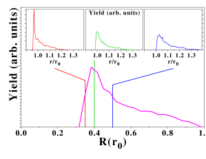
Figure 29: (Color Online) [Main panel] Ratio between the second-order log-density at $r_{0}$ and its peak value $\log_{10}^{\prime\prime}\rho(r_{\mathrm{max}})$ [Top panels] Distribution of $r/r_{0}$ for which $\mathcal{R}(r)$ is equal to a given value (left panel: $\mathcal{R}(r)=0.35$, middle panel: $\mathcal{R}(r)=0.4$, right panel: $\mathcal{R}(r)=0.5$), and $r_{0}$.

The results from a wide panel of test cases are presented in Fig. 29. We recall that $r_{0}$ is defined as the radius for which $\rho_{h}(r_{0})=10\rho_{c}(r_{0})$. The goal is to determine such a radius through the value of another ratio: $\mathcal{R}(r_{0})$. For each simulation, the position $r_{0}$ and the ratio $\mathcal{R}(r_{0})$ are computed. The main panel of Fig. 29 shows the distribution of $\mathcal{R}(r_{0})$ which is peaked around $0.4$. This value is greater than in the toy model case for the reasons detailed above. The distribution of $\mathcal{R}(r_{0})$ is asymmetric, but the tail towards high values corresponds precisely to non-halo systems. In any case, we are going to reflect such an asymmetry into the choice of theoretical uncertainties in the determination of $r_{0}$.

The inserts of Fig. 29 display the distribution of ratio $r/r_{0}$ corresponding to a given value of $\mathcal{R}(r)$. The ratio $\mathcal{R}(r)=2/5$ (top-center panel) indeed picks out quite consistently the radius $r_{0}$. For $\mathcal{R}(r)=40/121$ (top-left panel), the position $r$ is in most cases below $r_{0}$. As a consequence, the average ratio between tail and core components in the density will be consistently below ten in this case. On the contrary for $\mathcal{R}(r)=1/2$ (top-right panel), $r$ is systematically larger than $r_{0}$, meaning that the $\rho_{h}/\rho_{c}$ larger than ten on the average. In the end, it appears that $r_{0}$ is indeed well picked out through the condition

$$\mathcal{R}(r_{0})=\frac{2}{5}\,.$$ (53)

For those reasons, we use those values of $\mathcal{R}(r)$ to set the error bars on the determination of $r_{0}$.

Of course, we need to account for the fact that a difference by one order of magnitude between core and halo densities to define the halo region is somewhat arbitrary and that the corresponding radius $r_{0}$ cannot be perfectly picked out in all cases through Eq. (53). As a result, we add a tolerance margin to the definition of $r_{0}$ by allowing $\mathcal{R}(r_{0})$ to vary between $40/121\approx 0.35$ and $1/2$. The upper margin is greater than the lower one to account for the asymmetry of the peak in Fig. 29. Note that the procedure chosen to determine $r_{0}$ combined with that asymmetry put us on the safe side, i.e. the radius found through that procedure, if not perfect, is likely to be too large, leading to a slight underestimation of the halo factors $N_{\mathrm{halo}}$ and $\delta R_{\mathrm{halo}}$.

References

- Hansen and Jonson (1987) P. G. Hansen and B. Jonson, Europhys. Lett. 4, 409 (1987).
- Tanihata et al. (1985a) I. Tanihata, H. Hamagaki, O. Hashimoto, Y. Shida, N. Yoshikawa, K. Sugimoto, O. Yamakawa, T. Kobayashi, and N. Takahashi, Phys. Rev. Lett. 55, 2676 (1985a).
- Tanihata et al. (1985b) I. Tanihata, H. Hamagaki, O. Hashimoto, S. Nagamiya, Y. Shida, N. Yoshikawa, O. Yamakawa, K. Sugimoto, T. Kobayashi, D. E. Greiner, N. Takahashi, Y. Nojiri, Phys. Lett. B 160, 380 (1985b).
- Zhukov et al. (1993) M. V. Zhukov, B. V. Danilin, D. V. Fedorov, J. M. Bang, I. J. Thompson, and J. S. Vaagen, Phys. Rep. 231, 151 (1993).
- Tanihata et al. (1985c) I. Tanihata, T. Kobayashi, O. Yamakawa, S. Shimoura, K. Ekuni, K. Sugimoto, N. Takahashi, T. Shimoda, and H. Sato, Phys. Lett. B 206, 592 (1985c).
- Fukuda et al. (1991) M. Fukuda, T. Ichihara, N. Inabe, T. Kubo, H. Kumagai, T. Nakagawa, Y. Yano, I. Tanihata, M. Adachi, K. Asahi, M. Kougichi, M. Ishihara, H. Sagawa, S. Shimoura, Phys. Lett. B 268, 339 (1991).
- Zahar et al. (1993) M. Zahar, M. Belbot, J. J. Kolata, K. Lamkin, R. Thompson, N. A. Orr, J. H. Kelley, R. A. Kryger, D. J. Morrissey, B. M. Sherrill, J. A. Winger, J. S. Winfield, A. H. Wuosama, Phys. Rev. C 48, R1484 (1993).
- Thompson and Zhukov (1996) I. J. Thompson and M. V. Zhukov, Phys. Rev. C 53, 708 (1996).
- Bazin et al. (1995) D. Bazin, B. A. Brown, J. Brown, M. Fauerbach, M. Hellström, S. E. Hirzebruch, J. H. Helley, R. A. Kryger, D. Morrissey, R. Pfaff, C. F. Powell, B. M. Sherill, M. Thoenessen, Phys. Rev. Lett. 74, 3569 (1995).
- Kanungo et al. (2002) R. Kanungo, I. Tanihata, Y. Ogawa, H. Toki, and A. Ozawa, Nucl. Phys. A701, 378 (2002).
- Zhukov and Thompson (1995) M. V. Zhukov and I. J. Thompson, Phys. Rev. C 52, 3505 (1995).
- Minamisono et al. (1992) T. Minamisono, T. Ohtsubo, I. Minami, S. Fukuda, A. Kitagawa, M. Fukuda, K. Matsua, Y. Nojiri, S. Takeda, H. Sagawa, H. Kitagawa, Phys. Rev. Lett. 69, 2058 (1992).
- Schwab et al. (1995) W. Schwab, H. Geissel, H. Lenske, K.-H. Behr, A. Brünle, K. Burkard, H. Irnich, T. Kobayashi, G. Kraus, A. Magel, G. Münzenberg, F. Nickel, K. Riisager, C. Scheidenberger, B. M. Sherrill, T. Suzuki, B. Voss, Z. Phys. A350, 283 (1995).
- Warner et al. (1995) R. E. Warner, J. H. Kelley, P. Zecher, F. D. Becchetti, J. A. Brown, C. L. Carpenter, A. Aglonsky, J. Kruse, A. Muthukrishnan, A. Nadasen, R. M. Ronnigen, P. Schwandt, B. M. Sherill, J. Wang, J. S. Winfield, Phys. Rev. C 52, R1166 (1995).
- Negoita et al. (1996) F. Negoita, C. Borcea, F. Carstoiu, M. Lewitowicz, M. G. Saint-Laurent, R. Anne, D. Bazin, J. M. Corre, P. Roussel-Chomaz, V. Borrel, D. Guillemaud-Mueller, H. Keller, A. C. Mueller, F. Pougheon, O. Sorlin, S. Lukyanov, Y. Penionzhkevich, A. Fomichev, N. Skobelev, O. Tarasov, Z. Dlouhy, A. Kordyasz, Phys. Rev. C 54, 1787 (1996).
- Kanungo et al. (2003) R. Kanungo, M. Chiba, S. Adhikari, D. Fang, N. Isawa, K. Kimura, K. Maeda, S. Nishimura, Y. Ogawa, T. Ohnishi, A. Ozawa, C. Samanta, T. Suda, T. Suzuki, Q. Wang, C. Wu, Y. Yamaguchi, K. Yamada, A. Yoshida, T. Zheng, I. Tanihata, Phys. Lett. B 571, 21 (2003).
- Jeppesen et al. (2004) H. Jeppesen, R. Kanungo, B. Abu-Ibrahim, S. Adhikiri, M. Chiba, D. Fang, N. Isawa, K. Kimura, K. Maeda, S. Nishimura, T. Ohnishi, A. Ozawa, C. Samanta, T. Suda, T. Suzuki, I. Tanihata, Q. Wang, C. Wu, Y. Yamaguchi, K. Yamada, A. Yoshida, T. Zheng, Nucl. Phys. A739, 57 (2004).
- Morlock et al. (1997) R. Morlock, R. Kunz, A. Mayer, M. Jaeger, A. Müller, J. W. Hammer, P. Mohr, H. Oberhummer, G. Staudt, and V. Kölle, Phys. Rev. Lett. 79, 3837 (1997).
- Ren et al. (1998) Z. Ren, A. Faessler, and A. Bobyk, Phys. Rev C 57, 2752 (1998).
- Lin et al. (2001) C. J. Lin, Z. H. Liu, H. Q. Zhang, Y. W. Wu, F. Yang, and M. Ruan, Chin. Phys. Lett. 18, 1183 (2001).
- Liu et al. (2001) Z. H. Liu, C. J. Lin, H. Q. Zhang, Z. C. Li, J. S. Zhang, Y. W. Wu, F. Yang, M. Ruan, J. C. Liu, S. Y. Li, Z. H. Peng, Phys. Rev. C 64, 034312 (2001).
- Chen et al. (2005) J. G. Chen, X. Z. Cai, W. Q. Shen, Y. G. Ma, Z. Z. Ren, H. Y. Zhang, W. J. Jiang, C. Zhong, Y. B. Wei, W. Guo, X. F. Zhou, K. Wang, G. L. Ma, Eur. Phys. J. A 23, 11 (2005).
- Li et al. (2006) Y. Li, Q. Gou, and T. Shi, Phys. Rev. A 74, 032502 (2006).
- Schöllkopf and Toensies (1996) W. Schöllkopf and J. P. Toensies, J. Chem. Phys. 104, 3 (1996).
- Nielsen et al. (1998) E. D. Nielsen, D. V. Fedorov, and A. S. Jensen, J. Phys. B: At. Mol. Opt. Phys. 31, 4035 (1998).
- Grisenti et al. (2000) R. E. Grisenti, W. Schöllkopf, J. P. Toennies, G. C. Hegerfeldt, T. Köhler, and M. Stoll, Phys. Rev. Lett. 85, 2284 (2000).
- Bressanini et al. (2002) D. Bressanini, G. Morosi, L. Bertini, and M. Mella, Few-Body Syst. 31, 199 (2002).
- Mitroy (2005) J. Mitroy, Phys. Rev. Lett. 94, 033402 (2005).
- Cobis et al. (1997) A. Cobis, A. S. Jensen, and D. V. Fedorov, J. Phys. G: Nucl. and Part. Phys. 23, 401 (1997).
- Fedorov et al. (1994a) D. V. Fedorov, A. S. Jensen, and K. Riisager, Phys. Rev. C 50, 2372 (1994a).
- Nunes et al. (1996a) F. Nunes, I. J. Thompson, and R. C. Johnson, Nucl. Phys. A609, 43 (1996a).
- Nunes et al. (1996b) F. Nunes, J. A. Christley, I. J. Thompson, R. C. Johnson, and V. D. Efros, Nucl. Phys. A596, 171 (1996b).
- Bang (1996) J. M. Bang, Phys. Rep. 264, 27 (1996).
- Riisager et al. (2000) K. Riisager, D. V. Fedorov, and A. S. Jensen, Europhys. Lett. 49, 547 (2000).
- Jensen and Zhukov (2001) A. S. Jensen and M. V. Zhukov, Nucl. Phys. A693, 411 (2001).
- Fedorov et al. (1993) D. V. Fedorov, A. S. Jensen, and K. Riisager, Phys. Lett. B 312, 1 (1993).
- Jensen and Riisager (2000) A. S. Jensen and K. Riisager, Phys. Lett. B 480, 39 (2000).
- Fedorov et al. (1994b) D. V. Fedorov, A. S. Jensen, and K. Riisager, Phys. Rev. C 49, 201 (1994b).
- (39) Y.-J. Liang, Y.-S. Li, F.-G. Deng, X.-H. Li, B.-A. Bian, Z. F.-S, Z.-H. Liu, and H.-Y. Zhou, eprint arXiv:0708.0071.
- Ring and Schuck (1980) P. Ring and P. Schuck, The Nuclear Many-Body Problem (Springer-Verlag, New-York, 1980).
- Bender et al. (2003) M. Bender, P.-H. Heenen, and P.-G. Reinhard, Rev. Mod. Phys. 75, 121 (2003).
- Skyrme (1956) T. H. R. Skyrme, Phil. Mag. 1, 1043 (1956).
- Vautherin and Brink (1972) D. Vautherin and D. M. Brink, Phys. Rev. C 5, 626 (1972).
- Dechargé and Gogny (1980) J. Dechargé and D. Gogny, Phys. Rev. C 21, 1568 (1980).
- Bouyssy et al. (1987) A. Bouyssy, J.-F. Mathiot, N. Van Giai, and S. Marcos, Phys. Rev. C 36, 380 (1987).
- Reinhard (1989) P.-G. Reinhard, Rep. Prog. Phys. 52, 439 (1989).
- Gambhir et al. (1990) Y. K. Gambhir, P. Ring, and A. Thimet, Ann. Phys. 198, 132 (1990).
- Ring (1993) P. Ring, Prog. Part. Nucl. Phys. 37, 193 (1993).
- Todd and Piekarewicz (2003) B. G. Todd and J. Piekarewicz, Phys. Rev. C 67, 044317 (2003).
- Samyn et al. (2002) M. Samyn, S. Goriely, P.-H. Heenen, J. M. Pearson, and J. F. Tondeur, Nucl. Phys. A700, 142 (2002).
- Goriely et al. (2002) S. Goriely, M. Samyn, P.-H. Heenen, J. M. Pearson, and F. Tondeur, Phys. Rev. C 66, 024326 (2002).
- Goriely et al. (2003) S. Goriely, M. Samyn, M. Bender, and J. M. Pearson, Phys. Rev. C 68, 054325 (2003).
- Samyn et al. (2004) M. Samyn, S. Goriely, M. Bender, and J. M. Pearson, Phys. Rev. C 70, 044309 (2004).
- Dobaczewski and Nazarewicz (2002) J. Dobaczewski and W. Nazarewicz, Prog. Theor. Phys. Suppl. 146, 70 (2002).
- Bender and Heenen (2003) M. Bender and P.-H. Heenen, Nucl. Phys. A713, 390 (2003).
- Duguet et al. (2004) T. Duguet, M. Bender, P. Bonche, and P.-H. Heenen, Phys. Lett. B 559, 201 (2004).
- Egido and Robledo (2004) J. L. Egido and L. M. Robledo, Lecture Notes in Physics 641, 269 (2004).
- (58) V. Rotival, K. Bennaceur, and T. Duguet, eprint arXiv:0711.1275.
- Mizutori et al. (2000) S. Mizutori, J. Dobaczewski, G. A. Lalazissis, W. Nazarewicz, and P.-G. Reinhard, Phys. Rev. C 61, 044326 (2000).
- Tajima et al. (1992) N. Tajima, H. Flocard, P. Bonche, J. Dobaczewski, and P.-H. Heenen, Nucl. Phys. A542, 409 (1992).
- Riisager et al. (1992) K. Riisager, A. S. Jensen, and P. Møller, Nucl. Phys. A548, 393 (1992).
- Koopmans (1934) T. H. Koopmans, Physica 1, 104 (1934).
- Jensen et al. (2004) A. S. Jensen, K. Riisager, D. V. Fedorov, and E. Garrido, Rev. Mod. Phys. 76, 215 (2004).
- Dobaczewski et al. (1984) J. Dobaczewski, H. Flocard, and J. Treiner, Nucl. Phys. A422, 103 (1984).
- Dobaczewski et al. (1996) J. Dobaczewski, W. Nazarewicz, T. R. Werner, J.-F. Berger, C. R. Chinn, and J. Dechargé, Phys. Rev. C 53, 2809 (1996).
- Terasaki et al. (1996) J. Terasaki, P.-H. Heenen, H. Flocard, and P. Bonche, Nucl. Phys. A600, 371 (1996).
- Toki et al. (1991) H. Toki, Y. Sugahara, D. Hirata, B. V. Carlson, and I. Tanihata, Nucl. Phys. A524, 633 (1991).
- Sharma et al. (1993) M. M. Sharma, M. A. Nagajaran, and P. Ring, Phys. Lett. B 312, 377 (1993).
- Sugahara and Toki (1994) Y. Sugahara and H. Toki, Nucl. Phys. A579, 557 (1994).
- Bennaceur et al. (1999) K. Bennaceur, J. Dobaczewski, and M. Ploszajczak, Phys. Rev. C 60, 034308 (1999).
- Bennaceur et al. (2000) K. Bennaceur, J. Dobaczewski, and M. Ploszajczak, Phys. Lett. B 496, 154 (2000).
- Hamamoto and Mottelson (2003) I. Hamamoto and B. R. Mottelson, Phys. Rev. C 68, 034312 (2003).
- Hamamoto and Mottelson (2004) I. Hamamoto and B. R. Mottelson, Phys. Rev. C 69, 064302 (2004).
- Grasso et al. (2006) M. Grasso, S. Yoshida, N. Sandulescu, and N. Van Giai, Phys. Rev. C 74, 064317 (2006).
- Meng and Ring (1998) J. Meng and P. Ring, Phys. Rev. Lett. 80, 460 (1998).
- Nerlo-Pomorska et al. (2000) B. Nerlo-Pomorska, K. Pomorski, J.-F. Berger, and J. Dechargé, Eur. Phys. J. A 8, 19 (2000).
- Im and Meng (2000) S. Im and J. Meng, Phys. Rev. C 61, 047302 (2000).
- Sandulescu et al. (2003) N. Sandulescu, L. S. Geng, H. Toki, and G. C. Hillhouse, Phys. Rev. C 68, 054323 (2003).
- Geng et al. (2004) L. S. Geng, H. Toki, and J. Meng, Mod. Phys. Lett. A 19, 2171 (2004).
- Kaushik et al. (2005) M. Kaushik, D. Singh, and H. L. Yadav, Acta Phys. Slov. 55, 181 (2005).
- Terasaki et al. (2006) J. Terasaki, S. Q. Zhang, S. G. Zhou, and J. Meng, Phys. Rev. C 74, 054318 (2006).
- Bennaceur and Dobaczewski (2005) K. Bennaceur and J. Dobaczewski, Comp. Phys. Comm. 168, 96 (2005).
- Chabanat et al. (1997) E. Chabanat, J. Meyer, P. Bonche, R. Schaeffer, and P. Haensel, Nucl. Phys. A627, 710 (1997).
- Chabanat et al. (1998) E. Chabanat, P. Bonche, P. Haensel, J. Meyer, and R. Schaeffer, Nucl. Phys. A635, 231 (1998).
- Tondeur (1979) F. Tondeur, Nucl. Phys. A315, 353 (1979).
- Krieger et al. (1990) S. J. Krieger, P. Bonche, H. Flocard, P. Quentin, and M. S. Weiss, Nucl. Phys. A517, 275 (1990).
- Bertsch and Esbensen (1991) G. F. Bertsch and H. Esbensen, Ann. Phys. (NY) 209, 327 (1991).
- Tajima et al. (1993) N. Tajima, P. Bonche, H. Flocard, P.-H. Heenen, and M. S. Weiss, Nucl. Phys. A551, 434 (1993).
- Terasaki et al. (1995) J. Terasaki, P.-H. Heenen, P. Bonche, J. Dobaczewski, and H. Flocard, Nucl. Phys. A593, 1 (1995).
- Hilaire and Girod (2007) S. Hilaire and M. Girod, Eur. Phys. J. A 33, 237 (2007).
- Dobaczewski et al. (2004) J. Dobaczewski, M. V. Stoitsov, and W. Nazarewicz, AIP Conf. Proc. 726, 51 (2004).
- Angeli (2004) I. Angeli, Atomic Data and Nuclear Data Tables 87, 185 (2004).
- Audi et al. (2003) G. Audi, A. H. Wapstra, and C. Thibault, Nucl. Phys. A729, 337 (2003).
- Lubiński et al. (1998) P. Lubiński, J. Jastrzȩbski, A. Trzcińska, W. Kurcewicz, F. J. Hartmann, W. Schmid, T. von Egidy, R. Smolańczuk, and S. Wycech, Phys. Rev. C 57, 2962 (1998).
- Helm (1956) R. H. Helm, Phys. Rev. 104, 1466 (1956).
- Rosen et al. (1957) M. Rosen, R. Raphael, and H. Überall, Phys. Rev. 163, 927 (1957).
- Raphael and Rosen (1970) R. Raphael and M. Rosen, Phys. Rev. C 1, 547 (1970).
- Tajima (2004) N. Tajima, Phys. Rev. C 69, 034305 (2004).
- Friedrich and Voegler (1982) J. Friedrich and N. Voegler, Nucl. Phys. A373, 192 (1982).
- Van Neck et al. (1996) D. Van Neck, A. E. L. Dieperink, and M. Waroquier, Phys. Rev. C 53, 2231 (1996).
- Van Neck et al. (1998) D. Van Neck, M. Waroquier, A. E. L. Dieperink, S. C. Pieper, and V. R. Pandharipande, Phys. Rev. C 57, 2308 (1998).
- Van Neck and Waroquier (1998) D. Van Neck and M. Waroquier, Phys. Rev. C 58, 3359 (1998).
- Escher et al. (2001) J. Escher, B. K. Jennings, and H. S. Sherif, Phys. Rev. C 64, 065801 (2001).
- Clément (1973a) C. F. Clément, Nucl. Phys. A213, 469 (1973a).
- Clément (1973b) C. F. Clément, Nucl. Phys. A213, 493 (1973b).
- Van Neck et al. (1993) D. Van Neck, M. Waroquier, and K. Heyde, Phys. Lett. B 314, 255 (1993).
- Shebeko et al. (2006) A. V. Shebeko, P. Papakonstantinou, and E. Mavrommatis, Eur. Phys. J. A 27, 143 (2006).
- Levy et al. (1984) M. Levy, J. P. Perdew, and V. Sahni, Phys. Rev. A 30, 2745 (1984).
- Dreizler and Gross (1990) R. M. Dreizler and E. K. U. Gross, Density Functional Theory (Springer, Berlin, 1990).
- Abramowitz and Stegun (1965) M. Abramowitz and I. Stegun, Handbook of Mathematical Functions (Dover, New York, 1965).
- Stoitsov et al. (2003) M. V. Stoitsov, J. Dobaczewski, W. Nazarewicz, S. Pittel, and D. J. Dean, Phys. Rev. C68, 054312 (2003).
- Bertulani et al. (2002) C. A. Bertulani, H.-W. Hammer, and U. Van Kolck, Nucl. Phys. A712, 37 (2002).
- Engel (2007) J. Engel, Phys. Rev. C 75, 014306 (2007).
- Dahlquist and Björck (1974) G. Dahlquist and Å. Björck, Numerical Methods (Prentice-Hall, Englewood Cliffs, NJ, 1974).
- (115) F. Nunes, (private communication).
- Meng et al. (2002) J. Meng, H. Toki, J. Y. Zeng, S. Q. Zhang, and S.-G. Zhou, Phys. Rev. C 65, 041302(R) (2002).
-
whi (2006)
Isotope Science Facility at Michigan State University;
upgrade of the NSCL rare isotope research capabilities
(2006),
http://www.nscl.msu.edu/future/isf. - Dieperink and de Forest, Jr. (1974) A. E. L. Dieperink and T. de Forest, Jr., Phys. Rev. C 10, 543 (1974).
- Giraud (2008) B. G. Giraud, Phys. Rev. C 77, 014311 (2008).
- Duguet et al. (2002a) T. Duguet, P. Bonche, P.-H. Heenen, and J. Meyer, Phys. Rev. C 65, 014310 (2002a).
- Duguet et al. (2002b) T. Duguet, P. Bonche, P.-H. Heenen, and J. Meyer, Phys. Rev. C 65, 014311 (2002b).
- Van Neck et al. (2006) D. Van Neck, S. Verdonck, G. Bonny, P. W. Ayers, and M. Waroquier, Phys. Rev. A 74, 042501 (2006).
- Berdichevsky and Mosel (1982) D. Berdichevsky and U. Mosel, Nucl. Phys. A388, 205 (1982).
- Gambhir and Patil (1985) Y. K. Gambhir and S. H. Patil, Z. Phys. A321, 161 (1985).
- Gambhir and Patil (1986) Y. K. Gambhir and S. H. Patil, Z. Phys. A324, 9 (1986).
- Bhagwat et al. (2000) A. Bhagwat, Y. K. Gambhir, and S. H. Patil, Eur. Phys. J. A 8, 511 (2000).