Abstract. The relativistic mean field approach (RMF) is well known for describing accurately binding energies and nucleon distributions in atomic nuclei throughout the nuclear chart. The random phase approximation (RPA) built on top of the RMF is also a good framework for the study of nuclear excitations. Here, we examine the consequences of long range correlations brought about by the RPA on the neutron and proton densities as given by the RMF approach.

Key words: Relativistic Mean Field, Random Phase Approximation, nucleonic densities.

1 INTRODUCTION

The self-consistent mean field approach has become a powerful theory for understanding the structure of atomic nuclei at a microscopic level. The building blocks are structureless nucleons interacting via two-body effective interactions. At lowest order of the theory, correlations are neglected and the nucleus is described as a system of $A$ particles moving independently in a mean field created self-consistently by the two-body interactions. This mean field is determined by applying a variational principle to the total energy.

The above picture is known as the static Hartree-Fock (HF) theory. A natural extension of it is the time-dependent Hartree-Fock (TDHF) approach, whose linearized version coincides with the well-known random phase approximation (RPA)[1]. In this way, long-range correlations of the particle-hole type are introduced. They will bring corrections to various properties predicted at the HF level, such as total energies, single-particle spectra and occupation probabilities, densities, etc… In this work, we want to focus on the effects of RPA long range correlations on the nuclear densities. This question has been studied several decades ago in the framework of HF-RPA calculations done with the Gogny effective interaction[2]. More recently Dupuis et al.[3] have re-examined the influence of RPA correlations on nuclear densities and potentials, using again the Gogny interaction.

However, besides the non-relativistic HF and RPA framework there is the relativistic counterpart represented by the relativistic mean field (RMF) approach[4, 5, 6] and the relativistic RPA (RRPA) built upon the RMF[7, 8]. The RMF approach consists in treating a relativistic meson-nucleon effective Lagrangian at the level of the Hartree approximation (no exchange) and no-sea approximation (i.e., the Dirac sea is considered empty). Effective Lagrangians with density-dependent meson-nucleon couplings have been determined in order to give an excellent description of nuclear ground states in RMF[9, 6] as well as collective excitations in RMF-RRPA[8]. It is thus worthwhile to examine the influence of RRPA correlations on the ground state properties and to evaluate how much the RMF predictions will be affected. This is what we will do in the rest of this paper, concentrating the discussion on the nuclear densities.

2 THEORY

2.1 REMINDER OF RRPA

The starting point is an effective Lagrangian where the nucleon-nucleon interaction is mediated by the exchange of effective mesons (scalar-isoscalar $\sigma$, vector-isoscalar $\omega$, vector-isovector $\rho$) and photons. The meson-nucleon couplings are assumed to be density dependent. In general, the parameters are adjusted so as to give a good description of nuclear ground states throughout the periodic chart in the RMF approach, i.e., in static Hartree plus no-sea approximation. Having solved the RMF problem, one can build the complete set of single-particle states consisting of the occupied states in the Fermi sea, $h\equiv(e_{h},l_{h},j_{h},m_{h},\tau_{h})$, and unoccupied states $p\equiv(e_{p},l_{p},j_{p},m_{p},\tau_{p})$, where the indices $\tau_{h}(\tau_{p})$ distinguish between neutrons and protons. Among the latter states we must distinguish between unoccupied states in the positive energy sector and those in the negative energy sector. We will use the notation $\bar{p}$ and $\tilde{p}$ to specify them if needed. The occurrence of $\tilde{p}$ states in RRPA is a consequence of the no-sea treatment of the mean field[10].

The RRPA formalism is well-known and we need only to recall the main steps to make the notations clear. We denote by $b^{\dagger}_{p},b^{\dagger}_{h}$ the creation operators for states $p,h$. The creation and annihilation operators of particle-hole states coupled to an angular momentum $(JM)$ are:

$$c^{\dagger}_{ph}(JM) = \sum_{m_{p}m_{h}}(-)^{j_{p}-m_{p}}\hat{J}\left(\begin{array}[]{ccc}j_{p}&j_{h}&J\\ m_{p}&-m_{h}&-M\end{array}\right)b^{\dagger}_{j_{p}m_{p}}b_{j_{h}m_{h}},$$ (3)

$$c_{ph}(J-M) = \sum_{m_{p}m_{h}}(-)^{j_{p}-m_{p}}\hat{J}\left(\begin{array}[]{ccc}j_{p}&j_{h}&J\\ m_{p}&-m_{h}&M\end{array}\right)b^{\dagger}_{j_{h}m_{h}}b_{j_{p}m_{p}},$$ (6)

where $\hat{J}=\sqrt{(2J+1)}$. In RPA, excited states $|\nu JM\rangle$ are created by the action of excitation operators $Q_{\nu}^{\dagger}(JM)$ on the correlated RPA ground state $|RPA\rangle$. The excitation operators $Q_{\nu}^{\dagger}(JM)$ are linear combinations of particle-hole operators:

$$Q_{\nu}^{\dagger}(JM) = \sum_{ph}X^{(\nu J)}_{ph}c^{\dagger}_{ph}(JM)+\sum_{ph}Y^{(\nu J)}_{ph}c_{ph}(J-M)~{},$$ (7)

where the $X$ and $Y$ amplitudes are determined by the RPA equations[11].

An important condition of the theory is that the correlated ground state must be a vacuum for all RPA excitations:

$$Q_{\nu}(JM)\left|\mbox{RPA}\right>=0~{},\qquad\mbox{for all }\nu JM~{}.\\$$ (8)

Then, it can be shown [12] that the RPA ground state can be built explicitly from the HF ground state $|HF\rangle$:

$$\left|\mbox{RPA}\right>=N_{0}e^{S}\left|\mbox{HF}\right>~{},$$ (9)

where

$$S=\frac{1}{2}\sum_{JM}\sum_{php^{\prime}h^{\prime}}M_{php^{\prime}h^{\prime}}c^{\dagger}_{ph}(JM)c^{\dagger}_{p^{\prime}h^{\prime}}(J-M)~{},$$ (10)

and $N_{0}$ is a normalization coefficient. The coefficients $M_{php^{\prime}h^{\prime}}$ are symmetric with respect to the $ph$ and $p^{\prime}h^{\prime}$ indices, $M_{php^{\prime}h^{\prime}}=M_{p^{\prime}h^{\prime}ph}$. Note that, in all above equations the summations over $p$ or $p^{\prime}$ run on both unoccupied positive energy (Fermi) $\bar{p}$ states and negative energy (Dirac) $\tilde{p}$ states, as mentioned before.

An important relation between the $X$, $Y$ and $M$ coefficients can be derived if one uses the condition (8) that the RPA ground state is a vacuum for the $Q_{\nu}(JM)$ operators. This relation reads:

$$\sum_{p^{\prime}h^{\prime}}M_{php^{\prime}h^{\prime}}X^{(\nu J)}_{p^{\prime}h^{\prime}}=-Y^{(\nu J)}_{ph}~{},$$ (11)

and it will be used in the next subsection.

2.2 ONE-BODY DENSITY MATRIX OF RPA GROUND STATE

Our main task in this work is to construct the one-body density matrix of the correlated ground state, $\rho_{\alpha\beta}=\left<\mbox{RPA}\left|b^{\dagger}_{\beta}b_{\alpha}\right|\mbox{RPA}\right>$ and to compare it with that of the uncorrelated HF state, $\rho^{(0)}_{\alpha\beta}=\left<\mbox{HF}\left|b^{\dagger}_{\beta}b_{\alpha}\right|\mbox{HF}\right>$.

We first observe that all quantities $\rho_{ph}$ and $\rho_{hp}$ must vanish because operator products of the type $b^{\dagger}_{h}b_{p}$ and $b^{\dagger}_{p}b_{h}$ are just linear combinations of $Q^{\dagger}$ and $Q$, and neither $\left<\mbox{RPA}\left|Q^{\dagger}\right|\mbox{RPA}\right>$ nor $\left<\mbox{RPA}\left|Q\right|\mbox{RPA}\right>$ can be different from zero. Thus, we are left to calculate the expectation values $\left<\mbox{RPA}\left|b^{\dagger}_{p^{\prime}}b_{p}\right|\mbox{RPA}\right>$ and $\left<\mbox{RPA}\left|b^{\dagger}_{h^{\prime}}b_{h}\right|\mbox{RPA}\right>.$ The derivation was first given in Ref.[12] and we will not repeat it here. In spherical symmetry, the above expectation values are non zero only if the states $p$ and $p^{\prime}$, or $h$ and $h^{\prime}$, have identical quantum numbers except for their energies. The final form of the result makes use of Eq.(11). We just give here the expressions necessary for calculating the RPA correlated density:

$$\left<\mbox{RPA}\left|\sum_{m_{p}}b^{\dagger}_{p^{\prime}}b_{p}\right|\mbox{RPA}\right>=\sum_{\nu Jh}\hat{J}^{2}Y^{(\nu J)}_{p^{\prime}h}Y^{(\nu J)}_{ph}~{},$$ (12)

$$\left<\mbox{RPA}\left|\sum_{m_{h}}b^{\dagger}_{h^{\prime}}b_{h}\right|\mbox{RPA}\right>=\delta_{hh^{\prime}}\hat{j}_{h}^{2}-\sum_{\nu Jp}\hat{J}^{2}Y^{(\nu J)}_{ph}Y^{(\nu J)}_{ph^{\prime}}~{}.$$ (13)

These results are formally identical with those of usual non-relativistic RPA. In the case of RRPA there is a major difference, however, as already pointed out in Subsection 2.1: the states $p,p^{\prime}$ can belong to the unoccupied Fermi states $\{\bar{p}\}$ or to the Dirac sea states $\{\tilde{p}\}$.

In general, the corrections due to RPA correlations suffer from a double counting of the second order corrections, and therefore one should subtract out this redondant contribution. This double counting problem was analyzed by Ellis[13] who showed that it comes from the second order exchange diagrams of the RPA series. In the present case, however, we are dealing with a Hartree-type theory for the mean field, and the RPA series contains only diagrams of the direct type (summation of the bubble diagrams). Therefore, there is no need for evaluating double counting corrections in the present model.

With the help of Eqs.(12,13) and using the set of single-particle wave functions of RMF we can build the one-body density $\rho({\boldsymbol{r}})$ of the correlated ground state. The first term on the r.h.s. of Eq.(13) gives rise to the uncorrelated RMF density $\rho^{(0)}({\boldsymbol{r}})$, all other terms in $YY$ correspond to corrections due to long range correlations of RPA type.

3 CALCULATIONS

In this work the calculations are performed with the effective Lagrangian DD-ME2 determined by Lalazissis et al.[9] for the RMF-RRPA approach. This model gives a very good description of ground state properties at the (uncorrelated) level, and also it accounts very well for the collective nuclear excitations in the framework of the RRPA[7]. We limit ourselves to the case of spherical symmetry and we study the effects of long range correlations on the density distributions of the three magic nuclei ¹⁶O, ⁴⁰Ca and ⁴⁸Ca.

First, the self-consistent mean field is calculated by solving in coordinate space the RMF coupled equations for the nucleonic and mesonic fields. The detailed method is described for instance in Ref.[6]. This gives the complete set of single-particle states which will be necessary for the RRPA calculations. This complete set consists of the occupied states in the Fermi sea ($h$ states), the unoccupied states above the Fermi sea (${\bar{p}}$ states) and the empty states in the Dirac sea (${\tilde{p}}$ states). There are many ${\bar{p}}$ states which are unbound and therefore, we use a box boundary condition to discretize the continuum. The box radius $R$ is chosen to be 12 fm for ¹⁶O and 15 fm for the Ca nuclei.

Next, the RRPA solutions are obtained by constructing the secular matrix $\displaystyle\left(\begin{array}[]{cc}A&B\\ -B&-A\end{array}\right)$ in the particle-hole basis and diagonalizing it. The necessary formalism is explained in Ref.[7]. In this configuration space approach one has to adopt a truncation of the single-particle spectrum. In our case, we choose to keep all bound Dirac states whereas for the Fermi states we keep all states below $E_{cut}$= 120 MeV. Once the secular matrix is diagonalized we obtain the RRPA states $\nu$ characterized by their amplitudes $X^{(\nu)}$ and $Y^{(\nu)}$. In the present work we include all the RPA states with natural parity $\pi=(-1)^{J}$ and angular momenta up to $J=8$ in ¹⁶O, $J=10$ in ^40,48Ca.

One important property of RPA built on top of a self-consistent mean field is that the center-of-mass spurious state must be one of the $J^{\pi}=1^{-}$ RPA states, and this spurious state must be at zero energy. In our calculations, we indeed obtain such a state and its RPA energy is very close (less than 500 keV) to zero. It is well separated from other $J^{\pi}=1^{-}$ states. We can thus clearly identify the spurious state and remove it from the states contributing to the expressions (12-13).

4 RESULTS AND DISCUSSION

In this section we present and discuss the effects of RPA correlations on the densities of the doubly closed shell (or subshell) nuclei ${}^{16}{\rm O}$, ${}^{40}{\rm Ca}$ and ${}^{48}{\rm Ca}$. According to Eqs.(12-13) the correlated densities $\rho(\boldsymbol{r})$ can be decomposed into:

$$\rho({\boldsymbol{r}}) = \rho^{(0)}({\boldsymbol{r}})+\delta\rho_{part.}({\boldsymbol{r}})+\delta\rho_{hole}({\boldsymbol{r}})$$ (14)

$$\equiv \rho^{(0)}({\boldsymbol{r}})+\delta\rho({\boldsymbol{r}})~{},$$

where $\rho^{(0)}({\boldsymbol{r}})$ is the uncorrelated RMF density, and

$$\delta\rho_{part.}({\boldsymbol{r}}) = \sum_{pp^{\prime}}\varphi_{p^{\prime}}^{+}({\boldsymbol{r}})\varphi_{p}({\boldsymbol{r}})\sum_{\nu Jh}\hat{J}^{2}Y^{(\nu J)}_{p^{\prime}h}Y^{(\nu J)}_{ph}~{},$$

$$\delta\rho_{hole}({\boldsymbol{r}}) = -\sum_{hh^{\prime}}\varphi_{h^{\prime}}^{+}({\boldsymbol{r}})\varphi_{h}({\boldsymbol{r}})\sum_{\nu Jp}\hat{J}^{2}Y^{(\nu J)}_{ph}Y^{(\nu J)}_{ph^{\prime}}~{}.$$ (15)

Here, $\varphi_{p}({\boldsymbol{r}})$ and $\varphi_{h}({\boldsymbol{r}})$ are the single-particle wave functions of the RMF.

4.1 DENSITIES OF ${}^{16}{\rm O}$

The respective contributions to $\delta\rho_{part.}$ and $\delta\rho_{hole}$ of the various multipolarities $J^{\pi}$ of the RPA states are shown in Figs.1 and 2. The calculations have been performed up to $J^{\pi}=8^{+}$. The contributions to $\delta\rho_{part.}$ are generally positive whereas those to $\delta\rho_{hole}$ are negative. The dominant contributions come from the multipoles $1^{-},2^{+}$ and $3^{-}$. This is to be expected because the most collective RPA vibrations belong to these multipoles. From Figs.1 and 2 it can be seen that the contributions decrease rapidly with increasing $J$ and the convergence is reached at $J^{\pi}=8^{+}$.

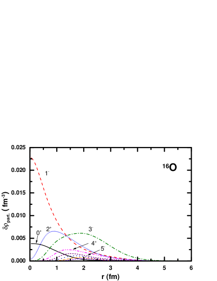
Figure 1: Contributions to $\delta\rho_{part.}$ of the $J^{\pi}$ multipoles from $0^{+}$ to $8^{+}$, in ¹⁶O. The unlabelled curves correspond to $J^{\pi}=6^{+},7^{-},8^{+}$.

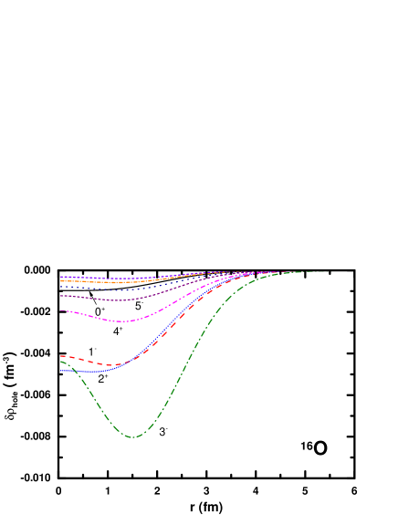
Figure 2: Same as Fig.1, for $\delta\rho_{hole}$ in ¹⁶O.

Summing over the partial contributions we obtain the corrections $\delta\rho_{part.}$, $\delta\rho_{hole}$ and $\delta\rho$ which are displayed in Fig.3. There are strong cancellations between $\delta\rho_{part.}$ and $\delta\rho_{hole}$, and the net result is small. We note that the analytical structure of Eqs.(12-13) insures that the integral of $\delta\rho$ over space is zero and hence, the total number of neutrons and protons is not affected by the RPA corrections. This is well verified in our numerical results.

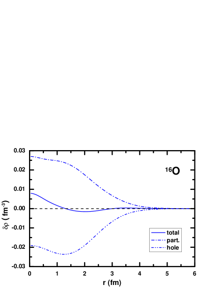
Figure 3: The summed corrections $\delta\rho_{part.}$, $\delta\rho_{hole}$ and their total $\delta\rho$ in ¹⁶O.

In Fig.4 are shown the mass and charge densities, both in the correlated (RPA) and uncorrelated (RMF) cases. For the charge density the effects of the center-of-mass motion and of the finite proton size are included by the usual folding procedure[14]. For the mass density $\delta\rho(r)$ the correlations tend to fill up the hole in the central region while the surface becomes slightly steeper. The same tendency appears in the charge density to a lesser extent. In the inset of Fig.4 the charge density is shown in logarithmic scale in order to display the differences in the tails in the asymptotic region beyond 6 fm. It is seen that the correlations induce in the outer region a tail which decreases less rapidly than the uncorrelated density. To have a more global measure of the changes caused by the RRPA correlations, the root mean square (rms) radii of the densities are shown in Table 1. The changes on radii appear to be modest, of the order of 0.7%-0.8%.

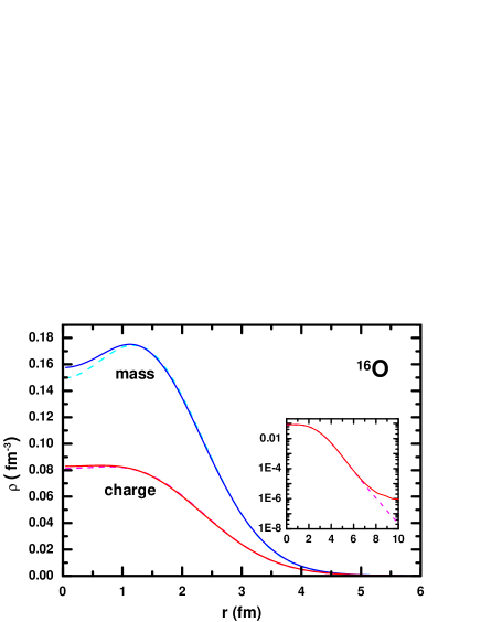
Figure 4: The uncorrelated (dashed lines) and correlated (solid lines) mass and charge densities in ¹⁶O. In the inset are shown the charge densities in log scale.

Table 1: Mass and charge rms radii in ¹⁶O and ⁴⁰Ca, calculated with uncorrelated RMF and correlated RPA densities. All units are in fm.

Nucleus		$\left<r^{2}_{\mbox{\scriptsize m}}\right>^{1/2}$	$\left<r^{2}_{\mbox{\scriptsize ch}}\right>^{1/2}$
16O	RMF	$2.594$	$2.729$
	RMF+RPA	$2.614$	$2.747$
40Ca	RMF	$3.346$	$3.466$
	RMF+RPA	$3.385$	$3.501$

4.2 DENSITIES OF ${}^{40}{\rm Ca}$

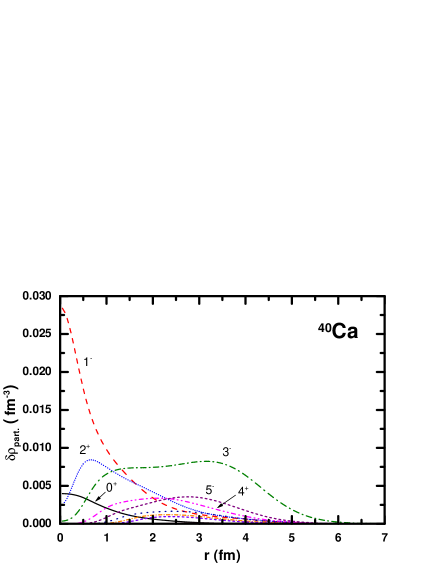
Figure 5: Contributions to $\delta\rho_{part.}$ of the $J^{\pi}$ multipoles from $0^{+}$ to $10^{+}$, in ⁴⁰Ca. The unlabelled curves correspond to $J^{\pi}=6^{+},7^{-},8^{+},9^{-},10^{+}$.

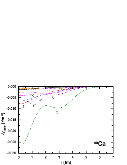
Figure 6: Same as Fig.5, for $\delta\rho_{hole}$ in ⁴⁰Ca.

In Figs.5-6 we present the respective contributions to $\delta\rho_{part.}$ and $\delta\rho_{hole}$ of the various multipolarities $J^{\pi}$ of the RPA states, in the nucleus ${}^{40}{\rm Ca}$. Here again, the dominant contributions come from the multipoles $1^{-},2^{+}$ and $3^{-}$, and the convergence is reached at $J^{\pi}=10^{+}$. It can be noted that the $1^{-}$ and $2^{+}$ contributions are localized near the nuclear center whereas the $3^{-}$ contributions extend over the nuclear volume. The summed corrections $\delta\rho_{part.}$, $\delta\rho_{hole}$ and $\delta\rho$ are displayed in Fig.7. The net effect on $\delta\rho$ is still small because of the cancellations between $\delta\rho_{part.}$ and $\delta\rho_{hole}$, but its shape is different from that of the ${}^{16}O$ case: the correction is negative from the center to about 3.5 fm, and positive afterwards since the number of particles must be conserved. Thus, the change on rms radii becomes slightly larger and of the order of 1%, as it can be seen in Table 1. The mass density and charge distribution (corrected for center of mass and finite proton size effects as in the case of ¹⁶O) are shown in Fig.8.

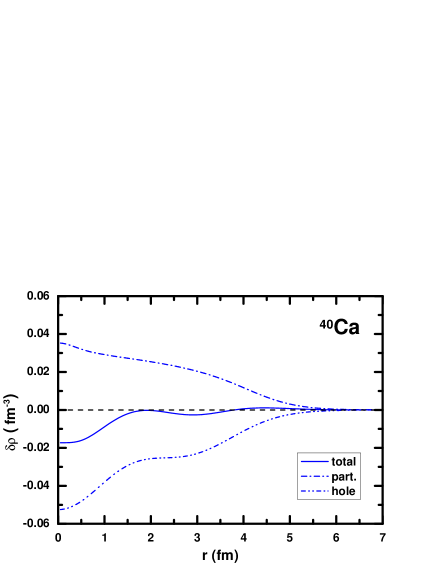
Figure 7: Same as Fig.3, for ⁴⁰Ca.

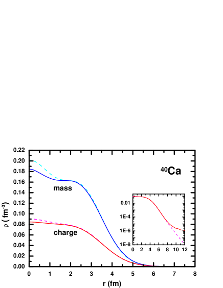
Figure 8: Same as Fig.4, for ⁴⁰Ca.

4.3 DENSITIES OF ${}^{48}{\rm Ca}$

For this nucleus with a sizable neutron excess we will examine separately the neutron and proton distributions and show that the long range correlations produce different effects on neutrons and on protons. In Fig.9 are shown the partial contributions of various multipoles to $\delta\rho_{part.}^{(\nu)}$ and $\delta\rho_{part.}^{(\pi)}$. It can be seen that the different multipoles contribute in a similar way to the neutron and proton densities. Again, the dominant multipoles are those below $J=4$ and the convergence is reached before $J=10$. The situation is slightly different for $\delta\rho_{hole}^{(\nu)}$ and $\delta\rho_{hole}^{(\pi)}$ as one can see in Fig.10. The most important difference between neutron and proton densities is seen in the contribution of the $J^{\pi}=3^{-}$ multipole. This can be understood by looking at the expression (15) for $\delta\rho_{hole}$. In the case of neutrons the important configurations $[(2s1/2,1d5/2,1d3/2)^{-1}(1f7/2)^{1}]_{3^{-}}$ are missing while they are allowed for protons. This results in an important contribution from $3^{-}$ states to the proton density between 0 and 2 fm, as compared to the neutron density.

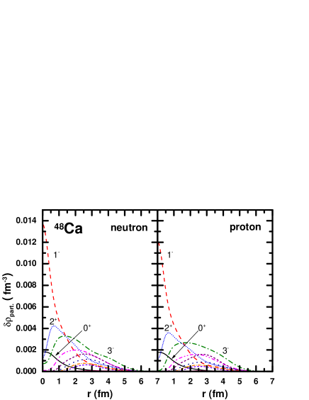
Figure 9: Contributions to $\delta\rho_{part.}^{(\nu)}$ (left panel) and to $\delta\rho_{part.}^{(\pi)}$ (right panel) of the $J^{\pi}$ multipoles from $0^{+}$ to $10^{+}$, in ⁴⁸Ca. The unlabelled curves correspond to $J^{\pi}=4^{+},5^{-},6^{+},7^{-},8^{+},9^{-},10^{+}$.

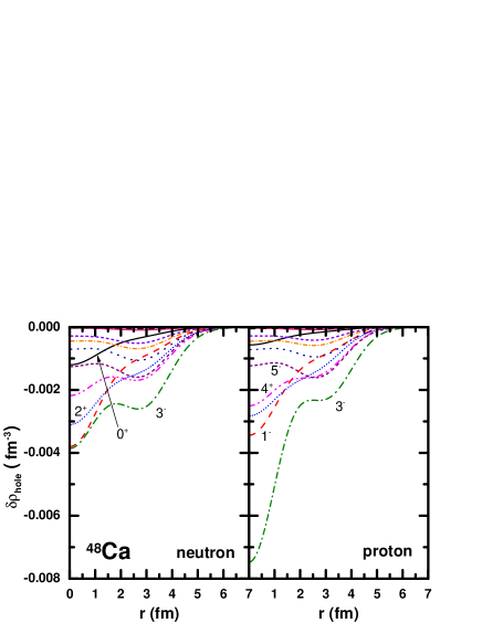
Figure 10: Same as Fig.9, for $\delta\rho_{hole}^{(\nu)}$ (left panel) and $\delta\rho_{hole}^{(\pi)}$ (right panel) in ⁴⁸Ca.

Summing up the contributions of various multipoles we obtain the density corrections $\delta\rho^{(\nu,\pi)}_{part.}$, $\delta\rho^{(\nu,\pi)}_{hole}$ and their sum $\delta\rho^{(\nu,\pi)}$. The results are shown in Fig.11 for neutrons and protons separately. One can notice that the signs of the corrections are opposite for neutrons and protons, in the central region up to 2 fm. The corrections become negative between 2.5 to 4 fm, and finally they are positive in the outer part. In Fig.12 we show the mass and charge densities of ⁴⁸Ca calculated with the uncorrelated (RMF) and correlated (RMF+RPA) ground states. The general effect of correlations is to lower down slightly the density near the center and to shift the corresponding particles to the outer region. The exponent of the exponential tail is changed somewhat beyond 8 fm. The values of rms radii for uncorrelated and correlated densities are summarized in Table 2. The changes in neutron and mass radii are relatively small (0.4% and 0.6%, respectively) whereas the changes of proton density radius (0.9%) and charge radius (0.8%) are more sizable.

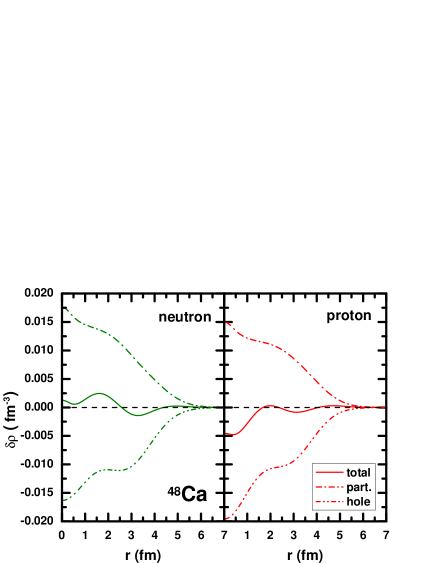
Figure 11: The corrections to neutron density (left panel) and proton density (right panel) in ⁴⁸Ca.

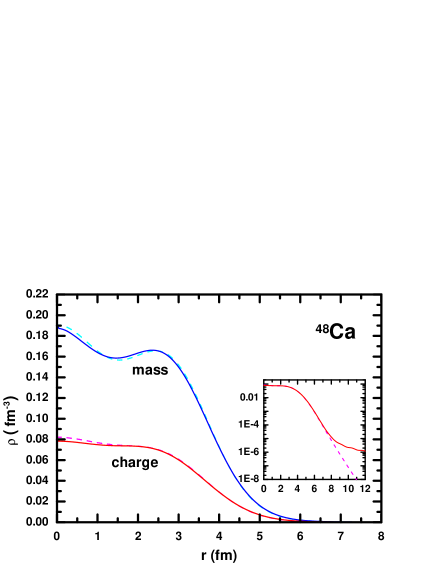
Figure 12: Same as Fig.4, for ⁴⁸Ca.

Table 2: Neutron, proton, mass and charge rms radii in ⁴⁸Ca, calculated with uncorrelated RMF and correlated RPA densities. All units are in fm.

Nucleus		$\left<r^{2}_{n}\right>^{1/2}$	$\left<r^{2}_{p}\right>^{1/2}$	$\left<r^{2}_{\mbox{\scriptsize m}}\right>^{1/2}$	$\left<r^{2}_{\mbox{\scriptsize ch}}\right>^{1/2}$
48Ca	RMF	$3.576$	$3.389$	$3.499$	$3.482$
	RMF+RPA	$3.592$	$3.420$	$3.521$	$3.511$

Finally, it is interesting to consider the respective roles of the Fermi and Dirac states in generating the corrections to the densities, in the case of RRPA correlations. In Fig.13 we show the separate contributions of the Fermi sector and Dirac sector to the density corrections $\delta\rho_{part.}$, $\delta\rho_{hole}$ and their sum $\delta\rho$. It can be seen that the contributions of the Fermi and Dirac sectors to $\delta\rho_{part.}$ are both positive whereas they are both negative for $\delta\rho_{hole}$. The magnitudes of Fermi and Dirac corrections are comparable. Thus, the Fermi and Dirac sectors play equally important roles in the density corrections. The fact that the total correction $\delta\rho$ remains small is due to the large cancellation between the positive $\delta\rho_{part.}$ and the negative $\delta\rho_{hole}$.

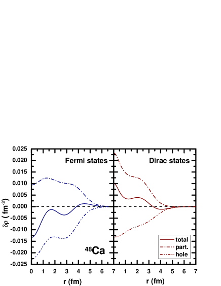
Figure 13: The contributions of Fermi states (left panel) and Dirac states (right panel) to the mass densities $\delta\rho_{part.}$, $\delta\rho_{hole}$ and $\delta\rho$ in ⁴⁸Ca.

5 CONCLUSION

In this work we have calculated the effects of RPA correlations on the ground state densities of some closed shell and closed subshell nuclei. This has been done for the relativistic mean field model and relativistic RPA theory, using a density-dependent effective Lagrangian with sigma, omega and rho couplings. We have stressed the peculiarity of the relativistic approach as compared to the usual non-relativistic approach, with the important effects coming from the negative energy (Dirac) sector. The presence of the Dirac states is inherent to the relativistic approach because one needs the completeness of the single-particle basis.

The long range correlation effects on densities are found to be limited although not negligible. It turns out that the main important multipolarities are the low $J$ modes, which is to be expected because the important collective excitations correspond to these low multipoles. The partial contributions to densities decrease rapidly with increasing $J$, and it is sufficient to drop the contributions beyond $J=8$ in ¹⁶O and $J=10$ in ^40,48Ca.

We have used in this work the DD-ME2 effective Lagrangian which gives a good description of nuclear ground states in the RMF approach, and it is working well for collective excitations of electric type, i.e., transitions of natural parity $\pi=(-1)^{J}$ described by RRPA without exchange terms[7]. However, it is not necessarily suitable for unnatural parity excitations, and this is the reason why we have not considered in this work the effects of magnetic transitions such as spin and spin-isospin modes. This must await future work where the effective Lagrangian is treated in Hartree+Fock approximation[15] and where the possibility to have pion- and $\rho$ tensor-coupling would enable one to describe on the same footing the electric and magnetic transitions.

Acknowledgements

This work is partly supported by the French CNRS program PICS (contract no. 3473), the European Community project Asia-Europe Link in Nuclear Physics and Astrophysics CN/Asia-Link 008 (94791), and the National Natural Science Foundation of China under Grant Numbers 10435010 and 10221003.

References

- [1] A.M. Lane, Nuclear Theory, Benjamin, New York, 1964.
- [2] D. Gogny, Lecture Notes in Physics, Springer, Berlin, 1979, p.88.
- [3] M. Dupuis, S. Karataglidis, E. Bauge, J.P. Delaroche, D. Gogny, Phys. Rev. C 73, 014605 (2006).
- [4] B.D. Serot, J.D. Walecka, Adv. Nucl. Phys. 16, 1 (1986).
- [5] P. Ring, Prog. Part. Nucl. Phys. 37, 193 (1996).
- [6] J. Meng, H. Toki, S.G. Zhou, S.Q. Zhang, W.H. Long, L.S. Geng, Prog. Part. Nucl. Phys. 57, 470 (2006).
- [7] T. Nikšić, D. Vretenar, P. Ring, Phys. Rev. C 66, 064302 (2002).
- [8] D. Vretenar, A.V. Afanasjev, G.A. Lalazissis, P. Ring, Phys. Rep. 409, 101 (2005).
- [9] G.A. Lalazissis, T. Nikšić, D. Vretenar, P. Ring, Phys. Rev. C 71, 024312 (2005).
- [10] P. Ring, Z.Y. Ma, N. Van Giai, D. Vretenar, A. Wandelt, L.G. Cao, Nucl. Phys. A694, 249 (2001).
- [11] P. Ring, P. Schuck, The Nuclear Many-Body Problem, Springer, New York, 1980.
- [12] D.J. Rowe, Phys. Rev. 175, 1283 (1968).
- [13] P.J. Ellis, Nucl. Phys. A 155, 625 (1970).
- [14] X. Campi, D.W. Sprung, Nucl. Phys. A 194, 401 (1972).
- [15] W.H. Long, N. Van Giai, J. Meng, Phys.Lett. B 640, 150 (2006).