EFT for DFT

These lectures give an overview of the ongoing application of effective field theory (EFT) and renormalization group (RG) concepts and methods to density functional theory (DFT), with special emphasis on the nuclear many-body problem. Many of the topics covered are still in their infancy, so rather than a complete review these lectures aim to provide an introduction to the developing literature.

1 EFT, RG, DFT for Fermion Many-body Systems

1.1 Overview of Fermion Many-Body Systems

There are a wide range of many-body systems featuring fermion degrees of freedom. These can be collections of “fundamental” fermions (electrons, quarks, …) or of composites each made of odd number of fermions (e.g., protons). Here are some general categories and examples:

1. Isolated atoms or molecules, which contain electrons interacting via the long-range (screened) Coulomb force.

2. Bulk solid-state materials, such as metals, insulators, semiconductors, superconductors, etc.

3. Liquid ³He (a superfluid!).

4. Cold fermionic atoms in (optical) traps (note that ⁶Li is a fermion but ⁷Li is a boson).

5. Atomic nuclei.

6. Neutron stars, which could mean neutron matter or color superconducting quark matter.

DFT has been most widely applied to systems in categories 1 and 2. We will focus in these lectures on categories 4 and 5 (and neutrons stars are treated in Thomas Schäfer’s lectures).

For our purposes, it won’t matter whether the fermions are structureless (as far as we know) such as quarks or electrons, or are composites such as interacting atoms. Note that an individual atom, studied as a many-body system of electrons (with external potential from the nucleus) is a fermion many-body system, while a collection of these atoms might be either a boson or fermion many-body system Fermions .

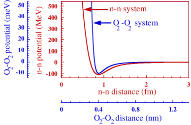
Figure 1: Molecule-molecule and nucleon-nucleon potentials compared Jacek .

If we label the axes appropriately in Fig. 1 (note the many orders of magnitude difference!), we see qualitative similarities between the central part of a conventional nucleon-nucleon (NN) potential and potentials between atoms or molecules (a Lennard-Jones potential is shown). In particular, there is midrange attraction and strong short-range repulsion (or a “hard core”). In the atomic case, the attraction is van der Waals in nature from induced polarization (which is why it falls off as $1/r^{6}$), and the rapid repulsion is from when the electron clouds overlap. In the nuclear case, the long- and mid-range attraction is mostly from one- and two-pion exchange. The hard core is often described in terms of vector-meson exchange but is generally phenomenological. The potential shown is the central part of the NN interaction; there are also important spin dependences and a non-central tensor force Preston75 .

What might one expect qualitatively from a many-body system with such a potential? Start with the equation of state of an ideal gas $PV=nRT$ ($n$ is number of moles). Hard-core means “excluded volume” so $V\rightarrow(V-nb)$ with $b$ constant. Attraction lowers the pressure on the container, so we find: $P=\frac{nRT}{V-nb}-\frac{an^{2}}{V^{2}}$. The end result is a van der Waals equation of state: $(P+\frac{an^{2}}{V^{2}})(V-nb)=nRT$, which has a liquid-gas phase transition. This is consistent with nuclei! The hard core keeps particles apart, leading to “short-range” correlations in the wave function. They make many-body problems difficult but might seem to be essential in saturating the nuclear liquid. Both liquid helium and nuclei can be thought of as liquid drops, whose radii scale with the number of particles $A$ to the 1/3 power: $R\sim r_{0}A^{1/3}$. If a hard core of radius $c$ is responsible for saturation, one can estimate that $0.55c\leq r_{0}\leq 2.4c$ JACKSON92 ; JACKSON94 . Liquid ³He has $r_{0}\sim 2.4\,\mbox{A}\sim c$, but for nuclei $r_{0}\sim 1.1\,\mbox{fm}\sim 2.75c$. This implies that nuclear matter is dilute and “delicately” bound, which means that an EFT expansion may be particularly useful. Other questions we might ask are whether there are common (“universal”) features of atomic and nuclear systems, and how to we relate the many-body physics to more fundamental underlying theories? As we’ll see, EFT will also help to address these questions.

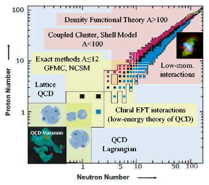
Figure 2: Overview of low-energy many-body nuclear systems Achim1 .

In Fig. 2, we show the “big picture” of low-energy nuclear physics, which features a specific scientific goal of predicting properties of unstable nuclei (the non-black squares), and a general scientific goal, which is connecting the whole picture from quantum chromodynamics (QCD) to superheavy nuclei in a systematic way with robust predictions. In principle, the nuclear part of the problem is simple: given internucleon potentials, just solve the many-body Schrödinger equation. This turns out to be feasible only for the smallest nuclei.

Why is this many-body problem so difficult computationally? Let’s think about the many-body Schrödinger wave function JoeC . How can we represent the wave function for an $A$-body nucleus? Consider a ⁸Be ($Z=4$ protons, $N=4$ neutrons) wave function with spin, isospin, and space components:

$$|\Psi\rangle=\sum_{\sigma,\tau}\chi_{\sigma}\chi_{\tau}\phi({\bf R})\;,\quad\mbox{where ${\bf R}$ are the $3A$ spatial coordinates}\;,$$

$$\chi_{\sigma}=\downarrow_{1}\uparrow_{2}\cdots\downarrow_{A}\ \mbox{($2^{A}$ terms)\ }{=256\ \mbox{for\ }A=8}\;,$$

$$\chi_{\tau}=n_{1}n_{2}\cdots p_{A}\ \mbox{($\frac{A!}{N!Z!}$ terms)\ }{=70\ \mbox{for\ }^{8}\mbox{Be}}\;.$$

So for ⁸Be there are 17,920 complex functions in $3A-3=21$ dimensions! Suppose for a nucleus of size 10 fm you represent this with a mesh spacing of 0.5 fm. You would need $10^{27}$ grid points! Obviously we need to drastically reduce the necessary degrees of freedom.

An extreme approximation to the full many-body wave function is the Hartree-Fock wave function, which is the best single Slater determinant in a variational sense:

$$|\Psi_{\rm HF}\rangle=\det\{\phi_{i}({\bf x}),i=1\cdots A\}\,,\quad{\bf x}=({\bf r},\sigma,\tau)\;.$$ (1)

The Hartree-Fock energy in the presence of an external potential is RINGSCHUCK

$$\langle\Psi_{\rm HF}|\widehat{H}|\Psi_{\rm HF}\rangle =$$ (2)

$$\sum_{i=1}^{A}\frac{\hbar^{2}}{2M}\int\!\!d{\bf x}\,\bm{\nabla}\phi^{\ast}_{i}\bm{\cdot}\bm{\nabla}\phi_{i}{+\frac{1}{2}\sum_{i,j=1}^{A}\int\!\!d{\bf x}\!\int\!\!d{\bf y}\,|\phi_{i}({\bf x})|^{2}v({\bf x},{\bf y})|\phi_{j}({\bf y})|^{2}}$$

$$\hbox{}{-\frac{1}{2}\sum_{i,j=1}^{A}\int\!\!d{\bf x}\!\int\!\!d{\bf y}\,\phi^{\ast}_{i}({\bf x})\phi_{i}({\bf y})v({\bf x},{\bf y})\phi^{\ast}_{j}({\bf y})\phi_{j}({\bf x})}$$

$$+\sum_{i=1}^{A}\int\!\!d{\bf y}\,v_{\rm ext}({\bf y})|\phi_{j}({\bf y})|^{2}\;.$$

We determine the $\phi_{i}$ by varying with fixed normalization:

$$\frac{\delta}{\delta\phi_{i}^{\ast}({\bf x})}\Bigl{(}\langle\Psi_{\rm HF}|\widehat{H}|\Psi_{\rm HF}\rangle-\sum_{j=1}^{A}\epsilon_{j}\int\!d{\bf y}\,|\phi_{j}({\bf y})|^{2}\Bigr{)}=0\;.$$ (3)

We solve this self-consistently, which is non-trivial because the potential is non-local, but drastically simpler than solving for the full wave function. However, while Hartree-Fock is a reasonable starting point for atoms, it is not for nuclear potentials of the form in Fig. 1 (e.g., note that the Argonne $v_{18}$ “1st order” curve in Fig. 5 is not even bound).

1.2 Density Functional Theory

An alternative to working with the many-body wave function is density functional theory (DFT) DREIZLER90 ; ARGAMAN00 ; fi03 , which as the name implies, has fermion densities as the fundamental “variables”. To date, the dominant application of DFT has been to the inhomogeneous electron gas, which means interacting point electrons in the static potentials of atomic nuclei. This has led to “ab initio” calculations of atoms, molecules, crystals, surfaces, and more caveat1 . DFT is founded on a theorem of Hohenberg and Kohn (HK): There exists an energy functional $E_{v_{\rm ext}}[\rho]$ of the density $\rho$ such that

$$E_{v_{\rm ext}}[\rho]=F_{\rm HK}[\rho]+\int\!d^{3}x\,v_{\rm ext}({\bf x})\rho({\bf x})\;,$$ (4)

where $F_{\rm HK}$ is universal (the same for any external potential $v_{\rm ext}$), the same for $H_{2}$ to DNA! This is useful if you can approximate the energy functional.

The general procedure is to introduce single-particle orbitals and to minimize the energy functional to obtain the ground-state energy $E_{gs}$ and density $\rho_{gs}$. This is called Kohn-Sham DFT, and is illustrated schematically in Fig. 3.

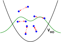
$\Longrightarrow$

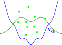
Figure 3: Kohn-Sham DFT for a $v_{\rm ext}=V_{\rm HO}$ harmonic trap. On the left is the interacting system and on the right the Kohn-Sham system. The density profile is the same in each.

Here the interacting density for $A$ fermions in the external potential $V_{\rm HO}$ is equal (by construction) to the non-interacting density in $V_{\rm KS}$. Orbitals $\{\psi_{i}({\bf x})\}$ in the local potential $V_{\rm KS}([\rho],{\bf x})$ are solutions to

$$[-\bm{\nabla}^{2}/2m+V_{\rm KS}({\bf x})]\psi_{i}=\varepsilon_{i}\psi_{i}$$ (5)

and determine the density

$$\rho({\bf x})=\sum_{i=1}^{A}|\psi_{i}({\bf x})|^{2}$$ (6)

(the sum is over the lowest $A$ states). The magical Kohn-Sham potential $V_{\rm KS}([\rho],{\bf x})$ is in turn determined from $\delta E_{v_{\rm ext}}[\rho]/\delta\rho({\bf x})$ (see below for an example). Thus the Kohn-Sham orbitals depend on the potential, which depends on the density, which depends on the orbitals, so we must solve self-consistently (for example, by iterating until convergence).

DFT for solid-state or molecular systems starts with the HK free energy for an inhomogeneous electron gas ARGAMAN00 :

$$F_{{\rm HK}}[\rho({\mathbf{x}})]=T_{{\rm KS}}[\rho({\mathbf{x}})]+\frac{e^{2}}{2}\!\int\!d^{3}x\,d^{3}x^{\prime}\frac{\rho({\mathbf{x}})\rho({\mathbf{x}^{\prime}})}{|{\bf x}-{\bf x^{\prime}}|}+E_{{\rm xc}}[\rho({\mathbf{x}})]\;.$$ (7)

Then $V_{\rm KS}=v_{\rm ext}-e\phi+v_{\rm xc}$ with $v_{\rm xc}({\mathbf{x}})=\delta E_{\rm xc}/\delta\rho({\mathbf{x}})$. To calculate the Kohn-Sham kinetic energy ${T_{{\rm KS}}[\rho({\mathbf{x}})]}$, find the normalized $\{\psi_{i},\epsilon_{i}\}$ from

$$\Bigl{(}-\frac{\hbar^{2}}{2m}\nabla^{2}+V_{\rm KS}({\mathbf{x}})\Bigr{)}\psi_{i}({\mathbf{x}})=\epsilon_{i}\psi_{i}({\mathbf{x}})$$ (8)

and, with $\rho({\mathbf{x}})=\sum_{i=1}^{A}|\psi_{i}({\mathbf{x}})|^{2}$,

$$T_{{\rm KS}}[\rho({\mathbf{x}})]=\sum_{i=1}^{A}\langle\psi_{i}|-\frac{\hbar^{2}}{2m}\nabla_{i}^{2}|\psi_{i}\rangle=\sum_{i=1}^{A}\epsilon_{i}-\int\!d^{3}x\,\rho({\mathbf{x}})V_{\rm KS}({\mathbf{x}})\;.$$ (9)

In practice, the DFT is usually based on the local density approximation (LDA): $E_{{\rm xc}}[\rho({\mathbf{x}})]\approx\int\!d^{3}x\,{\cal E}_{{\rm xc}}(\rho({\mathbf{x}}))$ with ${\cal E}_{{\rm xc}}(\rho)$ fit to a Monte Carlo calculation of the uniform electron gas. For example, one parametric formula for the energy density is ARGAMAN00

$${\cal E}_{\rm xc}(\rho)/\rho=-0.458/r_{s}-0.0666G(r_{s}/11.4)\;,$$ (10)

with

$$G(x)=\frac{1}{2}\left\{(1+x)^{3}\log(1+x^{-1})-x^{2}+\frac{1}{2}x-\frac{1}{3}\right\}\;.$$ (11)

This is just like a simple Hartree approach with the additional potential:

$$v_{\rm xc}({\bf x})=\left.\frac{d[{\cal E}_{\rm xc}(\rho)]}{d\rho}\right|_{\rho=\rho({\mathbf{x}})}\;.$$ (12)

The LDA is improved with the Generalized Gradient Approximation (GGA), such as the van Leeuwen–Baerends GGA ARGAMAN00 ,

$$v_{\rm xc}({\bf r})=-\beta\rho^{1/3}({\bf r})\frac{x^{2}({\bf r})}{1+3\beta x({\bf r})\sinh^{-1}(x({\bf r}))}$$ (13)

with $x=|\nabla\rho|/\rho^{4/3}$. For these Coulomb systems, Hartree-Fock is generally a good starting point, DFT/LDA is better, and DFT/GGA is better still.

There are some concerns, however, about DFT. Here are some quotes from the DFT literature that help motivate the application of EFT to DFT:

From A Chemist’s Guide to DFT KOCH2000 : “To many, the success of DFT appeared somewhat miraculous, and maybe even unjust and unjustified. Unjust in view of the easy achievement of accuracy that was so hard to come by in the wave function based methods. And unjustified it appeared to those who doubted the soundness of the theoretical foundations. ”

From Density Functional Theory ARGAMAN00 : “It is important to stress that all practical applications of DFT rest on essentially uncontrolled approximations, such as the LDA …”

From Meta-Generalized Gradient Approximation PERDEW99 “Some say that ‘there is no systematic way to construct density functional approximations.’ But there are more or less systematic ways, and the approach taken …here is one of the former.”

Thus, a microscopic, controlled, and systematic approach to DFT would be welcome.

We end this section with a preview of DFT as an effective action Polonyi2001 . Recall ordinary thermodynamics with $N$ particles at $T=0$. The thermodynamic potential is related to the partition function, with the chemical potential $\mu$ acting as a source to change $N=\langle\widehat{N}\rangle$,

$$\Omega(\mu)=-kT\ln Z(\mu)\qquad\mbox{and}\qquad N=-\left(\frac{\partial\Omega}{\partial\mu}\right)_{TV}\;.$$ (14)

If we invert to find $\mu(N)$ and apply a Legendre transform, we obtain

$$F(N)=\Omega(\mu(N))+\mu(N)N\;.$$ (15)

This is our (free) energy function of the particle number, which is analogous to the DFT energy functional of the density. Indeed, if we generalize to a spatially dependent chemical potential $J({\bf x})$, then

$$Z(\mu)\longrightarrow Z[J({\bf x})]\qquad\mbox{and}\qquad\mu N=\mu\int\psi^{\dagger}\psi\longrightarrow\int J({\bf x})\psi^{\dagger}\psi({\bf x})\;.$$ (16)

Now Legendre transform from $\ln Z[J({\bf x})]$ to $\Gamma[\rho({\bf x})]$, where $\rho=\langle\psi^{\dagger}\psi\rangle_{J}$, and we have DFT with $\Gamma$ simply proportional to the energy functional!

1.3 DFT for Nuclei: EFT and RG Approaches

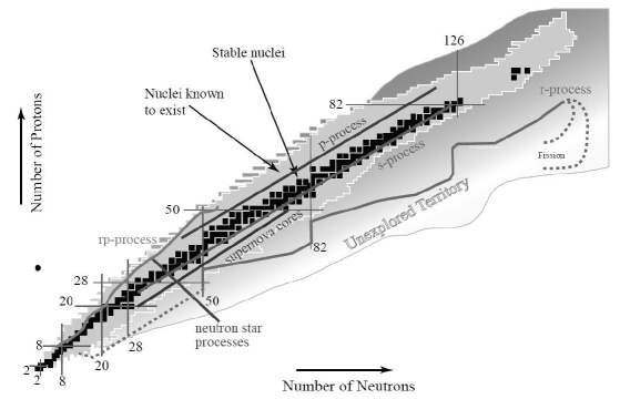
Figure 4: Table of the nuclides.

Figure 4 shows the table of the nuclides, labeled by the total numbers of protons and neutrons. For example, ²⁰⁸Pb is found at the intersection of the horizontal line labeled “82” (protons) and the vertical line labeled “126” (neutrons). Stable nuclei are in black, known in pink. Here are some basic nuclear physics questions (which everyone should know how to answer):

• Why is the slope of the black region less than a 45 degree angle once it is past $Z=N=20$ or so?

• How do the binding energies of the nuclei in black compare? (E.g., do they vary over a wide range? Do they have a regular pattern?)

• What happens to the binding energy as you move perpendicular to the black line?

• What is the difference between being unstable and unbound? What are the drip lines?

(See Preston75 ; RINGSCHUCK for nuclear physics background.) The nucleosynthesis r-process lives largely in “Unexplored Territory.” Radioactive beam facilities (existing and proposed) address this physics, as well as exotic nuclei such as halo nuclei and many other phenomena. As one gets further from stability, the importance of pairing grows, which highlights a difference between nuclear many-body physics and the physics of Coulomb systems, like atoms and molecules.

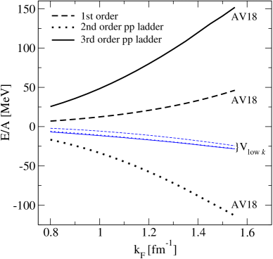
Figure 5: Nuclear matter in perturbation theory for a conventional NN potential (Argonne $v_{18}$) and a low-momentum potential Bogner_nucmatt .

Let’s try solving nuclear matter in low-order perturbation theory. One expects a minimum in the energy/particle ($E/A$) versus density (here the Fermi momentum $k_{\rm F}\propto\rho^{1/3}$) at about $k_{\rm F}\sim 1.35\,\mbox{fm}^{-1}$ and $E/A\sim-16\,$MeV. The standard Argonne $v_{18}$ potential AV18 is used in Fig. 5, with “Brueckner ladder” contributions shown order-by-order. First order is Hartree-Fock and it is not even bound! The repulsive core means that the series diverges badly.

But there is an energy density functional approach that seems to be based on Hartree-Fock (HF), which works quite well throughout Fig. 4. This is the phenomenological Skyrme HF approach RINGSCHUCK ; VB72 ; Dobaczewski:2001ed ; BENDER2003 . Recall from our earlier Hartree-Fock discussion that solving self-consistently is somewhat tricky because the potential is non-local. It would be much simpler if $v({\bf x},{\bf y})\propto\delta({\bf x}-{\bf y})$. This is the case with the Skyrme interaction $V_{2}^{\rm Skyrme}+V_{3}^{\rm Skyrme}$, where $\langle{\bf k}|V_{2}^{\rm Skyrme}|{\bf k^{\prime}}\rangle=t_{0}+\frac{1}{2}t_{1}({\bf k}^{2}+{\bf k^{\prime}}^{2})+t_{2}{\bf k}\cdot{\bf k^{\prime}}+iW_{0}(\mathbf{\sigma}_{1}+\mathbf{\sigma}_{2})\cdot{\bf k}\times{\bf k^{\prime}}$. This motivates the Skyrme energy density functional (for $N=Z$) RINGSCHUCK :

$${\cal E}[{\rho},{\tau},{\bf J}] \!\!=\!\! {1\over 2M}{\tau}+{3\over 8}t_{0}{\rho^{2}}+{1\over 16}t_{3}{\rho^{2+\alpha}}+{1\over 16}(3t_{1}+5t_{2}){\rho}{\tau}$$ (17)

$$\hbox{}+{1\over 64}(9t_{1}-5t_{2}){(\nabla\rho)^{2}}-{3\over 4}W_{0}{\rho}\nabla\cdot{\bf J}+{1\over 32}(t_{1}-t_{2}){\bf J}^{2}\;,$$

where ${\rho({\bf x})=\sum_{i}|\phi_{i}({\bf x})|^{2}}$ and ${\tau({\bf x})=\sum_{i}|\nabla\phi_{i}({\bf x})|^{2}}$ (see RINGSCHUCK for the ${\bf J}({\bf x})$ formula). We minimize $E=\int\!d{\bf x}\,{\cal E}[\rho,\tau,{\bf J}]$ by varying the (normalized) $\phi_{i}$’s,

$$\Bigl{(}-\mathbf{\nabla}{\frac{1}{2M^{*}({\bf x})}}\mathbf{\nabla}+{U({\bf x})}+\frac{3}{4}W_{0}\mathbf{\nabla}\rho\cdot\frac{1}{i}\mathbf{\nabla}\times\bf{\sigma}\Bigr{)}\,\phi_{i}({\bf x})=\epsilon_{i}\,\phi_{i}({\bf x})\;,$$ (18)

with $U=\frac{3}{4}t_{0}\rho+(\frac{3}{16}t_{1}+\frac{5}{16}t_{2})\tau+\cdots$ and $\frac{1}{2M^{*}({\bf x})}=\frac{1}{2M}+({3\over{16}}t_{1}+{5\over{16}}t_{2})\rho$. One iterates until the $\phi_{i}$’s and $\epsilon_{i}$’s are self-consistent.

While phenomenologically successful, there are many questions and possible criticisms of Skyrme HF. Typical [e.g., SkIII] model parameters are: $t_{0}=-1129$, $t_{1}=395$, $t_{2}=-95$, $t_{3}=14000$, $W_{0}=120$ (in units of MeV-fmⁿ). These seem large; is there an expansion parameter? Where does $\rho^{2+\alpha}$ come from? Why not $\rho^{2+\beta}$? Is this just parameter fitting? A famous quote from von Neumann (via Fermi via Dyson) says: “With four parameters I can fit an elephant, and with five I can make him wiggle his trunk.” One might also say that Skyrme HF is only a mean-field model, which is too simple to accommodate NN correlations. How do we improve the approach? Is pairing treated correctly? How does Skyrme HF relate to NN (and NNN) forces? And so on. There is also the observation that Skyrme functionals works well where there is already data, but elsewhere fails to give consistent predictions (and the theoretical error bar is unknown).

Rather than focus on the Skyrme interaction, we consider the Skyrme energy functional as an approximate DFT functional. (Note: this is the viewpoint of modern practitioners.) Our master plan is to use EFT and renormalization group (RG) methods to elevate something close to Skyrme HF to a full DFT treatment. We want to use EFT and RG to provide a systematic input potential, including three-body potentials, and to generate systematically improved energy functionals. At the same time, we want to be able to estimate theoretical errors, so that extrapolation is under control.

Table 1: (Nuclear) Many-Body Physics: “Old” Approach

One Hamiltonian for all problems and energy/length scales (not QCD!)	For nuclear structure, protons and neutrons with a local potential Table1 fit to NN data
Find the “best” potential	NN potential with $\chi^{2}/\mbox{dof}\approx 1$ up to $\sim 300\,$MeV energy Table2
Two-body data may be sufficient; many-body forces as last resort	Let phenomenology dictate whether three-body forces are needed (answer: yes! Table3 )
Avoid (hide) divergences	Add “form factor” to suppress high-energy intermediate states; don’t consider cutoff dependence Table4
Choose approximations by “art”	Use physical arguments (often handwaving) to justify the subset of diagrams used Table5

This is a relatively new and different approach. In Table 1 we summarize aspects of the “traditional” approach to the (nuclear) many-body problem that are being challenged by the EFT approach. There are many continuing successes of conventional many-body approaches. The idea is not to prove standard methods wrong but to highlight where new insight can be provided. For each “old” item in this table (see endnotes for further explanations), we’ll have a “new” perspective from EFT (see Table 2).

1.4 EFT Analogies

From an effective field theory we desire systematic calculations with error estimates. We want them to be robust and model independent, which will enable reliable extrapolation. To help understand how this is accomplished, we can explore useful analogies between EFT and sophisticated numerical analysis.

• Naive error analysis: pick a method and reduce the mesh size (e.g., increase grid points) until the error is “acceptable”. Sophisticated error analysis: understand scaling and sources of error (e.g., algorithm vs. round-off errors). Does it work as well as it should?

• Representation dependence means that not all ways of calculating are equally effective!

• Reliable extrapolation requires completeness of an expansion basis. An EFT lagrangian provides the analog of a complete basis.

Note: quantum mechanics makes EFT trickier than “classical” numerical analysis (see Lepage’s lectures)!

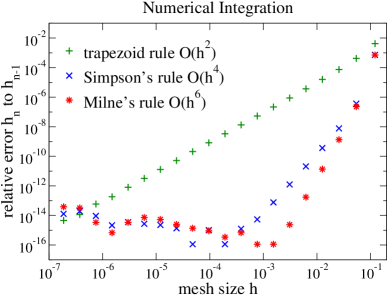
Figure 6: Error plots in numerical integration.

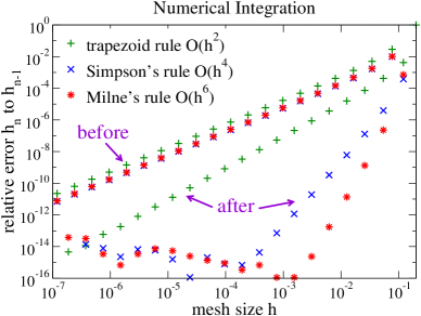
Figure 7: The representation can make a difference: errors for (19) vs. (20).

Consider the numerical calculation of an integral using equal-spaced integration rules of increasing sophistication. How do the numerical errors behave? Log-log plots of the relative error against a parameter such as the mesh size are very helpful; a straight line indicates a power law and the exponent is read off from the slope. An example is shown in Fig. 6. Similar plots can be made for order-by-order EFT calculations, as described in Peter Lepage’s lectures. Just like computer math is not equivalent to ordinary math, EFT is not the same as a theory applicable at all energies. It breaks down at high resolution, as the numerical calculations break down and degrade because of round-off errors at small mesh sizes. (Note: Don’t carry this analogy to extremes!) Next consider an elliptic integral:

$$\int_{0}^{1}\!\sqrt{(1-x^{2})(2-x)}\,dx$$ (19)

with errors plotted in Fig. 7. Something is wrong; the errors do not behave as expected. However, after a simple transformation:

$$\int_{0}^{\pi/2}\!\sin^{2}y\,\sqrt{2-\cos y}\,dy\;.$$ (20)

As seen in Fig. 7, the transformation makes a big difference! If you have freedom to change the representation, you can make a big difference in the ability to calculate accurately and easily. This is a moral we will apply when using EFT and RG methods to many-body problems.

1.5 Principles of Effective Low-Energy Theories

There are some basic physics principles underlying any low-energy effective model or theory. A high-energy, short-wavelength probe sees detail down to scales comparable to the wavelength. Thus, high-energy electron scattering at Jefferson Lab resolves the quark substructure of protons and neutrons in a nucleus. But at lower energies, details are not resolved, and one can replace short-distance structure with something simpler, as in a multipole expansion of a complicated charge or current distribution. So it is not necessary to do full QCD to do strong interaction physics at low energies, we can replace quarks and gluons by neutrons and protons (and pions). Chiral effective field theory is a systematic approach to carrying out this program using a local lagrangian framework.

It is not obvious that working at low resolution will work in quantum mechanics as it does for pixels or point dots or the classical multipole expansion, because virtual states can have high energies that are not, in reality, simple. But renormalization theory says it can be done! (See Lepage’s lectures and LEPAGEren ; Lepage .) Note that this doesn’t mean that we are insensitive to all short-distance details, only that their effects at low energies can be accounted for in a simple way.

We can use the possibility of changing the resolution scale to change the “perturbativeness” of nuclei. There are several sources of nonperturbative physics for nucleon-nucleon interactions:

1. Strong short-range repulsion (“hard core”).

2. Iterated tensor ($S_{12}$) interactions (e.g., from pion exchange).

3. Near zero-energy bound states.

In Coulomb DFT, Hartree-Fock gives the dominate contribution to the energy, and correlations are small corrections. This may be why DFT works. In contrast, for NN interactions, correlations $\gg$ HF; does this mean DFT fails?? However, the first two sources depend on the resolution (i.e., the cutoff of high-energy physics), and the third one is affected by Pauli blocking. Thus we might use the freedom of low-energy theories to simplify calculations.

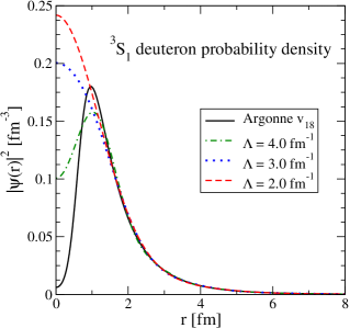
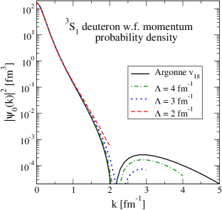
Figure 8: The deuteron probability density at different resolutions (as indicated by the sharp momentum cutoff $\Lambda$).

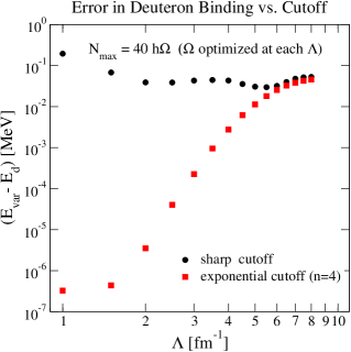
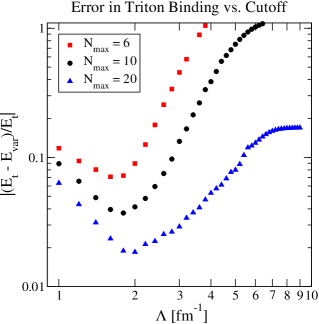
Figure 9: Variational calculations at different resolutions Bogner:2005fn ; Bogner:2006a .

We can see the impact of different resolutions on the deuteron wave function in Fig. 8. The repulsive core leads to short-distance suppression and important high-momentum (small $\lambda$) components. This makes the many-body problem complicated. In contrast, potentials evolved by renormalization group (RG) methods to low momentum, generically called $V_{{\rm low\,}k}$ Vlowk1 ; Vlowk2 ; VlowkRG , have much simpler wave functions! (See Andreas Nogga’s lectures for more detail on such potentials.) We note that chiral EFT potentials are naturally low-momentum potentials, but lowering their cutoffs further is generally advantageous. The consequence of lower resolution for variational calculations is illustrated in Fig. 9 Bogner:2005fn ; Bogner:2006a . Note that the improvement for the deuteron comes with smooth (exponential) cutoffs Bogner:2006tw , which is another example of how the representation can make a difference.

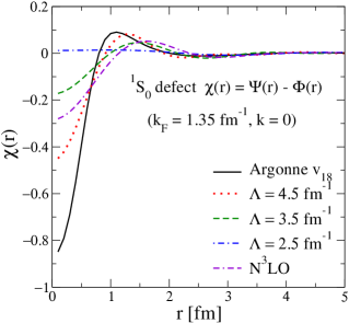
Figure 10: Two-body correlations in nuclear matter.

These observations carry over to nuclear matter as well, as seen in Fig. 10 (although the effect with lowered cutoff in the important ³S₁ channel is less dramatic). In medium, the phase space in the pp-channel is strongly suppressed:

$$\int_{k_{\rm F}}^{{\infty}}q^{2}\,dq\frac{V_{NN}(k^{\prime},q)V_{NN}(q,k)}{k^{2}-q^{2}}$$ (21)

compared to

$$\int_{k_{\rm F}}^{{\Lambda}}q^{2}\,dq\frac{V_{{\rm low\,}k}(k^{\prime},q)V_{{\rm low\,}k}(q,k)}{k^{2}-q^{2}}\;.$$ (22)

(In addition, the potential itself gets smaller in magnitude in the integration region.) This tames the hard core, tensor force, and the bound state. If we return to Fig. 5, we see the consequence, which is very rapid convergence (by 2nd order) of the in-medium T-matrix for $V_{{\rm low\,}k}$ Bogner_nucmatt . But there is no saturation in sight!

There were active attempts to transform away hard cores and soften the tensor interaction in the late sixties and early seventies KERMAN66 ; KERMAN67 ; KERMAN73 . But the requiem for soft potentials was given by Bethe (1971):

“Very soft potentials must be excluded because they do not give saturation; they give too much binding and too high density. In particular, a substantial tensor force is required.”

The next 30+ years were spent trying to solve accurately with “hard” potentials. But the story is not complete: three-nucleon forces (3NF)! When they are added consistently, we have the advantages of soft potentials while answering Bethe’s criticism.

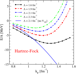
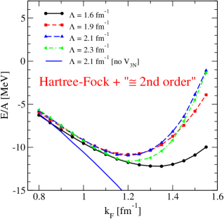
Figure 11: Nuclear matter energy per particle Bogner_nucmatt .

Ideally we would start with chiral NN + 3NF EFT interactions and then evolve downward in $\Lambda$. What is possible now is to run the NN and fit 3NF EFT at each $\Lambda$ Vlowk3N . The consequence is shown in Fig. 11. There is saturation even at the Hartree-Fock level, which is now driven by the three-body force. At second order, the cutoff dependence is greatly reduced and the minimum moves closer to the empirical point. One might worry that the three-body force is unnaturally large, but it is consistent with EFT power counting. Excellent results are also found for neutron matter. While there is much to be done, these results are very encouraging and motivate a microscopic DFT for nuclei.

1.6 Summary

In summary, there is a new attitude for many-body physics inspired by effective field theory. Bethe wrote about the nuclear case:

“The theory must be such that it can deal with any nucleon-nucleon (NN) force, including hard or ‘soft’ core, tensor forces, and other complications. It ought not to be necessary to tailor the NN force for the sake of making the computation of nuclear matter (or finite nuclei) easier, but the force should be chosen on the basis of NN experiments (and possibly subsidiary experimental evidence, like the binding energy of H³).”

The new attitude is to instead seek to make the problem easier. It’s like the old vaudeville joke about a doctor and his patient:
Patient: Doctor, doctor, it hurts when I do this!
Doctor: Then don’t do that.
We also follow Weinberg’s Third Law of Progress in Theoretical Physics: “You may use any degrees of freedom you like to describe a physical system, but if you use the wrong ones, you’ll be sorry!” We conclude with a new table (Table 2) of many-body physics, contrasting the old and the new approaches.

Table 2: (Nuclear) Many-Body Physics: “Old” vs. “New”

One Hamiltonian for all problems and energy/length scales	Infinite # of low-energy potentials; different resolutions $\Longrightarrow$different dof’s and Hamiltonians
Find the “best” potential	There is no best potential $\Longrightarrow$use a convenient one!
Two-body data may be sufficient; many-body forces as last resort	Many-body data needed and many-body forces inevitable
Avoid divergences	Exploit divergences (cutoff dependence as tool)
Choose diagrams by “art”	Power counting determines diagrams and truncation error

2 EFT/DFT for Dilute Fermi Systems

2.1 Thermodynamics Interpretation of DFT

As an analogy, consider a system of spins $S_{i}$ on a lattice with interaction strength $g$ NEGELE88 . The partition function has all the information about the energy and magnetization of the system:

$${\cal Z}={\rm Tr\,}e^{-\beta g\sum_{\{i,j\}}S_{i}S_{j}}\;.$$ (23)

The magnetization $M$ is

$$M \!\!=\!\! \Bigl{\langle}\sum_{i}S_{i}\Bigr{\rangle}$$ (24)

$$\!\!=\!\! \frac{1}{\cal Z}\,{\rm Tr\,}\biggl{[}\Bigl{(}\sum_{i}S_{i}\Bigr{)}e^{-\beta g\sum_{\{i,j\}}S_{i}S_{j}}\biggr{]}\;.$$ (25)

Now add an external magnetic probe source $H$. The source adjusts the spin configurations near the ground state,

$${\cal Z}[H]=e^{-\beta F[H]}={\rm Tr\,}e^{-\beta(g\sum_{\{i,j\}}S_{i}S_{j}{-H\sum_{i}S_{i}})}\;.$$ (26)

Variations of the source yield the magnetization

$$M=\Bigl{\langle}\sum_{i}S_{i}\Bigr{\rangle}_{H}=-\frac{\partial F[H]}{\partial H}\;,$$ (27)

where $F[H]$ is the Helmholtz free energy. For the ground state, we set $H=0$ (or equal to a real external source) at the end.

Now if we find $H[M]$ by inverting $M[H]$,

$$M=\Bigl{\langle}\sum_{i}S_{i}\Bigr{\rangle}_{H}=-\frac{\partial F[H]}{\partial H}\;,$$ (28)

we can Legendre transform to the Gibbs free energy

$$\Gamma[M]=F[H]+H\,M\;.$$ (29)

Then the ground-state magnetization $M_{\rm gs}$ follows by minimizing $\Gamma[M]$:

$$H=\frac{\partial\Gamma[M]}{\partial M}\longrightarrow\left.\frac{\partial\Gamma[M]}{\partial M}\right|_{M_{\rm gs}}=0\;.$$ (30)

Thus, we have a function of $M$ (or functional if $H$ is inhomogeneous) that is minimized at the ground-state free energy and magnetization.

DFT has an analogous structure as an effective action Polonyi2001 . An effective action is generically the Legendre transform of a generating functional with an external source (or sources). For DFT, we use a source to adjust the density instead of the magnetization. The partition function in the presence of $J(x)$ coupled to the density is (we’ll use a schematic notation here):

$${\cal Z}[J]=e^{-W[J]}\sim{\rm Tr\,}e^{-\beta({\widehat{H}}+J\,\widehat{\rho})}\longrightarrow\int\!{\cal D}[\psi^{\dagger}]{\cal D}[\psi]\,e^{-\int[{\cal L}+J\,\psi^{\dagger}\psi]}\;.$$ (31)

The density $\rho(x)$ in the presence of $J(x)$ is (keep in mind that we want $J=0$ eventually),

$$\rho(x)\equiv\langle\widehat{\rho}(x)\rangle_{J}=\frac{\delta W[J]}{\delta J(x)}\;.$$ (32)

After inverting to find $J[\rho]$, we Legendre transform from $J$ to $\rho$:

$$\Gamma[\rho]=W[J]-\int\!J\,\rho\quad\mbox{and}\quad J(x)=-\frac{\delta\Gamma[\rho]}{\delta\rho(x)}\;.$$ (33)

Now consider the partition function in the zero-temperature limit of a Hamiltonian with time-independent source $J({\bf x})$ ZINNJUSTIN ; Minkowski :

$${{\widehat{H}}}(J)={{\widehat{H}}}+\int\!J\,\psi^{\dagger}\psi\;.$$ (34)

If the ground state is isolated (and bounded from below),

$$e^{-\beta{\widehat{H}}}=e^{-\beta E_{0}}\left[|0\rangle\langle 0|+{\cal O}\bigl{(}e^{-\beta(E_{1}-E_{0})}\bigr{)}\right]\;.$$ (35)

As $\beta\rightarrow\infty$, ${\cal Z}[J]$ yields the ground state of ${{\widehat{H}}}(J)$ with energy $E_{0}(J)$:

$${E_{0}(J)}=\lim_{\beta\rightarrow\infty}-\frac{1}{\beta}\log{\cal Z}[J]=\frac{1}{\beta}W[J]\;.$$ (36)

Substitute and separate out the pieces:

$$E_{0}(J)=\langle{{\widehat{H}}}(J)\rangle_{J}=\langle{\widehat{H}}\rangle_{J}+\int\!J\langle\psi^{\dagger}\psi\rangle_{J}=\langle{{\widehat{H}}}\rangle_{J}+\int\!J\,\rho(J)\;.$$ (37)

Rearranging, the expectation value of ${{\widehat{H}}}$ in the ground state generated by $J[\rho]$ is

$${\langle{{\widehat{H}}}\rangle_{J}}=E_{0}(J)-\int J\,\rho=\frac{1}{\beta}\Gamma[\rho]\;.$$ (38)

Let’s put it all together:

$$\frac{1}{\beta}\Gamma[\rho]=\langle{{\widehat{H}}}\rangle_{J}\stackrel{{\scriptstyle J\rightarrow 0}}{{\longrightarrow}}E_{0}\quad\mbox{and}\quad J(x)=-\frac{\delta\Gamma[\rho]}{\delta\rho(x)}\stackrel{{\scriptstyle J\rightarrow 0}}{{\longrightarrow}}{\left.\frac{\delta\Gamma[\rho]}{\delta\rho(x)}\right|_{\rho_{\rm gs}({\bf x})}=0}\;.$$ (39)

So for static $\rho({\bf x})$, $\Gamma[\rho]$ is proportional to the DFT energy functional $F_{\rm HK}$! Furthermore, the true ground state (with $J=0$) is a variational minimum, so additional sources should be better than just one source coupling to the density (as we’ll consider below). The simple, universal dependence on external potential follows directly in this formalism:

$$\Gamma_{v}[\rho]=W_{v}[J]-\int\!J\,\rho=W_{v=0}[J+v]-\int\![(J+v)-v]\,\rho=\Gamma_{v=0}[\rho]+\int\!v\,\rho\;.$$ (40)

[Note: the functionals will change with resolution or field redefinitions; only stationary points are observables.]

There are a number of paths to the DFT effective action:

1. Follow the usual Coulomb Kohn-Sham DFT by calculating the uniform system as function of density, which yields an LDA (“local density approximation”) functional and a standard Kohn-Sham procedure. Improve the functional with a semi-empirical gradient expansion.

2. Derive the functional with an RG approach Schwenk:2004hm .

3. Use the auxiliary field method NAGAOSA ; STONE . Couple $\psi^{\dagger}\psi$ to an auxiliary field $\varphi$, and eliminate all or part of $(\psi^{\dagger}\psi)^{2}$. Add a source term $J\varphi$ and perform a loop expansion about the expectation value $\phi=\langle\varphi\rangle$. A Kohn-Sham version uses the freedom of the expansion to require the density be unchanged at each order.

4. The inversion method Fukuda:im ; VALIEV97 ; VALIEV ; RASAMNY98 yields a systematic Kohn-Sham DFT, based on an order-by-order expansion. For example, we can apply the EFT power counting for a dilute system.

We’ll expand here on the last path.

2.2 EFT for Dilute Fermi Systems

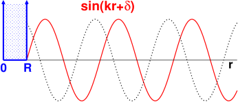
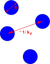
Figure 12: Hard-sphere phase shifts and scales at finite density.

We consider first one of the simplest many-body systems: a collection of “hard spheres,” which means that the potential is infinitely repulsive at a separation $R$ of the fermions. Since the potential is zero outside of $R$ and the wave function must vanish in the interior of the potential (so that the energy is finite), we can trivially write down the $S$-wave scattering solution for momentum $k$: it is just a sine function shifted by $kR$ from the origin (see Fig. 12). Our problem will be to find the energy per particle (and other observables) of a system of particles interacting with this potential at $T=0$, given the density.

Let’s do a quick review of scattering. (More details on scattering at this level can be found in practically any first-year graduate quantum mechanics text. For a more specialized but very readable account of nonrelativistic scattering, check out “Scattering Theory” by Taylor.) Consider relative motion with total momentum $P=0$:

$$\psi(r)\stackrel{{\scriptstyle r\rightarrow\infty}}{{\longrightarrow}}e^{i{\bf k\cdot r}}+{f(k,\theta)}\frac{e^{ikr}}{r}\;,$$ (41)

where $k^{2}={k^{\prime}}^{2}=ME_{k}$ and $\cos\theta=\hat{k}\cdot\hat{k}^{\prime}$. The differential cross section is $d\sigma/d\Omega=|f(k,\theta)|^{2}$. For a central potential, we use partial waves:

$$f(k,\theta)=\sum_{l}(2l+1)f_{l}(k)P_{l}(\cos\theta)\;,$$ (42)

where Extra

$$f_{l}(k)=\frac{e^{i\delta_{l}(k)}\sin\delta_{l}(k)}{k}=\frac{1}{k\cot\delta_{l}(k)-ik}$$ (43)

and the $S$-wave phase shift is defined by

$$u_{0}(r)\stackrel{{\scriptstyle r\rightarrow\infty}}{{\longrightarrow}}\sin[kr+\delta_{0}(k)]\quad\Longrightarrow\quad\delta_{0}(k)=-kR\ \mbox{for hard sphere}\;.$$ (44)

Note: we can do a partial wave expansion even if the potential is not central (as in the nuclear case!); it merely means that different $l$’s will mix. The more important question is how many total $l$’s do we need to include to ensure convergence.

As first shown by Schwinger, $k^{l+1}\cot\delta_{l}(k)$ has a power series expansion. For $l=0$,

$$k\cot\delta_{0}=-\frac{1}{a_{0}}+\frac{1}{2}{r_{0}}k^{2}-Pr_{0}^{3}k^{4}+\cdots\;,$$ (45)

which defines the scattering length $a_{0}$ and the effective range $r_{0}$. While $r_{0}\sim R$, the range of the potential, $a_{0}$ can be anything; if $a_{0}\sim R$, it is called “natural”. The other case $|a_{0}|\gg R$ (unnatural) is particularly interesting; it is the case for nucleon-nucleon interactions and can be studied in detail with cold atoms. The effective range expansion for hard sphere scattering is:

$$k\cot(-kR)=-\frac{1}{R}+\frac{1}{3}Rk^{2}+\cdots\quad\Longrightarrow\quad a_{0}=R\,\quad r_{0}=2R/3\;,$$ (46)

so the low-energy effective theory is natural. is Schwinger first derived the effective range expansion back in the 1940’s and then Bethe showed an easy way to derive (and understand) it. The implicit assumption here is that the potential is short-ranged; that is, it falls off sufficiently rapidly with distance. This is certainly satisfied by any potential that actually vanishes beyond a certain distance. Long-range potentials like the Coulomb potential must be treated differently (but a Yukawa potential with finite range is ok).

So now consider the EFT for a natural, short-ranged interaction HAMMER00 . A simple, general interaction is a sum of delta functions and derivatives of delta functions. In momentum space,

$$\langle{\bf k}|V_{\rm eft}|{\bf k^{\prime}}\rangle=C_{0}+\frac{1}{2}C_{2}({\bf k}^{2}+{\bf k^{\prime}}^{2})+C^{\prime}_{2}\,{\bf k\cdot k^{\prime}}+\cdots$$ (47)

Or, we construct the effective lagrangian ${\cal L}_{\rm eft}$ from the most general local (contact) interactions:

$${\cal L}_{\rm eft} = \psi^{\dagger}\Bigl{[}i\frac{\partial}{\partial t}+\frac{\overrightarrow{\nabla}^{\,2}}{2M}\Bigr{]}\psi-\frac{{C_{0}}}{2}(\psi^{\dagger}\psi)^{2}+\frac{{C_{2}}}{16}\bigl{[}(\psi\psi)^{\dagger}(\psi\!\stackrel{{\scriptstyle\leftrightarrow}}{{\nabla}}\!{}^{2}\psi)+\mbox{ h.c.}\bigr{]}$$ (48)

$$\hbox{}+\frac{{C_{2}^{\prime}}}{8}(\psi\!\stackrel{{\scriptstyle\leftrightarrow}}{{\nabla}}\!\psi)^{\dagger}\cdot(\psi\!\stackrel{{\scriptstyle\leftrightarrow}}{{\nabla}}\!\psi)-\frac{{D_{0}}}{6}(\psi^{\dagger}\psi)^{3}+\ldots$$

Dimensional analysis (with a bit of additional insight to give us the $4\pi$’s) implies

$$C_{2i}\sim\frac{\textstyle 4\pi}{\textstyle M}R^{2i+1}\;,\quad D_{2i}\sim\frac{\textstyle 4\pi}{\textstyle M}R^{2i+4}\;,$$ (49)

which will enable us to make quantitative power-counting estimates.

The ingredients for an effective field theory are nicely summarized in the “Crossing the Border” review CROSSING :

1. Use the most general ${\cal L}$ with low-energy degrees-of-freedom consistent with global and local symmetries of underlying theory. Here,

   $${\cal L}_{\rm eft}=\psi^{\dagger}\bigl{[}i\frac{\partial}{\partial t}+\frac{\nabla^{\,2}}{2M}\bigr{]}\psi-\frac{{C_{0}}}{2}(\psi^{\dagger}\psi)^{2}-\frac{{D_{0}}}{6}(\psi^{\dagger}\psi)^{3}+\ldots$$ (50)

2. Declare a regularization and renormalization scheme. For a natural $a_{0}$, using dimensional regularization and minimal subtraction is particularly convenient and efficient.

3. Establish a well-defined power counting, which means identifying small expansion parameters, typically using the separation of scales. Here, $k_{\rm F}/\Lambda$ with $\Lambda\sim 1/R$, which implies $k_{\rm F}a_{0}$, $k_{\rm F}r_{0}$, etc. are expansion parameters. In the end, this will be manifest in the energy density:

   $${\cal E}={\rho}\frac{{k_{\rm F}^{2}}}{2M}\biggl{[}\frac{3}{5}+{\frac{2}{3\pi}}{(k_{\rm F}a_{0})}+{\frac{4}{35\pi^{2}}(11-2\ln 2)}{(k_{\rm F}a_{0})^{2}}+\cdots\biggr{]}\;.$$ (51)

Figure 13: Feynman rules in free space HAMMER00 .

The Feynman rules for the EFT lagrangian are summarized in Fig. 13 HAMMER00 . We need to reproduce $f_{0}(k)$ in perturbation theory (the Born series):

$${f_{0}(k)}\propto a_{0}-ia_{0}^{2}{k}-(a_{0}^{3}-a_{0}^{2}r_{0}/2){k^{2}}+{\cal O}({k^{3}}a_{0}^{4})\;.$$ (52)

The leading potential $V^{(0)}_{\rm EFT}({\bf x})=C_{0}\delta({\bf x})$ or

$$\langle{\bf k}|V^{(0)}_{\rm eft}|{\bf k^{\prime}}\rangle\ \Longrightarrow\ \raisebox{-14.45377pt}{\includegraphics*[width=28.90755pt,angle={0}]{fig_C0}}\ \Longrightarrow\ C_{0}\;.$$ (53)

Thus, choosing $C_{0}\propto a_{0}$ gets the first term. Next is $\langle{\bf k}|VG_{0}V|{\bf k^{\prime}}\rangle$:

$$\raisebox{-14.45377pt}{\includegraphics*[width=50.58878pt,angle={0}]{fig_C0sq}}\ \Longrightarrow\ C_{0}M\int\!\frac{d^{3}q}{(2\pi)^{3}}\frac{1}{k^{2}-q^{2}+i\epsilon}\,C_{0}\longrightarrow\infty!$$ (54)

This is a linear divergence. If the integral is cutoff at $\Lambda_{c}$, we can absorb the linear dependence on $\Lambda_{c}$ into $C_{0}$, but we’ll have all powers of $k^{2}$:

$$\int^{\Lambda_{c}}\!\frac{d^{3}q}{(2\pi)^{3}}\frac{1}{k^{2}-q^{2}+i\epsilon}\longrightarrow\frac{\Lambda_{c}}{2\pi^{2}}-\frac{ik}{4\pi}+{\cal O}(\frac{k^{2}}{\Lambda_{c}})\;.$$ (55)

A more efficient scheme is dimensional regularization with minimal subtraction (DR/MS), which implies only one power of $k$ survives:

$$\int\!\frac{d^{D}q}{(2\pi)^{3}}\frac{1}{k^{2}-q^{2}+i\epsilon}\stackrel{{\scriptstyle D\rightarrow 3}}{{\longrightarrow}}-\frac{ik}{4\pi}\;.$$ (56)

The diagrammatic power counting with DR/MS is very simple, with each loop adding a power of $k$:

After matching to the scattering amplitude,

$$C_{0}=\frac{\textstyle 4\pi}{\textstyle M}a_{0}=\frac{\textstyle 4\pi}{\textstyle M}R\;,\quad C_{2}=\frac{\textstyle 4\pi}{\textstyle M}\frac{\textstyle a_{0}^{2}r_{0}}{\textstyle 2}=\frac{\textstyle 4\pi}{\textstyle M}\frac{\textstyle R^{3}}{\textstyle 3}\;,\quad C_{2}^{\prime}=\frac{\textstyle 4\pi}{\textstyle M}a_{p}^{3}\;,\quad\cdots$$ (57)

recovers the effective range expansion order-by-order with diagrams:

$$\frac{4\pi}{M}\left(a_{0}-ia_{0}^{2}p-a_{0}^{3}p^{2}+a_{0}^{2}r_{0}p^{2}+\cdots\right)\;,$$ (58)

with one power of $k$ per diagram and natural coefficients, so we can estimate truncation errors from simple dimensional analysis.

2.3 Apply at Finite Density

Consider a noninteracting Fermi sea of particles at $T=0$. Put the system in a large box ($V=L^{3}$) with periodic boundary conditions and spin-isospin degeneracy $\nu$ (e.g., for nuclei, $\nu=4$). Fill momentum states up to Fermi momentum $k_{\rm F}$, so that

$$N=\nu\sum_{\bf k}^{k_{\rm F}}1\;,\qquad E=\nu\sum_{\bf k}^{k_{\rm F}}\frac{\hbar^{2}k^{2}}{2M}\;.$$ (59)

We can evaluate the sums using

$$\int F(k)\,dk\approx\sum_{i}F(k_{i})\Delta k_{i}=\sum_{i}F(k_{i})\frac{2\pi}{L}\Delta n_{i}=\frac{2\pi}{L}\sum_{i}F(k_{i})\;.$$ (60)

In one dimension (try finding the 1-D analogs of the following results!),

$$N=\nu\frac{L}{2\pi}\int_{-k_{\rm F}}^{+k_{\rm F}}\!dk=\frac{\nu k_{\rm F}}{\pi}L\ \Longrightarrow\ \rho=\frac{N}{L}=\frac{\nu k_{\rm F}}{\pi};\quad\frac{E}{L}=\frac{1}{3}\frac{\hbar^{2}k_{\rm F}^{2}}{2M}\rho\;,$$ (61)

while in three dimensions:

$$N=\nu\frac{V}{(2\pi)^{3}}\int^{k_{\rm F}}\!d^{3}k=\frac{\nu k_{\rm F}^{3}}{6\pi^{2}}V\ \Longrightarrow\ \rho=\frac{N}{V}=\frac{\nu k_{\rm F}^{3}}{6\pi^{2}};\quad\frac{E}{V}=\frac{3}{5}\frac{\hbar^{2}k_{\rm F}^{2}}{2M}\rho\;.$$ (62)

The volume/particle $V/N=1/\rho\sim 1/k_{\rm F}^{3}$, so the spacing $\sim 1/k_{\rm F}$, as implied by Fig. 12.

We find the energy density by summing over the Fermi sea. In leading order, we found $V^{(0)}_{\rm EFT}({\bf x})=C_{0}\delta({\bf x})$, so that $V^{(0)}_{\rm EFT}({\bf k},{\bf k^{\prime}})=C_{0}$, and

$$\raisebox{-13.73148pt}{\includegraphics*[width=28.90755pt,angle={0}]{fig_C0}}{\quad\Longrightarrow\quad}\raisebox{-5.78172pt}{\includegraphics*[width=50.58878pt,angle={0}]{fig_hugenholtz6}}\qquad{\cal E}_{\rm LO}=\frac{C_{0}}{2}\nu(\nu-1)\left(\sum_{\bf k}^{k_{\rm F}}1\right)^{2}\ {\propto a_{0}k_{\rm F}^{6}}\;.$$ (63)

At the next order, we get a linear divergence again:

$$\raisebox{-13.00806pt}{\includegraphics*[width=50.58878pt,angle={0}]{fig_C0sq}}{\quad\Longrightarrow\quad}\raisebox{-14.45377pt}{\includegraphics*[width=28.90755pt,angle={0}]{fig_hugenholtz7}}\qquad{\cal E}_{\rm NLO}\propto\int_{k_{\rm F}}^{\infty}\!\frac{d^{3}q}{(2\pi)^{3}}\frac{C_{0}^{2}}{k^{2}-q^{2}}\;.$$ (64)

The same renormalization fixes it!

$${\int_{k_{\rm F}}^{\infty}\!\frac{1}{k^{2}-q^{2}}}={\int_{0}^{\infty}\!\frac{1}{k^{2}-q^{2}}}{-\int_{0}^{k_{\rm F}}\!\frac{1}{k^{2}-q^{2}}}\stackrel{{\scriptstyle D\rightarrow 3}}{{\longrightarrow}}{-\int_{0}^{k_{\rm F}}\!\frac{1}{k^{2}-q^{2}}}\propto a_{0}^{2}k_{\rm F}^{7}\;.$$ (65)

We also note that particles $\longrightarrow$ holes through the renormalization.

The Feynman rules for the energy density ${\cal E}$ at $T=0$, which is the sum of Hugenholtz diagrams NEGELE88 (closed, connected Feynman diagrams with symmetry factors) with the same vertices as free space (and the same renormalization!), are:

1. Each line is assigned conserved $\widetilde{k}\equiv(k_{0},\vec{k})$ and [$\omega_{\vec{k}}\equiv k^{2}/2M$],

   $$iG_{0}(\widetilde{k})_{\alpha\beta}=i\delta_{\alpha\beta}\left(\frac{\theta(k-k_{\rm F})}{k_{0}-\omega_{\vec{k}}+i\epsilon}+\frac{\theta(k_{\rm F}-k)}{k_{0}-\omega_{\vec{k}}-i\epsilon}\right)\;.$$ (66)

2. $\longrightarrow(\delta_{\alpha\gamma}\delta_{\beta\delta}+\delta_{\alpha\delta}\delta_{\beta\gamma})\quad\mbox{(if spin-independent).}$

3. After spin summations, $\delta_{\alpha\alpha}\rightarrow-\nu$ in every closed fermion loop.

4. Integrate $\int\!d^{4}k/(2\pi)^{4}$ with $e^{ik_{0}0^{+}}$ for tadpoles

5. The symmetry factor $i/(S\prod_{l=2}^{l_{\rm max}}(l!)^{k})$ counts vertex permutations and equivalent $l$–tuples of lines (see HAMMER00 for examples).

These Feynman rules in turn lead to power counting rules:

1. for every propagator (line): $M/{k_{\rm F}^{\!2}}$

2. for every loop integration: ${k_{\rm F}^{\!5}}/M$

3. for every $n$–body vertex with $2i$ derivatives: ${k_{\rm F}^{\!2i}}/M\Lambda^{2i+3n-5}$

Thus, a diagram with $V^{n}_{2i}$ $n$–body vertices scales as ${(k_{\rm F})^{\beta}}$ only:

$$\beta=5+\sum_{n=2}^{\infty}\sum_{i=0}^{\infty}(3n+2i-5)V_{2i}^{n}\;.$$ (67)

For example, at leading order,

$$\raisebox{0.0pt}{\parbox{50.58878pt}{\includegraphics*[width=50.58878pt,angle={0.0}]{fig_hugenholtz6}}}\ \Longrightarrow V_{0}^{2}=1\Longrightarrow\beta=5+(3\cdot 2+2\cdot 0-5)\cdot 1=6\Longrightarrow{\cal O}({k_{\rm F}^{6}})\;,$$ (68)

and at next-to-leading order,

$$\raisebox{0.0pt}{\parbox{28.90755pt}{\includegraphics*[width=28.90755pt,angle={0.0}]{fig_hugenholtz7}}}\ \Longrightarrow V_{0}^{2}=2\Longrightarrow\beta=5+(3\cdot 2+2\cdot 0-5)\cdot 2=7\Longrightarrow{\cal O}({k_{\rm F}^{7}})\;.$$ (69)

We emphasize that Pauli blocking doesn’t change the free-space ultraviolet (short distance) renormalization, since the density is a long-distance effect. As noted before, particles become holes:

$$\int_{k_{\rm F}}^{\infty}=\int_{0}^{\infty}-\int_{0}^{k_{\rm F}}\longrightarrow-\int_{0}^{k_{\rm F}}\;.$$ (70)

The power counting is exceptionally clean, with a separation of vertex factors $\propto a_{0},r_{0},\ldots$ and a dimensionless geometric integral times $k_{\rm F}^{n}$, with each diagram contributing to exactly one order in the expansion. This is a systematic expansion: the ratio of successive terms is $\sim k_{\rm F}R$, so you can estimate excluded contributions.

The full result for the energy density through ${\cal O}(k_{\rm F}^{8})$ is HAMMER00 :

$$\frac{E}{V} = {\rho}\frac{{k_{\rm F}^{2}}}{2M}\biggl{[}\frac{3}{5}{\hbox{}+(\nu-1)\frac{2}{3\pi}{(k_{\rm F}a_{0})}}{\hbox{}+(\nu-1)\frac{4}{35\pi^{2}}(11-2\ln 2){(k_{\rm F}a_{0})^{2}}}$$ (71)

$$\hbox{}{\hbox{}+(\nu-1)\bigl{(}0.076+0.057(\nu-3)\bigr{)}{(k_{\rm F}a_{0})^{3}}}{\hbox{}+(\nu-1)\frac{1}{10\pi}{(k_{\rm F}r_{0})(k_{\rm F}a_{0})^{2}}}$$

$$\hbox{}{\hbox{}+(\nu+1)\frac{1}{5\pi}{(k_{\rm F}a_{p})^{3}}+\cdots}\biggr{]}\;.$$

This looks like a power series in $k_{\rm F}$, but it’s not! There are new logarithmic divergences in 3–3 scattering, in these diagrams:

$$\raisebox{-14.45377pt}{\includegraphics*[width=166.2212pt,angle={0.0}]{fig_3to3}}\quad\propto{(C_{0})^{4}\ln(k/\Lambda_{c})}\;.$$ (72)

Changes in $\Lambda_{c}$ must be absorbed by the 3-body coupling $D_{0}(\Lambda_{c})$, so BRAATEN97

$$D_{0}(\Lambda_{c})\propto{(C_{0})^{4}\ln(a_{0}\Lambda_{c})}+\mbox{const.}$$ (73)

Then requiring the sum to be independent of $\Lambda_{c}$,

$$\frac{d}{d\Lambda_{c}}\biggl{[}\raisebox{-14.45377pt}{\includegraphics*[width=173.44756pt,angle={0.0}]{fig_3to3b}}\biggr{]}=0$$ (74)

fixes the coefficient! This implies for the energy density,

$$\raisebox{-20.2355pt}{\includegraphics*[width=180.67499pt]{fig_hugenholtz9}}\propto(\nu-2)(\nu-1)\,(k_{\rm F}a_{0})^{4}\,{\ln(k_{\rm F}a_{0})}$$ (75)

without actually carrying out the calculation. Similar analyses can identify the higher logarithmic terms in the expansion of the energy density BRAATEN97 ; HAMMER00 .

Divergences indicate sensitivity to short-distance behavior. The cutoff $\Lambda_{c}$ here serves as a resolution scale; as we increase $\Lambda_{c}$, we see more of the short-distance details. Observables (such as scattering amplitudes) must not change when $\Lambda_{c}$ changes, so they must be absorbed in a coupling. But it can’t be a coupling from 2–2 scattering, because we already took care of all the divergences there. So there must be a point-like three-body force included, whose coupling $D_{0}$ can absorb the changes.

Let’s summarize the dilute Fermi system with natural $a_{0}$. We find that the many-body energy density is perturbative (but not analytic) in $k_{\rm F}a_{0}$, and is efficiently reproduced by the EFT approach. Power counting gives us error estimates from omitted diagrams. Three-body forces are inevitable in the low-energy effective theory and not unique; they depend on the two-body potential. The case of a natural scattering length is under control for a uniform system, but what if the scattering length is not natural? We’ll come back to that situation in the last lecture. First we consider a non-uniform system: a finite number of fermions in a trap, which takes us back to DFT.

2.4 DFT via EFT Puglia:2002vk ; Bhattacharyya:2004qm ; Bhattacharyya:2004aw

Return to the thermodynamic version of DFT through the effective action and ask: What can EFT do for DFT? We can construct the effective action as a path integral by finding $W[J]$ order-by-order in an EFT expansion. For a dilute short-range system, this means the same diagrams as before, but now the propagators (lines) are in the background field $J({\bf x})$:

$$G^{0}_{J}({\bf x},{\bf x^{\prime}};\omega)=\sum_{\alpha}\psi_{\alpha}({\bf x})\psi^{\ast}_{\alpha}({\bf x^{\prime}})\left[\frac{\theta(\epsilon_{\alpha}-\epsilon_{\rm F})}{\omega-\epsilon_{\alpha}+i\eta}+\frac{\theta(\epsilon_{\rm F}-\epsilon_{\alpha})}{\omega-\epsilon_{\alpha}-i\eta}\right]\;,$$ (76)

where $\psi_{\alpha}({\bf x})$ satisfies:

$$\bigl{[}-\frac{{\nabla}^{2}}{2M}+v_{\rm ext}({\bf x})-J({\bf x})\bigr{]}\,\psi_{\alpha}({\bf x})=\epsilon_{\alpha}\psi_{\alpha}({\bf x})\;.$$ (77)

Applying this to the leading-order (LO) contribution $W_{1}[J]$, which is Hartree-Fock, yields

$$W_{1}[J] = \frac{1}{2}\nu(\nu-1)C_{0}\int\!d^{3}{\bf x}\,\int_{-\infty}^{\infty}\!\frac{d\omega}{2\pi}\int_{-\infty}^{\infty}\!\frac{d\omega^{\prime}}{2\pi}\ G^{0}_{J}({\bf x},{\bf x};\omega)G^{0}_{J}({\bf x},{\bf x};\omega^{\prime})$$ (78)

$$= -\frac{1}{2}\frac{(\nu-1)}{\nu}C_{0}\int\!d^{3}{\bf x}\,[\rho_{J}({\bf x})]^{2}\;,$$

where $\rho_{J}({\bf x})\equiv\nu\sum_{\alpha}^{\epsilon_{\rm F}}|\psi_{\alpha}({\bf x})|^{2}$. Expressions for the other $W_{i}$’s proceed directly from the Feynman rules using the new propagator.

Given $W[J]$ as an EFT expansion, how do we perform the Legendre transformation,

$$\Gamma[\rho]=W[J]-\int\!J\rho\;,$$ (79)

in a systematic way? The EFT power counting gives us a means to invert to find $J[\rho]$. In particular, the “inversion method” provides an order-by-order inversion from $W[J]$ to $\Gamma[\rho]$ Fukuda:im ; VALIEV97 ; VALIEV . It proceeds by decomposing $J(x)=J_{0}(x)+J_{\rm LO}(x)+J_{\rm NLO}(x)+\ldots$ with two conditions on $J_{0}$:

$$\rho(x)=\frac{\delta W_{0}[J_{0}]}{\delta J_{0}(x)}\quad\mbox{and}\quad\left.J_{0}(x)\right|_{\rho=\rho_{\rm gs}}=\left.\frac{\delta\Gamma_{\rm interacting}[\rho]}{\delta\rho(x)}\right|_{\rho=\rho_{\rm gs}}\;.$$ (80)

We are using the freedom to split $J$ into $J_{0}$ and the rest, in the same way that one adds and subtracts a single-particle potential $U$ to a Hamiltonian: $H=T+V=(T+U)+(V-U)$ and then uses the freedom to choose $U$ to improve many-body convergence. In our case, we choose $J_{0}$ so that there are no corrections to the zeroth order density at each order in the expansion. The interpretation is that $J_{0}$ is the external potential that yields for a noninteracting system the exact density. This is the Kohn-Sham potential! The two conditions involving $J_{0}$ imply a self-consistent procedure.

The inversion method for effective action DFT Fukuda:im ; VALIEV97 ; VALIEV is an order-by-order matching in a counting parameter $\lambda$ (e.g., an EFT expansion):

diagrams $$\Longrightarrow W[J,\lambda]=W_{0}[J]+\lambda W_{1}[J]+\lambda^{2}W_{2}[J]+\cdots$$ (81)

assume $$\Longrightarrow J[\rho,\lambda]=J_{0}[\rho]+\lambda J_{1}[\rho]+\lambda^{2}J_{2}[\rho]+\cdots$$ (82)

derive $$\Longrightarrow \Gamma[\rho,\lambda]=\Gamma_{0}[\rho]+\lambda\Gamma_{1}[\rho]+\lambda^{2}\Gamma_{2}[\rho]+\cdots$$ (83)

We start with the exact expressions for $\Gamma$ and $\rho$ [note: $\beta\ \mbox{and}\ T=1$ here],

$$\Gamma[\rho]=W[J]-\int\!d^{4}x\,J(x)\rho(x)\;,$$ (84)

$$\rho(x)=\frac{\delta W[J]}{\delta J(x)}\;,\quad J(x)=-\frac{\delta\Gamma[J]}{\delta\rho(x)}\;.$$ (85)

Then plug in each of the expansions, with $\rho$ treated as order unity. Zeroth order is the noninteracting system with potential $J_{0}(x)$,

$$\Gamma_{0}[\rho]=W_{0}[J_{0}]-\int\!d^{4}x\,J_{0}(x)\rho(x)\quad\Longrightarrow\quad\rho(x)=\frac{\delta W_{0}[J_{0}]}{\delta J_{0}(x)}\;,$$ (86)

which is the Kohn-Sham system with the exact density! (Note: $J_{0}\equiv V_{\rm KS}$ here.) To evaluate $W_{0}[J_{0}]$, we introduce the orbitals from (77), which diagonalize $W_{0}$, so that it yields a sum of $\varepsilon_{i}$’s for the occupied states. Then we find $J_{0}$ for the ground state via a self-consistency loop:

$${J_{0}}\rightarrow W_{1}\rightarrow\Gamma_{1}\rightarrow J_{1}\rightarrow W_{2}\rightarrow\Gamma_{2}\rightarrow\cdots\Longrightarrow{J_{0}(x)=\sum_{i>0}\frac{\delta\Gamma_{i}[\rho]}{\delta\rho(x)}}\;,$$ (87)

which is the second of our two conditions on $J_{0}$.

We note that the Kohn-Sham potential is local:

$$J_{0}({\bf x})=\frac{\delta\Gamma_{\rm int}[\rho]}{\delta\rho({\bf x})}\;,$$ (88)

in stark contrast to the non-local and state-dependent self-energy $\Sigma^{\ast}({\bf x},{\bf x}^{\prime};\omega)$. Evaluating the functional derivatives is easiest if $\Gamma$ is approximated so that the dependence on the density is explicit, as with the LDA or DME (see below). Otherwise we need to use a chain rule with the “inverse density-density correlator” VALIEV97

There are new Feynman rules for $\Gamma_{\rm int}$ for evaluating such diagrams VALIEV97 . (A related approach is the OEP method fi03 ; Ba05 ; Go05 ; Ba05b .)

In constructing the diagrams for $W[J]$ and new diagrams for $\Gamma[\rho]$ order by order in the expansion (e.g., EFT power counting), the source $J_{0}({\bf x})$ is now the background field (rather than the full $J({\bf x})$). Propagators (lines) in the background field $J_{0}({\bf x})$ are

$$G^{0}_{\rm KS}({\bf x},{\bf x^{\prime}};\omega)=\sum_{\alpha}\psi_{\alpha}({\bf x})\psi^{\ast}_{\alpha}({\bf x^{\prime}})\left[\frac{\theta(\epsilon_{\alpha}-\epsilon_{\rm F})}{\omega-\epsilon_{\alpha}+i\eta}+\frac{\theta(\epsilon_{\rm F}-\epsilon_{\alpha})}{\omega-\epsilon_{\alpha}-i\eta}\right]\;,$$ (89)

where $\psi_{\alpha}({\bf x})$ satisfies:

$$\bigl{[}-\frac{{\nabla}^{2}}{2M}+v({\bf x})-J_{0}({\bf x})\bigr{]}\,\psi_{\alpha}({\bf x})=\epsilon_{\alpha}\psi_{\alpha}({\bf x})\;.$$ (90)

For example, if we apply this prescription to the short-range LO contribution (i.e., Hartree-Fock), we obtain

$$W_{1}[J_{0}] = \frac{1}{2}\nu(\nu-1)C_{0}\int\!d^{3}{\bf x}\,\int_{-\infty}^{\infty}\!\frac{d\omega}{2\pi}\int_{-\infty}^{\infty}\!\frac{d\omega^{\prime}}{2\pi}\ G^{0}_{\rm KS}({\bf x},{\bf x};\omega)G^{0}_{\rm KS}({\bf x},{\bf x};\omega^{\prime})$$ (91)

$$= -\frac{1}{2}\frac{(\nu-1)}{\nu}C_{0}\int\!d^{3}{\bf x}\,[\rho_{J_{0}}({\bf x})]^{2}\;,$$

where

$$\rho_{J_{0}}({\bf x})\equiv\nu\sum_{\alpha}^{\epsilon_{\rm F}}|\psi_{\alpha}({\bf x})|^{2}\;.$$ (92)

Let us construct the $T=0$ local density approximation (LDA). In a uniform system, each line is a non-interacting propagator. The energy density in the uniform system evaluates to:

$$\frac{E}{V} = {\rho}\frac{{k_{\rm F}^{2}}}{2M}\biggl{[}\frac{3}{5}{\hbox{}+(\nu-1)\frac{2}{3\pi}{(k_{\rm F}a_{0})}}{\hbox{}+(\nu-1)\frac{4}{35\pi^{2}}(11-2\ln 2){(k_{\rm F}a_{0})^{2}}}$$ (93)

$$\hbox{}{\hbox{}+(\nu-1)\bigl{(}0.076+0.057(\nu-3)\bigr{)}{(k_{\rm F}a_{0})^{3}}}{\hbox{}+(\nu-1)\frac{1}{10\pi}{(k_{\rm F}r_{0})(k_{\rm F}a_{0})^{2}}}$$

$$\hbox{}{\hbox{}+(\nu+1)\frac{1}{5\pi}{(k_{\rm F}a_{p})^{3}}+\cdots}\biggr{]}\;.$$

with $k_{\rm F}=(6\pi^{2}\rho/\nu)^{1/3}$. Using this relation to replace $k_{\rm F}$ everywhere by $\rho({\bf x})$, we directly obtain the LDA expression for $\Gamma[\rho]$,

$$\Gamma[\rho] = \int\!d^{3}x\,\biggl{[}T_{\rm KS}({{\bf x}}){+\frac{1}{2}\frac{(\nu-1)}{\nu}\frac{4\pi a_{0}}{M}[\rho({\bf x})]^{2}}{\hbox{}+d_{1}\frac{a_{0}^{2}}{2M}[\rho({\bf x})]^{7/3}}$$ (94)

$$\qquad\qquad\hbox{}{\hbox{}+d_{2}\,a_{0}^{3}[\rho({\bf x})]^{8/3}}{\hbox{}+d_{3}\,a_{0}^{2}\,r_{0}[\rho({\bf x})]^{8/3}}$$

$$\qquad\qquad\hbox{}{\hbox{}+d_{4}\,a_{p}^{3}[\rho({\bf x})]^{8/3}+\cdots\biggr{]}}\;.$$

The Kohn-Sham $J_{0}$ according to the EFT expansion follows immediately in the LDA from (88):

$$J_{0}({\bf x}) = \biggl{[}-\frac{(\nu-1)}{\nu}\frac{4\pi a_{0}}{M}\rho({\bf x})-c_{1}\frac{a_{0}^{2}}{2M}[\rho({\bf x})]^{4/3}-c_{2}\,a_{0}^{3}[\rho({\bf x})]^{5/3}$$ (95)

$$\quad\hbox{}-c_{3}\,a_{0}^{2}\,r_{0}[\rho({\bf x})]^{5/3}-c_{4}\,a_{p}^{3}[\rho({\bf x})]^{5/3}+\cdots\biggr{]}\;.$$

(Finding the $\{d_{i}\}$’s and $\{c_{i}\}$’s is left as an exercise for the reader.)

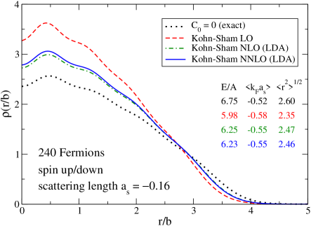
Figure 14: Density profile of a dilute system of fermions in a trap Puglia:2002vk .

Given (94) and (95), the iteration procedure is:

1. Guess an initial density profile $\rho(r)$ (e.g., the Thomas-Fermi density).

2. Evaluate the local single-particle potential ${V_{\rm KS}(r)\equiv v_{\rm ext}(r)-J_{0}(r)}$.

3. Find the wave functions and energies $\{\psi_{\alpha},\epsilon_{\alpha}\}$ of the lowest $A$ states (including degeneracies) by solving:

   $$\bigl{[}-\frac{{\nabla}^{2}}{2M}+V_{\rm KS}(r)\bigr{]}\,\psi_{\alpha}({\bf x})=\epsilon_{\alpha}\psi_{\alpha}({\bf x})\;.$$ (96)

4. Compute a new density $\rho(r)=\sum_{\alpha=1}^{A}|\psi_{\alpha}({\bf x})|^{2}$. Other observables are simple functionals of $\{\psi_{\alpha},\epsilon_{\alpha}\}$.

5. Repeat 2.–4. until changes are small (“self-consistent”)

This sounds like a simple Hartree calculation! Results at different EFT orders for a dilute Fermi gas in a harmonic oscillator trap is given in Fig. 14. Note the systematic progression from order to order.

An important consequence of the systematic EFT approach is that we can also estimate individual terms in energy functionals. If we scale contributions to the energy per particle according to the average density or $\langle k_{\rm F}\rangle$, we can make estimates Puglia:2002vk ; Bhattacharyya:2004qm . This is shown in Fig. 15 for both the dilute trapped fermions, which is under complete control, and for phenomenological energy functionals for nuclei, to which a postulated QCD power counting is applied. In both cases, the estimates agree well with the actual numbers (sometimes overestimating the contribution because of accidental cancellations), which means that truncation errors are understood.

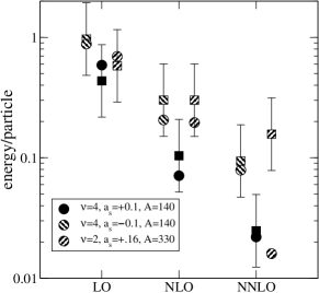
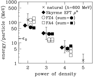
Figure 15: Estimates for energy functionals for a dilute fermions in a harmonic trap (left) and for phenomenological energy functionals for nuclei (right).

Conventional DFT is one example of using effective actions, which feature sources coupled to composite operators. It’s possible that for some applications a different type of effective action may be better. There are many outstanding questions from the present discussion, particularly as we try to adapt it to real nuclei. We’ll address some of them in the next lecture.

3 Refinements: Toward EFT/DFT for Nuclei

Let’s enumerate some questions about DFT and nuclear structure.

• How is Kohn-Sham DFT more than mean field? That is, where are the approximations and how do we truncate? How do we include long-range effects (correlations)?

• What can you calculate in a DFT approach? Can we calculate single-particle properties? Or excited states?

• How does pairing work in DFT? Can we (should we) decouple $pp$ and $ph$? Are higher-order contributions important?

• The Skyrme functional depends on multiple densities: $\rho({\bf x})$, $\tau({\bf x})$, and ${\bf J}({\bf x})$; how does that work?

• What about broken symmetries that arise with self-bound systems? (translation, rotation, …)

• How do we connect to the free, microscopic NN$\cdots$N interactions? Can we use chiral EFT or low-momentum interactions/RG?

We’ll explore some answers to these questions (and note which ones are open) in this lecture.

Consider Kohn-Sham DFT compared to the Thomas-Fermi energy functional, for which the entire functional is treated in the local density approximation (LDA). In Kohn-Sham DFT, treating kinetic energy non-locally leads to the shell structure of electrons in atoms and in trapped atoms, as seen in Fig. 16. This motivates going even further beyond the LDA.

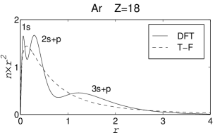
Figure 16: Thomas-Fermi vs. DFT for atoms ARGAMAN00 (left) and trapped fermions (right).

As a simple step beyond Kohn-Sham LDA, we consider functionals of the kinetic energy density in addition to the usual fermion density. The phenomenological Skyrme $E$ is a functional of $\rho$ and $\tau\equiv\langle\bm{\nabla}\psi^{\dagger}\cdot\bm{\nabla}\psi\rangle$ (and ${\bf J}$):

$$E[\rho,\tau,{\bf J}] \!=\! \int\!d^{3}x\,\biggl{\{}{1\over 2M}\tau+{3\over 8}t_{0}\rho^{2}+{1\over 16}t_{3}\rho^{2+\alpha}+{1\over 16}(3t_{1}+5t_{2})\rho\tau$$ (97)

$$\hbox{}+{1\over 64}(9t_{1}-5t_{2})(\bm{\nabla}\rho)^{2}-{3\over 4}W_{0}\rho\bm{\nabla}\cdot{\bf J}+{1\over 32}(t_{1}-t_{2}){\bf J}^{2}\biggr{\}}\;.$$

To do this in DFT/EFT, add to the Lagrangian $\eta({\bf x})\,\bm{\nabla}\psi^{\dagger}\bm{\nabla}\psi$ and generalize our Legendre transformation and inversion to $\Gamma[\rho,\tau]$,

$$\Gamma[\rho,\tau]=W[J,\eta]-\int\!J(x)\rho(x)-\int\!\eta(x)\tau(x)\;.$$ (98)

Now there are two Kohn-Sham potentials:

$$J_{0}({\bf x})=\frac{\delta\Gamma_{\rm int}[\rho,\tau]}{\delta\rho({\bf x})}\quad\mbox{and}\quad\eta_{0}({\bf x})=\frac{\delta\Gamma_{\rm int}[\rho,\tau]}{\delta\tau({\bf x})}\;.$$ (99)

The Kohn-Sham equation defines $1/M^{\ast}({\bf x})\equiv 1/M-2\eta_{0}({\bf x})$:

$$\Bigl{(}-\mathbf{\nabla}\cdot{\frac{1}{2M^{*}({\bf x})}}\mathbf{\nabla}+v_{\rm ext}({\bf x})-J_{0}({\bf x})\Bigr{)}\,\phi_{\alpha}({\bf x})=\epsilon_{\alpha}\,\phi_{\alpha}({\bf x})\;.$$ (100)

A simple first application is to evaluate Hartree-Fock diagrams including the quadratic gradient terms Bhattacharyya:2004qm . Consider the HF “bowtie diagrams”

that have vertices with derivatives:

$${\cal L}_{\rm eft}=\ldots+\frac{{C_{2}}}{16}\bigl{[}(\psi\psi)^{\dagger}(\psi\!\stackrel{{\scriptstyle\leftrightarrow}}{{\nabla}}\!{}^{2}\psi)+\mbox{ h.c.}\bigr{]}+\frac{{C_{2}^{\prime}}}{8}(\psi\!\stackrel{{\scriptstyle\leftrightarrow}}{{\nabla}}\!\psi)^{\dagger}\cdot(\psi\!\stackrel{{\scriptstyle\leftrightarrow}}{{\nabla}}\!\psi)+\ldots$$ (101)

The energy density in Kohn-Sham LDA is

$${\cal E}_{\rm int}[\rho]=\ldots+\frac{C_{2}}{8}\Bigl{[}\frac{3}{5}\left(\frac{6\pi^{2}}{\nu}\right)^{2/3}\rho^{8/3}\Bigr{]}+\frac{3C_{2}^{\prime}}{8}\Bigl{[}\frac{3}{5}\left(\frac{6\pi^{2}}{\nu}\right)^{2/3}\rho^{8/3}\Bigr{]}+\ldots$$ (102)

while the energy density in Kohn-Sham with $\tau$ ($\nu=2$) is

$${\cal E}_{\rm int}[\rho,\tau]=\ldots+\frac{C_{2}}{8}\bigl{[}\rho\tau+\frac{3}{4}(\bm{\nabla}\rho)^{2}\bigr{]}+\frac{3C_{2}^{\prime}}{8}\bigl{[}\rho\tau-\frac{1}{4}(\bm{\nabla}\rho)^{2}\bigr{]}+\ldots$$ (103)

We find that power counting estimates for terms in the energy functional also work with gradient terms (see Fig. 17).

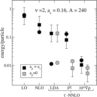
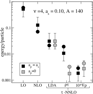
Figure 17: Estimates of terms in the energy functional, including those with gradients, compared to actual values Bhattacharyya:2004qm .

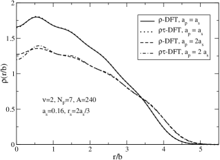
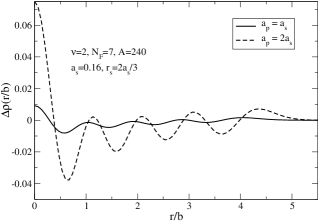
Figure 18: Comparing densities from energy functionals of $\rho$ only and $\rho$, $\tau$ Bhattacharyya:2004qm .

Now let’s compare the dilute fermion functional to the phenomenological Skyrme functional. The Skyrme energy density functional (for $N=Z$) is given in (97) while the corresponding dilute energy density functional for $\nu=4$ (and $V_{\rm external}=0$) is

$$E[\rho,\tau,{\bf J}] = \int\!d^{3}x\,\biggl{\{}{{\tau\over 2M}+{3\over 8}C_{0}\rho^{2}+{1\over 16}(3C_{2}+5C^{\prime}_{2})\rho\tau}{+{1\over 64}(9C_{2}-5C^{\prime}_{2})(\bm{\nabla}\rho)^{2}}$$ (104)

$$\hbox{}-{3\over 4}C_{2}^{\prime\prime}\rho\bm{\nabla}\cdot{\bf J}{\hbox{}+\frac{c_{1}}{2M}C_{0}^{2}\rho^{7/3}+\frac{c_{2}}{2M}C_{0}^{3}\rho^{8/3}+\frac{1}{16}D_{0}\rho^{3}}+\cdots\biggr{\}}\;.$$

They have the same terms after the association $t_{i}\leftrightarrow C_{i}$, except that the Skyrme functional is missing non-analytic terms, the three-body contribution, and other features. We note after matching to empirical Skyrme coefficients that the “effective” scattering length from $C_{0}$ is $a_{0}\approx-2\mbox{--}3\,\mbox{fm}$, but that $|k_{\rm F}a_{p}|,\,|k_{\rm F}r_{0}|<1$ (with $a_{p}<0$). However, we want the Skyrme functional to account for the finite-ranged pion, so it should not be equivalent to a short-distance expansion. Thus, the close correspondence suggests that the Skyrme functional is lacking and should be generalized.

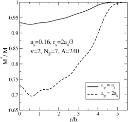
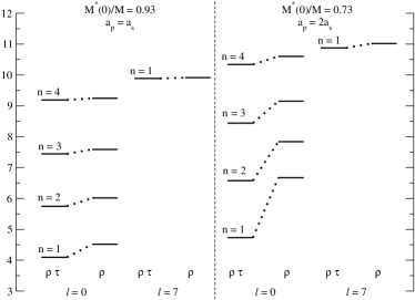
Figure 19: Comparing effective masses and single-particle spectra from energy functionals of $\rho$ only and $\rho$, $\tau$ Bhattacharyya:2004qm .

It is useful to compare results from the $\rho$ only functional compared to the $\rho$ and $\tau$ functional, as in Fig. 18 and these tables:

$a_{p}=a_{s}$	$E/A$	$\sqrt{\langle r^{2}\rangle}$
$\rho$	7.66	2.87
$\rho\tau$	7.65	2.87

$a_{p}=2a_{s}$	$E/A$	$\sqrt{\langle r^{2}\rangle}$
$\rho$	8.33	3.10
$\rho\tau$	8.30	3.09

We see very little difference in the Kohn-Sham observables, which are the binding energy and the density distribution. However, the single-particle Kohn-Sham spectrum, which is not an observable, shows significant differences, as evidenced by Fig. 19. (Note: The effective mass $M^{*}$ is closely related to single-particle levels.) We can show for a uniform system that the HF single-particle levels satisfy

$${\varepsilon_{\bf k}^{\rho}-\varepsilon_{\bf k}^{\rho\tau}}=\frac{\pi}{\nu}[(\nu-1)a_{s}^{2}r_{s}+2(\nu+1)a_{p}^{3}]\,\frac{k_{F}^{2}-{\bf k}^{2}}{2M}\rho\;,$$ (105)

and the $\rho\tau$ result is the one corresponding to the spectrum from the full Hartree-Fock propagator. So the issue becomes how the full $G$ (as shown below with the self-energy) is related to the Kohn-Sham $G_{\rm ks}$ Bhattacharyya:2004aw ; the closer they are, the better approximation $G_{\rm ks}$ will provide for single-particle properties.

$\Longrightarrow$

To explore this connection, we add a non-local source $\xi(x^{\prime},x)$ coupled to $\psi(x)\psi^{\dagger}(x^{\prime})$ [we’re back in Minkowski space here for no particular reason!]:

$$Z[J,\xi]=e^{iW[J,\xi]}=\int\!D\psi D\psi^{\dagger}\ e^{i\int\!d^{4}x\ [{\cal L}\,+\,J(x)\psi^{\dagger}(x)\psi(x)\,{+\,\int\!d^{4}x^{\prime}\,\psi(x)\xi(x,x^{\prime})\psi^{\dagger}(x^{\prime})}]}\;.$$ (106)

Writing $\Gamma[\rho,\xi]=\Gamma_{0}[\rho,\xi]+\Gamma_{\rm int}[\rho,\xi]$,

$$G(x,x^{\prime})=\left.\frac{\delta W}{\delta\xi}\right|_{J}=\left.\frac{\delta\Gamma}{\delta\xi}\right|_{\rho}=G_{\rm ks}(x,x^{\prime})+G_{\rm ks}\Bigl{[}\frac{1}{i}\frac{\delta\Gamma_{\rm int}}{\delta G_{\rm ks}}+\frac{\delta\Gamma_{\rm int}}{\delta\rho}\Bigr{]}G_{\rm ks}\;,$$ (107)

which is represented diagrammatically as:

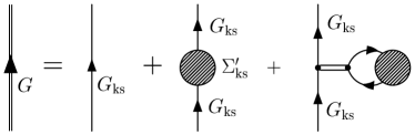
Figure 20: Full Green’s function $G$ in terms of the Kohn-Sham Green’s function $G_{\rm ks}$.

Now $G$ and $G_{\rm ks}$ yield the same density by construction; that is, $\rho_{\rm ks}({\bf x})=-i\nu G_{\rm KS}^{0}(x,x^{+})$ equals $\rho({\bf x})=-i\nu G(x,x^{+})$. Here is a simple diagrammatic demonstration (the double line is minus the inverse of a single ph ring):

But other single-particle properties (e.g., the spectrum) are generally different, since the last two terms in Fig. 20 will not cancel.

We can ask whether the Kohn-Sham basis is a useful one for $G$. Or, more simply, ask how close is $G_{\rm KS}$ to $G$. We find that it depends on what sources are used, as shown by the comparison of single-particle spectra in (105), with more sources implying less difference. This is a topic that merits further investigation.

Figure 21: Schematic momentum occupation number $n(k)$ for mean-field (Hartree-Fock) and with correlations.

The comparison of Kohn-Sham DFT and “mean-field” models often leads to misunderstandings, as when considering “occupation numbers”, because of a confusion between $G$ and $G_{\rm KS}$. Figure 21 suggests that occupation numbers are equal to 0 or 1 if and only if correlations are not included. The Kohn-Sham propagator always has a “mean-field” structure, which means that (in the absence of pairing) the Kohn-Sham occupation numbers are always 0 or 1. But correlations are certainly included in $\Gamma[\rho]$! (In principle, all correlations can be included; in practice, certain types like long-range particle-hole correlations may be largely omitted.) Further, $n({\bf k})=\langle a^{\dagger}_{\bf k}a^{\phantom{\dagger}}_{\bf k}\rangle$ is resolution dependent (not an observable!); the operator related to experiment is more complicated. Additional discussion on these issues can be found in Furnstahl:2001xq .

3.1 Pairing in Kohn-Sham DFT

There is abundant evidence for pairing in nuclei. The semi-empirical mass formula reproduces nuclear masses only with a pairing term (the last one):

$$B(N,Z) = (15.6\,\mbox{MeV})\left[1-1.5\left(\frac{N-Z}{A}\right)^{2}\right]A-(17.2\,\mbox{MeV})A^{2/3}$$ (108)

$$\hbox{}-(0.70\,\mbox{MeV})\frac{Z^{2}}{A^{1/3}}+(6\,\mbox{MeV})[(-1)^{N}+(-1)^{Z}]/A^{1/2}\;,$$

which implies an odd-even staggering of binding energies (left panel of Fig. 22). Other evidence is the energy gap in the spectra of deformed nuclei, low-lying $2^{+}$ states in even nuclei (right panel of Fig. 22), and deformations and moments of inertia (the theory requires pairing to reproduce data).

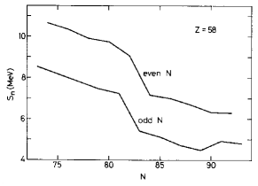
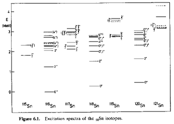
Figure 22: Evidence for pairing in nuclei (see text and RINGSCHUCK ).

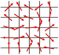
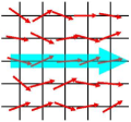
Figure 23: Spontaneous symmetry breaking analogy with spins.

Pairing is an example of spontaneous symmetry breaking, which is naturally accommodated in an effective action framework. For example, consider testing for zero-field magnetization $M$ in a spin system by introducing an external field $H$ to break the rotational symmetry. Legendre transform the Helmholtz free energy $F(H)$:

$$\mbox{\normalsize invert\ \ }M=-\partial F(H)/\partial H\quad\Longrightarrow\quad\Gamma[M]=F[H(M)]+MH(M)\;.$$ (109)

Since $H=\partial\Gamma/\partial M\longrightarrow 0$, we look for the stationary points of $\Gamma$ to identify possible ground states, including whether the symmetry broken state is lowest.

For pairing, the broken symmetry is a $U(1)$ [phase] symmetry. The textbook effective action treatment in condensed matter is to introduce a contact interaction NAGAOSA ; STONE : $g\,\psi^{\dagger}\psi^{\dagger}\psi\psi$, and perform a Hubbard-Stratonovich transformation with an auxiliary pairing field $\hat{\Delta}(x)$ coupled to $\psi^{\dagger}\psi^{\dagger}$, which eliminates the contact interaction. Then one constructs the 1PI effective action $\Gamma[\Delta]$ with $\Delta=\langle\hat{\Delta}\rangle$, and looks for values for which $\delta\Gamma/\delta\Delta=0$. To leading order in the loop expansion (mean field), this yields the BCS weak-coupling gap equation with gap $\Delta$.

The natural alternative here is to combine an expansion (e.g., EFT power counting) and the inversion method for effective actions Fukuda:im ; VALIEV97 ; VALIEV . Thus we introduce another external current $j(x)$, which is coupled to the fermion pair density in order to explicitly breaks the phase symmetry. This is a natural generalization of Kohn-Sham DFT Bulgac:2001ai ; Bulgac:2001ei ; Yu:2002kc . cf. DFT with nonlocal source OLIVEIRA88 ; KURTH99 .

So we consider a local composite effective action with pairing Furnstahl:2006pa . The generating functional has sources $J,j$ coupled to the corresponding densities:

$$Z[J,\/j]=e^{-W[J,\/j]}=\int\!D(\psi^{\dagger}\psi)\,e^{-\!\int\!d^{4}x\ [{\cal L}+J(x)\,\psi_{\alpha}^{\dagger}\psi_{\alpha}+{j(x)(\psi^{\dagger}_{\uparrow}\psi^{\dagger}_{\downarrow}+\psi_{\downarrow}\psi_{\uparrow})}]}\;.$$ (110)

Densities are found by functional derivatives with respect to $J$ and $j$:

$$\rho(x)\equiv\langle\psi^{\dagger}(x)\psi(x)\rangle_{J,j}=\left.\frac{\delta W[J,j]}{\delta J(x)}\right|_{j}\;,$$ (111)

and

$${\phi(x)\equiv\langle\psi^{\dagger}_{\uparrow}(x)\psi^{\dagger}_{\downarrow}(x)+\psi_{\downarrow}(x)\psi_{\uparrow}(x)\rangle_{J,j}=\left.\frac{\delta W[J,j]}{\delta j(x)}\right|_{J}}\;.$$ (112)

The effective action $\Gamma[\rho,\phi]$ follows as before by functional Legendre transformation:

$$\Gamma[\rho,\phi]=W[J,j]-\int\!d^{4}x\,J(x)\rho(x)-\int\!d^{4}x\,j(x)\phi(x)\;,$$ (113)

and is proportional to the (free) energy functional $E[\rho,\phi]$; at finite temperature, the proportionality constant is $\beta$. The sources are given by functional derivatives wrt $\rho$ and $\phi$:

$$\frac{\delta E[\rho,\phi]}{\delta\rho({\bf x})}=J({\bf x})\qquad\mbox{and}\qquad\frac{\delta E[\rho,\phi]}{\delta\phi({\bf x})}=j({\bf x})\;.$$ (114)

But the sources are zero in the ground state, so we determine the ground-state $\rho({\bf x})$ and $\phi({\bf x})$ by stationarity:

$$\left.\frac{\delta E[\rho,\phi]}{\delta\rho({\bf x})}\right|_{{\rho=\rho_{\rm gs},\phi=\phi_{\rm gs}}}=\left.\frac{\delta E[\rho,\phi]}{\delta\phi({\bf x})}\right|_{{\rho=\rho_{\rm gs},\phi=\phi_{\rm gs}}}=0\;.$$ (115)

This is Hohenberg-Kohn DFT extended to pairing!

We need a method to carry out the Legendre transforms to get Kohn-Sham DFT; an obvious choice is to apply the Kohn-Sham inversion method again, with order-by-order matching in the counting parameter $\lambda$. Once again,

diagrams $$\Longrightarrow {W}[J,j,\lambda]={{W}_{0}[J,j]}+\lambda{W}_{1}[J,j]+\lambda^{2}{W}_{2}[J,j]+\cdots$$

assume $$\Longrightarrow J[\rho,\phi,\lambda]={J_{0}[\rho,\phi]}+\lambda J_{1}[\rho,\phi]+\lambda^{2}J_{2}[\rho,\phi]+\cdots$$

assume $$\Longrightarrow j[\rho,\phi,\lambda]={j_{0}[\rho,\phi]}+\lambda j_{1}[\rho,\phi]+\lambda^{2}j_{2}[\rho,\phi]+\cdots$$

derive $$\Longrightarrow {\Gamma}[\rho,\phi,\lambda]={{\Gamma}_{0}[\rho,\phi]}+\lambda{\Gamma}_{1}[\rho,\phi]+\lambda^{2}{\Gamma}_{2}[\rho,\phi]+\cdots$$

Start with the exact expressions for $\Gamma$ and $\rho$

$$\Gamma[\rho,\phi]=W[J,j]-\int\!J\,\rho-\int\!j\,\phi\;,$$ (116)

and

$$\rho(x)=\frac{\delta W[J,j]}{\delta J(x)}\,,\quad\phi(x)=\frac{\delta W[J,j]}{\delta j(x)}\;,$$ (117)

and plug in the expansions, with $\rho,\phi$ treated as order unity. Zeroth order is the Kohn-Sham system with potentials $J_{0}({\bf x})$ and $j_{0}({\bf x})$,

$$\Gamma_{0}[\rho,\phi]=W_{0}[J_{0},j_{0}]-\int\!J_{0}\,\rho-\int\!j_{0}\,\phi\;,$$ (118)

so the exact densities $\rho({\bf x})$ and $\phi({\bf x})$ are by construction

$$\rho(x)=\frac{\delta W_{0}[J_{0},j_{0}]}{\delta J_{0}(x)}\,,\quad\phi(x)=\frac{\delta W_{0}[J_{0},j_{0}]}{\delta j_{0}(x)}\;.$$ (119)

Now introduce single-particle orbitals and solve

$$\left(\begin{array}[]{cc}h_{0}({\bf x})-\mu_{0}&j_{0}({\bf x})\\ j_{0}({\bf x})&-h_{0}({\bf x})+\mu_{0}\end{array}\right)\left(\begin{array}[]{c}u_{i}({\bf x})\\ v_{i}({\bf x})\end{array}\right)=E_{i}\left(\begin{array}[]{c}u_{i}({\bf x})\\ v_{i}({\bf x})\end{array}\right)$$ (120)

where

$$h_{0}({\bf x})\equiv-\frac{\bm{\nabla}^{2}}{2M}+V_{\rm trap}({\bf x})-J_{0}({\bf x})\;.$$ (121)

This is just like Skyrme Hartree-Fock Bogliubov approach RINGSCHUCK .

The diagrammatic expansion of the $W_{i}$’s is the same as without pairing, except now lines in diagrams are KS Nambu-Gor’kov Green’s functions,

$${\bf G}=\left(\begin{array}[]{cc}\langle T_{\tau}\psi_{\uparrow}(x)\psi^{\dagger}_{\uparrow}(x^{\prime})\rangle_{0}&\langle T_{\tau}\psi_{\uparrow}(x)\psi_{\downarrow}(x^{\prime})\rangle_{0}\\ \langle T_{\tau}\psi^{\dagger}_{\downarrow}(x)\psi^{\dagger}_{\uparrow}(x^{\prime})\rangle_{0}&\langle T_{\tau}\psi^{\dagger}_{\downarrow}(x)\psi_{\downarrow}(x^{\prime})\rangle_{0}\end{array}\right)\equiv\left(\begin{array}[]{cc}G_{{\rm ks}}^{0}&F_{{\rm ks}}^{0}\\ {F_{{\rm ks}}^{0}}^{\dagger}&-\widetilde{G}_{{\rm ks}}^{0}\end{array}\right)\;.$$ (122)

The extra diagram shown follows from the inversion (here it removes anomalous diagrams). In frequency space, the Kohn-Sham Green’s functions are

$$G_{{\rm ks}}^{0}({\bf x},{\bf x}^{\prime};\omega)=\sum_{j}\,\left[\frac{u_{j}({\bf x})\,u_{j}^{*}({\bf x}^{\prime})}{i\omega-E_{j}}+\frac{v_{j}({\bf x}^{\prime})\,v_{j}^{*}({\bf x})}{i\omega+E_{j}}\right]\;,$$ (123)

$$F_{{\rm ks}}^{0}({\bf x},{\bf x}^{\prime};\omega)=-\sum_{j}\,\left[\frac{u_{j}({\bf x})\,v_{j}^{*}({\bf x}^{\prime})}{i\omega-E_{j}}-\frac{u_{j}({\bf x}^{\prime})\,v_{j}^{*}({\bf x})}{i\omega+E_{j}}\right]\;.$$ (124)

The Kohn-Sham self-consistency procedure involves the same iterations as in phenomenological Skyrme HF (or relativistic mean-field) when pairing is included. In terms of the orbitals, the fermion density is

$$\rho({\bf x})=2\sum_{i}\,|v_{i}({\bf x})|^{2}\;,$$ (125)

and the pair density is (warning: this is unrenormalized!)

$$\phi({\bf x})=\sum_{i}\,[u_{i}^{*}({\bf x})v_{i}({\bf x})+u_{i}({\bf x})v_{i}^{*}({\bf x})]\;.$$ (126)

The chemical potential $\mu_{0}$ is fixed by $\int\!\rho({\bf x})=A$. Diagrams for $\Gamma[\rho,\phi]\propto E_{0}[\rho,\phi]+E_{\rm int}[\rho,\phi]$ yield the Kohn-sham potentials

$$J_{0}({\bf x})\Bigr{|}_{\rho=\rho_{\rm gs}}=\left.\frac{\delta E_{\rm int}[\rho,\phi]}{\delta\rho({\bf x})}\right|_{\rho=\rho_{\rm gs}}\ \mbox{and}\quad j_{0}({\bf x})\Bigr{|}_{\phi=\phi_{\rm gs}}=\left.\frac{\delta E_{\rm int}[\rho,\phi]}{\delta\phi({\bf x})}\right|_{\phi=\phi_{\rm gs}}\;.$$ (127)

3.2 Renormalization of Pairing

When we carry out the DFT pairing calculation for a uniform dilute Fermi system, we find divergences almost immediately. The generating functional with constant sources ${\mu}$ and ${j}$ is:

$$e^{-W[\mu,j]} = \int\!D(\psi^{\dagger}\psi)\exp\Bigl{\{}-\!\int\!d^{4}x\ \bigl{[}\psi_{\alpha}^{\dagger}(\frac{\partial}{\partial\tau}-\frac{\bm{\nabla}^{\,2}}{2M}-{\mu})\psi_{\alpha}\,$$ (129)

$$\hskip 14.45377pt\hbox{}+\frac{C_{0}}{2}\psi^{\dagger}_{\uparrow}\psi^{\dagger}_{\downarrow}\psi_{\downarrow}\psi_{\uparrow}+\,{j}(\psi_{\uparrow}\psi_{\downarrow}+\psi^{\dagger}_{\downarrow}\psi^{\dagger}_{\uparrow}){\bigr{]}\Bigr{\}}}{+\frac{1}{2}\zeta\,j^{2}}\,\bigr{]}\Bigr{\}}$$

(cf. adding an integration over an auxiliary field $\int\!D(\Delta^{\ast},\Delta)\ e^{-\frac{1}{|C_{0}|}\int\!|\Delta|^{2}}$, then shifting variables to eliminate $\psi^{\dagger}_{\uparrow}\psi^{\dagger}_{\downarrow}\psi_{\downarrow}\psi_{\uparrow}$ for $\Delta^{\ast}\psi_{\uparrow}\psi_{\downarrow}$). There are new divergences because of $j$, e.g., expand $W$ to ${\cal O}(j^{2})$:

which has the same linear divergence as in 2-to-2 scattering. To renormalize, we add the counterterm $\frac{1}{2}\zeta|j|^{2}$ to ${\cal L}$ (see ZINNJUSTIN ), which is additive to $W$ (cf. $|\Delta|^{2}$), so there is no effect on scattering.

We’ll use dimensional regularization again, but generalize from DR/MS (as used by Papenbrock and Bertsch PaB99 ) to DR/PDS, which generates explicit $\Lambda$ dependence to “check” renormalization (by verifying that $\Lambda$ dependence cancels). The basic free-space integral in $D$ spatial dimensions is

$$\left(\frac{\Lambda}{2}\right)^{3-D}\int\!\frac{d^{D}k}{(2\pi)^{D}}\,\frac{1}{p^{2}-k^{2}+i\epsilon}\stackrel{{\scriptstyle{\rm PDS}}}{{\longrightarrow}}-\frac{1}{4\pi}(\Lambda+ip)\;,$$ (130)

where $\int\!\frac{1}{\epsilon_{k}^{0}}\rightarrow\frac{M\Lambda}{2\pi}$. Renormalizing and matching free-space scattering yields for $C_{0}(\Lambda)$:

$$C_{0}(\Lambda)=\frac{4\pi a_{s}}{M}\frac{1}{1-a_{s}\Lambda}={\frac{4\pi a_{s}}{M}}+{\frac{4\pi a_{s}^{2}}{M}\Lambda}+{\cal O}(\Lambda^{2})={C_{0}^{(1)}}+{C_{0}^{(2)}}+\cdots$$ (131)

Note: we recover DR/MS by taking $\Lambda=0$. As an exercise, you can verify that NLO renormalization in free space (left):

$\Longrightarrow$  

implies that the corresponding sum of diagrams at finite density (right) is independent of $\Lambda$.

Now consider the Kohn-Sham noninteracting system for a uniform system, where we have constant chemical potential $\mu_{0}$ and pairing source $j_{0}$ (rather than spatially dependent sources). The bare density $\rho$ is:

$$\rho=-\frac{1}{\beta V}\frac{\partial W_{0}[\mu_{0},j_{0}]}{\partial\mu_{0}}=\frac{2}{V}\sum_{\bf k}v_{k}^{2}=\int\!\frac{d^{3}k}{(2\pi)^{3}}\,\biggl{(}1-\frac{\epsilon_{k}^{0}-\mu_{0}}{E_{k}}\biggr{)}\;,$$ (132)

and the bare pair density $\phi_{B}$ is:

$$\phi_{B}=\frac{1}{\beta V}\frac{\partial W_{0}[\mu_{0},j_{0}]}{\partial j_{0}}=\frac{2}{V}\sum_{\bf k}u_{k}v_{k}=-\int\!\frac{d^{3}k}{(2\pi)^{3}}\,\frac{j_{0}}{E_{k}}\;.$$ (133)

In these expressions, $j_{0}$ plays role of constant gap; e.g., the spectrum is

$${E_{k}=\sqrt{(\epsilon_{k}^{0}-\mu_{0})^{2}+j_{0}^{2}}}\;,\qquad\epsilon_{k}^{0}=\frac{k^{2}}{2M}\;.$$ (134)

(See also Fig. 24.) The divergence in $\phi_{B}$ is illustrated in Fig. 25.

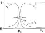
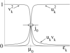
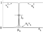
Figure 24: Quasiparticle wave functions for a uniform system for several values of $j_{0}/\mu_{0}$. As $j_{0}/\mu_{0}$ decreases, $u_{k}v_{k}$ becomes sharply peaked at $\mu_{0}$.

Figure 25: Illustration of the divergence in $\sum_{k}u_{k}v_{k}$.

The basic DR/PDS integral in $D$ dimensions, with $x\equiv j_{0}/\mu_{0}$, is

$${I(\beta)} \equiv \Bigl{(}\frac{\Lambda}{2}\Bigr{)}^{3-D}\int\!\frac{d^{D}k}{(2\pi)^{D}}\,\frac{(\epsilon_{k}^{0})^{\beta}}{\sqrt{(\epsilon_{k}^{0}-\mu_{0})^{2}+j_{0}^{2}}}$$ (135)

$$= {\frac{M\Lambda}{2\pi}\,\mu_{0}^{\beta}\,\Bigl{(}1-\delta_{\beta,2}\frac{x^{2}}{2}\Bigr{)}}$$

$$\quad\hbox{}+(-)^{\beta+1}\,\frac{M^{3/2}}{\sqrt{2}\pi}\,[\mu_{0}^{2}(1+x^{2})]^{(\beta+1/2)/2}\,P^{0}_{\beta+1/2}\Bigl{(}\frac{-1}{\sqrt{1+x^{2}}}\Bigr{)}\;.$$

We can check that in the KS density equation the $\Lambda$ dependence cancels:

$${\rho}=-\frac{1}{\beta V}\frac{\partial W_{0}[\,]}{\partial\mu_{0}}=\int\!\frac{d^{3}k}{(2\pi)^{3}}\,\biggl{(}1-\frac{\epsilon_{k}^{0}}{E_{k}}+\frac{\mu_{0}}{E_{k}}\biggr{)}\longrightarrow{0-I(1)+\mu_{0}\,I(0)}\;.$$ (136)

The KS equation for the pair density $\phi$ fixes $\zeta^{(0)}$:

$${\phi}=\frac{1}{\beta V}\frac{\partial W_{0}[\,]}{\partial j_{0}}=-\int\!\frac{d^{3}k}{(2\pi)^{3}}\,\frac{j_{0}}{E_{k}}+\zeta^{(0)}j_{0}\longrightarrow{-j_{0}\,I(0)+\zeta^{(0)}j_{0}}$$ (137)

so that

$$\zeta^{(0)}=\frac{M\Lambda}{2\pi}\;.$$ (138)

Calculating to $n^{\rm th}$ order, we find $\Gamma_{1\leq i\leq n}[\rho,\phi]$ by first constructing all of the $W_{1\leq i\leq n}[\mu_{0}(\rho,\phi),j_{0}(\rho,\phi)]$, including additional Feynman rules VALIEV ,

So the procedure is to calculate $\mu_{i}$, $j_{i}$ from $\Gamma_{i}$, then use $\sum_{i=0}^{n}j_{i}=j\rightarrow 0$ to find $j_{0}$. The renormalization conditions mean that there is no freedom in choosing $C_{0}(\Lambda)$, so the $\Lambda$’s must cancel! In leading order, diagrams for $\Gamma_{1}[\rho,\phi]=W_{1}[\mu_{0}(\rho,\phi),j_{0}(\rho,\phi)]$ are

and we choose $\delta Z_{j}^{(n)}$ and $\zeta^{(n)}$ to convert $\phi_{B}$ to the renormalized $\phi$, yielding

$${\frac{1}{\beta V}\Gamma_{1}[\rho,\phi]=\frac{1}{4}C_{0}^{(1)}\rho^{2}+\frac{1}{4}C_{0}^{(1)}\phi^{2}}\quad\mbox{with\ }C_{0}^{(1)}=\frac{4\pi a_{s}}{M}\;.$$ (139)

The $\Gamma_{1}$ dependence on $\rho$ and $\phi$ is explicit, so it is easy to find $\mu_{1}$ and $j_{1}$:

$$\mu_{1}=\frac{1}{\beta V}\frac{\partial\Gamma_{1}}{\partial\rho}=\frac{1}{2}C_{0}^{(1)}\rho\qquad\mbox{and}\qquad j_{1}=-\frac{1}{\beta V}\frac{\partial\Gamma_{1}}{\partial\phi}=-\frac{1}{2}C_{0}^{(1)}\phi\;.$$ (140)

The “gap” equation then follows from $j=j_{0}+j_{1}=0$:

$$j_{0}=-j_{1}=-\frac{1}{2}|C_{0}^{(1)}|\phi=\frac{1}{2}|C_{0}^{(1)}|\,j_{0}\left[\int\!\frac{d^{3}k}{(2\pi)^{3}}\,\frac{1}{\sqrt{(\epsilon_{k}^{0}-\mu_{0})^{2}+j_{0}^{2}}}-\zeta^{(0)}\right]\;.$$ (141)

DR/PDS reproduces the Papenbrock/Bertsch result PaB99 (with $x\equiv|j_{0}/\mu_{0}|$)

$$1 = -\sqrt{2M\mu_{0}}|a_{s}|(1+x^{2})^{1/4}P^{0}_{1/2}\left(\frac{-1}{\sqrt{1+x^{2}}}\right)$$ (142)

$$\stackrel{{\scriptstyle x\rightarrow 0}}{{\longrightarrow}}k_{\rm F}a_{s}\Bigl{[}\frac{4-6\log{2}}{\pi}+\frac{2}{\pi}\log{x}\Bigr{]}\;,$$

and if $k_{\rm F}a_{s}<1$, then $j_{0}/\mu_{0}=(8/e^{2})e^{-\pi/2k_{\rm F}|a_{s}|}$ holds to very good approximation.

The renormalized effective action $\Gamma=\Gamma_{0}+\Gamma_{1}$ is

$$\frac{1}{\beta V}\Gamma=\int\!(\epsilon_{k}^{0}-\mu_{0}-E_{k})+\frac{1}{2}\zeta^{(0)}j_{0}^{2}+\mu_{0}\rho-j_{0}\phi+\frac{1}{4}C_{0}^{(1)}\rho^{2}+\frac{1}{4}C_{0}^{(1)}\phi^{2}\;.$$ (143)

We check for $\Lambda$’s again,

$$\frac{1}{\beta V}\Gamma=0-I(2)+2\mu_{0}I(1)-(\mu_{0}^{2}+j_{0}^{2})I(0)+\frac{1}{2}\frac{M\Lambda}{2\pi}j_{0}^{2}+\cdots$$ (144)

and find they do cancel:

$$\frac{M\Lambda}{2\pi}\Bigl{(}-\mu_{0}^{2}(1-j_{0}^{2}/2\mu_{0}^{2})+2\mu_{0}^{2}-\mu_{0}^{2}-j_{0}^{2}+\frac{1}{2}j_{0}^{2}\Bigr{)}=0\;.$$ (145)

To find the energy density, evaluate $\Gamma$ at the stationary point $j_{0}=-\frac{1}{2}|C_{0}^{(1)}|\phi$ with $\mu_{0}$ fixed by the equation for $\rho$, yielding the same results as Papenbrock/Bertsch (plus an HF term) Furnstahl:2006pa .

Figure 26: Contributions to the NLO energy density.

Life gets more complicated at Next-to-Leading Order (NLO), where dependence of $\Gamma_{2}$ on $\rho$ and $\phi$ is no longer explicit and analytic formulas for DR integrals not available. $\Gamma_{2}$ at NLO is Furnstahl:2006pa

$$-\bigl{(}C_{0}^{(1)}\bigr{)}^{2}\int\!\!\frac{d^{3}p}{(2\pi)^{3}}\int\!\!\frac{d^{3}k}{(2\pi)^{3}}\int\!\!\frac{d^{3}q}{(2\pi)^{3}}\frac{1}{E_{p}+E_{k}+E_{p-q}+E_{k+q}}$$

$$\qquad\qquad\hbox{}\times\bigl{[}\,{u_{p}^{2}\,u_{k}^{2}\,v_{p-q}^{2}\,v_{k+q}^{2}}-2u_{p}^{2}\,v_{k}^{2}\,(uv)_{p-q}\,(uv)_{k+q}$$

$$\qquad\qquad\qquad\hbox{}+(uv)_{p}\,(uv)_{k}\,(uv)_{p-q}\,(uv)_{k+q}\,\bigr{]}$$ (146)

and

$$-\bigl{(}C_{0}^{(1)}\bigr{)}^{2}\int\!\!\frac{d^{3}k}{(2\pi)^{3}}\,\frac{1}{2E_{k}}\bigl{[}\rho(u_{k}v_{k})^{2}+\frac{1}{2}{\phi_{B}}({u_{k}^{2}}-v_{k}^{2})\bigr{]}^{2}\;.$$ (147)

The UV divergences can be identified from

$$v_{k}^{2}=\frac{1}{2}\left(1-\frac{\xi_{k}}{E_{k}}\right)\stackrel{{\scriptstyle k\rightarrow\infty}}{{\longrightarrow}}\frac{j_{0}^{2}M^{2}}{k^{4}}\;,\qquad u_{k}^{2}=\frac{1}{2}\left(1+\frac{\xi_{k}}{E_{k}}\right)\stackrel{{\scriptstyle k\rightarrow\infty}}{{\longrightarrow}}1-\frac{j_{0}^{2}M^{2}}{k^{4}}\;,$$ (148)

and

$$u_{k}v_{k}=-\frac{j_{0}}{2E_{k}}\stackrel{{\scriptstyle k\rightarrow\infty}}{{\longrightarrow}}-\frac{j_{0}M}{k^{2}}\;,\qquad\qquad\frac{1}{E_{k}}\stackrel{{\scriptstyle k\rightarrow\infty}}{{\longrightarrow}}\frac{2M}{k^{2}}\;.$$ (149)

For the renormalization at NLO to work, the bowtie diagram with the $C_{0}^{(2)}=(4\pi a_{s}^{2}/M)\Lambda$ vertex must precisely cancel the $\Lambda$ dependence from the beachball with $C_{0}^{(1)}=4\pi a_{s}/M$ vertices:

(Note that the $\delta Z_{j}^{(1)}$ vertex takes $\phi_{B}\rightarrow\phi$.) How do we see cancellation of $\Lambda$’s and evaluate renormalized results without analytic formulas?

Before addressing that issue, we first see how the standard induced interaction result GORKOV61 ; HEISELBERG00 is recovered here. As $j_{0}\rightarrow 0$, $u_{k}v_{k}$ peaks at $\mu_{0}$ (see Fig. 24). At leading order (for $T=0$),

$$\Delta_{LO}/\mu_{0}=\frac{\ts 8}{\ts e^{2}}\,e^{-1/N(0)|C_{0}|}=\frac{\ts 8}{\ts e^{2}}\,e^{-\pi/2k_{\rm F}|a_{s}|}\;,$$ (150)

where we make the association $j_{0}\rightarrow\Delta_{LO}$. At NLO the exponent is modified, which changes the prefactor, $\Delta_{NLO}\approx\Delta_{LO}/(4e)^{1/3}$, using

Further details can be found in Furnstahl:2006pa . An unexplored question is how does the Kohn-Sham gap compare to “real” gap?

Now we return to the question of renormalizing in practice; an alternative approach is to use subtractions. The NLO integrals with $E_{k}=\sqrt{(\epsilon_{k}-\mu_{0})^{2}+j_{0}^{2}}$ are intractable, but we directly obtain a renormalized result with the substitution

$$\int\!\frac{1}{E_{1}+E_{2}+E_{3}+E_{4}}\longrightarrow\int\biggl{[}{\frac{1}{E_{1}+E_{2}+E_{3}+E_{4}}-\frac{{\cal P}}{\epsilon^{0}_{1}+\epsilon^{0}_{2}-\epsilon^{0}_{3}-\epsilon^{0}_{4}}}\biggr{]}$$ (151)

plus a DR/PDS integral that is proportional to $\Lambda$. When applied at LO,

$$\int\!\frac{1}{E_{k}}=\int\!\Bigl{[}{\frac{1}{E_{k}}-\frac{\cal P}{\epsilon^{0}_{k}}}\Bigr{]}+\frac{M\Lambda}{2\pi}\;.$$ (152)

This is the same sort of subtraction used to eliminate $C_{0}$ in the gap equation,

$$\frac{M}{4\pi a_{s}}+\frac{1}{|C_{0}|}=\frac{1}{2}\int\!\frac{d^{3}k}{(2\pi)^{3}}\,\frac{1}{\epsilon_{k}^{0}}\Longrightarrow\frac{M}{4\pi a_{s}}=-\frac{1}{2}\int\!\frac{d^{3}k}{(2\pi)^{3}}\,\biggl{[}\frac{1}{E_{k}}-\frac{1}{\epsilon_{k}^{0}}\biggr{]}\;.$$ (153)

Any equivalent subtraction also works, e.g.,

$$\int\!\frac{d^{3}k}{(2\pi)^{3}}\,\frac{\cal P}{\epsilon^{0}_{k}-\mu_{0}}=\int\!\frac{d^{3}k}{(2\pi)^{3}}\,\frac{1}{\epsilon^{0}_{k}}\;.$$ (154)

So how do we renormalize the divergent pair (anomalous) density,

$$\phi({\bf x})=\sum_{i}\,[u_{i}^{*}({\bf x})v_{i}({\bf x})+u_{i}({\bf x})v_{i}^{*}({\bf x})]\longrightarrow\infty\;,$$ (155)

in a finite system? (Cf. the scalar density $\rho_{s}=\sum_{i}\overline{\psi}({\bf x})\psi({\bf x})$ for relativistic Hartree theory). Answer: use the subtracted expression for $\phi$ in the uniform system,

$$\phi=\int^{k_{c}}\!\frac{d^{3}k}{(2\pi)^{3}}\,j_{0}\left(\frac{1}{\sqrt{(\epsilon_{k}^{0}-\mu_{0})^{2}+j_{0}^{2}}}-\frac{1}{\epsilon_{k}^{0}}\right)\stackrel{{\scriptstyle k_{c}\rightarrow\infty}}{{\longrightarrow}}\mbox{finite,}$$ (156)

and apply this in a local density approximation (Thomas-Fermi):

$$\phi({\bf x})=2\sum_{i}^{E_{c}}u_{i}({\bf x})v_{i}({\bf x})-j_{0}({\bf x})\frac{M\,{k_{c}({\bf x})}}{2\pi^{2}}\quad\mbox{with}\quad{E_{c}=\frac{k_{c}^{2}({\bf x})}{2M}+J({\bf x})-\mu_{0}}\;.$$ (157)

This procedure was worked out by Bulgac and collaborators Bulgac:2001ei ; Bulgac:2001ai ; Yu:2002kc . Convergence is very slow as the energy cutoff is increased, so Bulgac/Yu devised a different subtraction,

$$\phi=\int^{k_{c}}\!\frac{d^{3}k}{(2\pi)^{3}}\,j_{0}\left(\frac{1}{\sqrt{(\epsilon_{k}^{0}-\mu_{0})^{2}+j_{0}^{2}}}{-\frac{{\cal P}}{\epsilon_{k}^{0}-\mu_{0}}}\right)\stackrel{{\scriptstyle k_{c}\rightarrow\infty}}{{\longrightarrow}}\mbox{finite}\;.$$ (158)

A comparison of convergence in uniform system for the two subtraction schemes (156) and (158):

shows dramatic improvement for the Bulgac/Yu subtraction. Bulgac et al. have demonstrated that this works in finite systems, and there have been recent practical applications.

We finish this lecture with a brief mention of alternatives to a local Kohn-Sham formalism for pairing. One alternative is to couple a source to the non-local pair field OLIVEIRA88 ; KURTH99 :

$$\widehat{H}\longrightarrow\widehat{H}-\int\!dx\,dx^{\prime}\,[D^{*}(x,x^{\prime})\psi_{\uparrow}(x)\psi_{\downarrow}(x^{\prime})+\mbox{H.c.}]\;,$$ (159)

which yields essentially a two-particle-irreducible (2PI) effective action $\Gamma[\rho,\Delta]$ with $\Delta(x,x^{\prime})=\langle\psi_{\uparrow}(x)\psi_{\downarrow}(x^{\prime})\rangle$. Or one could use auxiliary fields: introduce $\widehat{\Delta}^{*}(x)\psi(x)\psi(x)+\mbox{H.c.}$ via a Hubbard-Stratonovich transformation to obtain a 1PI effective action in $\Delta(x)=\langle\widehat{\Delta}(x)\rangle$. By adopting a special saddle point evaluation, one can obtain Kohn-Sham DFT. Finally there is the possibility of deriving a density functional (without Kohn-Sham orbits) by direct renormalization group evolution Schwenk:2004hm .

4 Loose Ends and Challenges plus Cold Atoms

In this final lecture, we touch on some loose ends raised in previous lectures, and outline some of the plans and challenges for moving forward toward a microscopic DFT for nuclei based on effective field theory and renormalization group ideas and methods Furnstahl:2004xn . We’ll also briefly consider cold atom physics and some recent work on density functionals for that problem.

4.1 Toward a Microscopic Nuclear DFT

We have outlined a framework for generating density functional theory based on effective actions. A key ingredient is a tractable hierarchy of many-body approximations to which we can apply the inversion method. A scenario for carrying this out has emerged, which combines chiral effective field theory (EFT) interactions with renormalization group techniques. While many challenges remain, it is a plausible and systematically improvable path to a microscopic nuclear DFT.

This scenario goes like this:

1. Construct a chiral EFT to a given order, including all many-body forces. At present, the NN chiral EFT has been worked out to N³LO N3LO ; N3LOEGM , while three-body forces at the N²LO level are used. The latter will soon be extended to N³LO and already the leading four-body force (which appears at N³LO) has been tested. To minimize the truncation error following Lepage’s prescription, one should increase the cutoff regulator $\Lambda$ until the truncation error is minimized. (Note: it is still a matter of investigation where the breakdown scale actually lies.)

2. Evolve the Hamiltonian to lower $\Lambda$ with renormalization group (RG) methods. There are choices here, including the $V_{{\rm low}\,k}$ approach, the Similarity Renormalization Group (SRG) Bogner:2006pc ; Bogner:2007 , and possibly simply a direct construction of the chiral EFT at a lower cutoff Coraggio:2007mc . Cutoffs in the range of $\Lambda\approx 2\,\mbox{fm}^{-1}$ appear to be appropriate for ordinary nuclei. One needs the consistent evolution of all interactions and other operators. As discussed in the first lecture, by decoupling high and low momentum the nuclear many-body problem becomes perturbative in the particle-particle channel, in stark contrast to the situation with conventional interactions Bogner_nucmatt ; Bogner:2007 .

3. Generate the density functional in effective action form. A by-product of evolving to low momentum is that the convergence of the many-body diagrams no longer is critically dependent on the choice of single-particle potential. This opens the door to choosing it to maintain the density as in a Kohn-Sham approach. In the short term, a direct construction of the functional in the Skyrme form is possible via an adaption (and extension) of Negele and Vautherin’s density matrix expansion (DME) NEGELE72 ; NEGELE75 . In the long term, chain-rule constructions will allow non-local effects to be included [see after (88)].

This program is well underway and is part of a larger project to construct and constrain a universal nuclear energy density functional (UNEDF). A detailed overview and an explanation of the DME will be available in a forthcoming publication Platter .

We’ll briefly describe the idea of the DME NEGELE72 ; NEGELE75 , which starts by expressing the Hartree-Fock energy using the density matrix. Recall that we take the best single Slater determinant in a variational sense

$$|\Psi_{\rm HF}\rangle=\det\{\psi_{i}({\bf x}),i=1\cdots A\}\,,\quad{\bf x}=({\bf r},\sigma,\tau)\;,$$ (160)

to find the Hartree-Fock energy (suppressing $\sigma,\tau$):

$$\langle\Psi_{\rm HF}|\widehat{H}|\Psi_{\rm HF}\rangle \!\!\!\!=\!\!\!\! \cdots{+\frac{1}{2}\sum_{i,j=1}^{A}\int\!\!d{\bf r}_{1}\!\int\!\!d{\bf r}_{2}\,|\psi_{i}({\bf r}_{1})|^{2}v({\bf r}_{1},{\bf r}_{2})|\psi_{j}({\bf r}_{2})|^{2}}$$ (162)

$$\hbox{}{-\frac{1}{2}\sum_{i,j=1}^{A}\int\!\!d{\bf r}_{1}\!\int\!\!d{\bf r}_{2}\,\psi^{\dagger}_{i}({\bf r}_{1})\psi_{i}({\bf r}_{2})v({\bf r}_{1},{\bf r}_{2})\psi^{\dagger}_{j}({\bf r}_{2})\psi_{j}({\bf r}_{1})}\;.$$

We can trivially express this in terms of the single-particle density matrix:

$$\rho({\bf r}_{1},{\bf r}_{2})=\nu\sum_{\epsilon_{\alpha}\leq\epsilon_{\rm F}}\psi_{\alpha}^{\dagger}({\bf r}_{1})\psi_{\alpha}({\bf r}_{2})\;.$$ (163)

The idea is to write this in the Kohn-Sham basis (i.e., the $\psi_{\alpha}$’s are Kohn-Sham orbitals), so that it is compatible with the DFT diagrammatic expansion. If we change to ${\bf R}=\frac{1}{2}({\bf r}_{1}+{\bf r}_{2})$ and ${\bf s}={\bf r}_{1}-{\bf r}_{2}$, we can expand in ${\bf s}$

$$\rho({\bf R}+{\bf s}/2,{\bf R}-{\bf s}/2)=e^{{\bf s}\bm{\cdot}(\bm{\nabla}_{1}-\bm{\nabla}_{2})/2}\left.\rho({\bf r}_{1},{\bf r}_{2})\right|_{{\bf s}=0}\;.$$ (164)

Negele and Vautherin obtained an expansion in terms of the fermion, kinetic energy, and other densities:

$$\rho({\bf r}_{1},{\bf r}_{2})=\frac{3j_{1}(sk)}{sk}\rho({\bf R})+\frac{35j_{3}(sk)}{2sk^{3}}\left(\frac{1}{4}\nabla^{2}\rho({\bf R})-\tau({\bf R})+\frac{3}{5}k^{2}\rho({\bf R})+\cdots\right)\;,$$ (165)

which leads to functionals of these densities, for which we can take the $\delta/\delta\rho({\bf R})$, $\delta/\delta\tau({\bf R})$, etc. derivatives directly. (See also DME applied to ChPT in nuclear medium by Kaiser and collaborators Kaiser:2002jz ; Kaiser:2003uh ; Kaiser:2005 .) This is clear at the Hartree-Fock level, but generalizations are needed for higher-order diagrams. These are also in progress Vincent:2007 .

Figure 27: Long-range effects contributing to energy density functionals.

There are some important open questions for this approach or any DFT treatment of finite nuclei. These include:

• For pairing, the energy interpretation, number projection, renormalization in finite systems, and efficient numerical implementation. Also, a unified microscopic treatment of particle-particle and particle-hole physics.

• DFT for self-bound systems. Self-bound systems have no external potential, which implies that the true ground-state density is uniform! More generally, how do we deal with symmetry breaking (translational, rotational invariance, particle number) and restoration. There has been little or no guidance from Coulomb DFT. There are analogous issues and methods for effective actions, namely soliton zero modes and projection methods. Work on an energy functional for the intrinsic density is in its infancy Engel:2006qu .

• Long-range effects, as illustrated schematically in Fig. 27. This includes long-range forces (i.e., pion and Coulomb exchange) but also long-range correlations. The latter can be understood as non-localities from near-on-shell particle-hole excitations, as in the lower diagrams pictured in Fig. 27.

4.2 Covariant DFT

Thus far, our discussion has included only nonrelativistic EFT and DFT. However, there is a successful phenomenology based on relativistic mean field energy functionals SEROT86 ; RING96 ; SEROT97 . Can we make a connection?

In principle we could proceed by deriving a covariant EFT. We start by observing that all low-energy effective theories have incorrect UV behavior. Sensitivity to short-distance physics is signalled by divergences but finiteness (e.g., with cutoff) doesn’t mean there is not sensitivity! One must absorb (and correct) sensitivity by renormalization. Instances of UV divergences for low-energy nuclear physics are

nonrelativistic	covariant
scattering	scattering
pairing	pairing
	anti-nucleons

Thus, there is an additional source of divergences in the covariant case from the “Dirac sea”.

Gasser, Sainio, Svarc GASSER88 derived chiral perturbation theory (ChPT) for ${\pi}N$ physics using relativistic nucleon degrees of freedom. But they found that the loop and momentum expansions no longer agree (as they do in nonrelativistic ChPT), which means that systematic power counting was lost. The heavy-baryon EFT restores power counting by a ${1/M}$ expansion, and has been the basis for nonrelativistic NN EFT treatments JENKINS91 .

However, Hua-Bin Tang TANG96 (and with Paul Ellis ELLIS98 ) observed:

“…EFT’s permit useful low-energy expansions only if we absorb all of the hard-momentum effects into the parameters of the Lagrangian.” “When we include the nucleons relativistically, the anti-nucleon contributions are also hard-momentum effects.”

They advocated moving the “Dirac sea” physics into the coefficients, thereby absorbing the “hard” part of a diagram into parameters, while the remaining “soft” part satisfies chiral power counting. The original ${\pi}N$ prescription by Tang and Ellis (expand, integrate term-by-term, and resum propagators) was systematized for ${\pi}N$ by Becher and Leutwyler under the name “infrared regularization” or IR BECHER99 . It is not unique; e.g., Fuchs et al. have used additional finite subtractions in DR FUCHS03 . The extension of IR to multiple heavy particles by Lehmann and Prézeau Lehmann:2001xm , with a convenient reformulation by Schindler, Gegelia, and Scherer Schindler:2003xv , offers the possibility of a working covariant EFT.

If we restrict our attention to purely short-ranged, natural interactions, there are tremendous simplifications. In particular, tadpoles and $N\overline{N}$ loops in free space vanish! For example, leading order (LO) has scalar, vector, etc. vertices,

$${\cal L}_{\rm eft}=\cdots-\frac{{C_{s}}}{2}(\overline{\psi}\psi)(\overline{\psi}\psi)-\frac{{C_{v}}}{2}(\overline{\psi}\gamma^{\mu}\psi)(\overline{\psi}\gamma_{\mu}\psi)+\cdots$$ (166)

which we designate as

and consider all possible diagrams at NLO:

Only the particle-particle loop diagram survives IR and all of the others pictured here vanish. Since only forward-going nucleons contribute in the end, one obtains the same scattering amplitude as in nonrelativistic DR/MS for small $k$.

Unlike QED DFT, “no sea” for nuclear structure is a misnomer; one should include $\overline{N}N$ “vacuum physics” in coefficients via renormalization. But note that requiring renormalizability at the hadronic level corresponds to making a model for the short-distance behavior, which has proven to be a poor model phenomenologically. Fixing short-distance behavior is not the same thing as throwing away negative-energy states. For a long time, people searched for unique “relativistic effects”; these were largely misguided efforts.

The further investigation of covariant EFT and its extension to DFT is motivated by the successes of relativistic mean-field phenomenology and other arguments about low-energy QCD. But there is much to be done for it to be competitive with the nonrelativistic EFT.

4.3 DFT for Cold Atoms with Large Scattering Length

Finally we return to the large scattering length problem, which is realizable with cold atoms. The total cross section for scattering is expressed in term of partial-wave phase shifts as

$$\sigma_{\rm total}=\frac{4\pi}{k^{2}}\sum_{l=0}^{\infty}(2l+1)\sin^{2}\delta_{l}(k)\;.$$ (167)

Recall that an attractive potential pulls the asymptotic wave function (outside the potential) in, by an amount at each energy or $k$ called the phase shift. At low energy ($\lambda=2\pi/k\gg 1/R$), the S-wave phase shift $\delta_{0}(k)$ satisfies:

$$k\cot\delta_{0}(k)\stackrel{{\scriptstyle k\rightarrow 0}}{{\longrightarrow}}-\frac{1}{a_{0}}+\frac{1}{2}r_{0}k^{2}+\ldots$$ (168)

where ${a_{0}}$ is the “scattering length” and $r_{0}$ is the “effective range”. The effective range expansion for low-energy scattering goes back to Schwinger and Bethe and others. The effective range expansion typifies the general principles we have stated for EFT’s: If a complicated potential produces scattering with a given $a_{0}$ and $r_{0}$, we can replace it by a simpler potential with the same values and everything agrees at low energies. In general, the effective-range expansion is reproduced and extended by EFT.

Having a bound-state or near-bound state at zero energy means large scattering lengths ($a_{0}\rightarrow\pm\infty$). For $kR\rightarrow 0$, the total cross section is

$$\sigma_{\rm total}=\sigma_{l=0}=\frac{4\pi a_{0}^{2}}{1+(ka_{0})^{2}}=\left\{\begin{array}[]{cl}4\pi a_{0}^{2}&\mbox{for\ }ka_{0}\ll 1\;,\\ \frac{\textstyle 4\pi}{\textstyle k^{2}}&\mbox{for\ }ka_{0}\gg 1\mbox{\ (unitarity limit).}\end{array}\right.$$ (169)

We are particularly interested in cases where there is a bound-state near zero energy or there just misses being a bound state. These pictures:

are a reminder of the interpretation of the scattering length in terms of the intercept of the zero energy scattering wave function, which is a straight line outside the potential. For potentials that just have a bound state, the wave function just turns over and $a_{0}$ is large and positive. If the potential just fails to have a bound state, it doesn’t quite make it to horizontal and $a_{0}$ is large and negative.

At low energies, depending on the size of $k$ times $a_{0}$, the cross section first goes like the square of $a_{0}$ and then saturates at the unitarity limit. So if we could adjust the depth of the bound state, we can control the “strength” of the interaction in a sense. This is possible for atoms by changing an external magnetic field to produce resonant scattering. For QCD is it possible to adjust the quark mass theoretically so that $m_{\pi}$ changes and the nuclear $a_{0}$ can be tuned to $\pm\infty$!

Let’s consider the large scattering length many-body problem, which means we have an attractive two-body potential with $a_{0}\rightarrow\infty$. If $R\ll 1/k_{\rm F}\ll a_{0}$, as in this figure,

then we expect scale invariance (since we lose both $R$ and $a_{0}$ as possible scales). This means that the energy and superfluid gap should be pure numbers times $E_{\rm FG}=\frac{3}{5}\frac{k_{\rm F}^{2}}{2M}$.

Recall that for the natural scattering length case, EFT power counting led to an organized perturbative expansion:

with $C_{0}=\frac{\textstyle 4\pi}{\textstyle M}a_{0}$ and $ka_{0}\ll 1$. But in the large scattering length limit, $ka_{0}\gg 1$ so the bubble series diverges. This is not a difficulty in free space, because the geometric sum of bubbles is easily performed. This sum yields the $f_{0}(k)$ expansion by keeping $ka_{0}$ to all orders and expanding the rest:

$$f_{0}(k)\propto\frac{1}{-1/a_{0}+r_{0}k^{2}/2-ik}\longrightarrow\frac{-1}{1/a_{0}+ik}\left[1+\frac{r_{0}/2}{1/a_{0}+ik}k^{2}+\cdots\right]$$ (170)

With a natural $a_{0}$ and a perturbative expansion, we found the DR/MS (minimal subtraction) scheme particularly convenient. With large $a_{0}$, we need a new renormalization scheme. DR/PDS was proposed by Kaplan, Savage, Wise KSW and counts $\mu\sim k$:

$$\raisebox{-14.45377pt}{\includegraphics*[width=28.90755pt,angle={0}]{fig_C0}}\ \Longrightarrow\ C_{0}{(\mu)=\frac{4\pi}{M}\left(\frac{1}{-\mu+1/a_{0}}\right)\stackrel{{\scriptstyle a_{0}\rightarrow\infty}}{{\longrightarrow}}-\frac{4\pi}{M\mu}}\;,$$ (171)

$$\raisebox{-14.45377pt}{\includegraphics*[width=50.58878pt,angle={0}]{fig_C0sq}}\ \Longrightarrow\ \int\!\frac{d^{D}q}{(2\pi)^{3}}\frac{1}{k^{2}-q^{2}+i\epsilon}\stackrel{{\scriptstyle D\rightarrow 3}}{{\longrightarrow}}-\frac{{\mu+}ik}{4\pi}\;.$$ (172)

In medium, each additional $C_{0}$ vertex gives a factor

$$C_{0}(k_{\rm F})\left(\frac{M}{k_{\rm F}^{2}}\right)^{2}\left(\frac{k_{\rm F}^{5}}{M}\right)\sim k_{\rm F}^{0}\;,$$ (173)

which means that all $C_{0}$ diagrams are leading order! Thus, we are told to sum all many-body diagrams with $C_{0}$ vertices. This is only possible numerically (or possibly with an additional expansion).

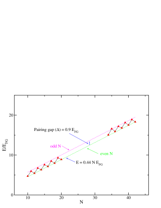
Figure 28: GFMC results from Chang et al. Chang:2004sj for the unitary fermion system.

So we turn to numerical calculations. GFMC results from Chang et al. Chang:2004sj , in which one extrapolates to large numbers of fermions, are shown in Fig. 28. They find the energy per particle is $E/N=0.44(1)E_{\rm FG}$. Diffusion Monte Carlo (DMC) results Astrak , with a square-well potential tuned to $a_{0}\rightarrow\infty$ and an extrapolation to large numbers of fermions, find a similar result, namely an energy per particle of $E/N=0.42(1)E_{\rm FG}$.

Thomas Papenbrock has considered DFT for the unitary regime Papenbrock:2005bd . He assumes a simple, constrained form of the density functional,

$${\cal E}[\rho]=\frac{\hbar^{2}}{m}\left[\frac{m}{2m_{\rm eff}}\sum_{j=1}^{N}|\nabla\phi_{j}(r)|^{2}+\Bigl{(}\xi-\frac{m}{m_{\rm eff}}\Bigr{)}c\rho^{5/3}\right]+\frac{1}{2}m\omega^{2}r^{2}\rho\;,$$ (174)

with non-localities and gradient terms via the effective mass $m_{\rm eff}$. The parameters in $E[\rho]=\int\!d{\bf x}\,{\cal E}[\rho({\bf x})]$ can be fit for $N=2$ to exact results for two fermions in harmonic trap [Busch et al (1998)]:

$$\psi_{\rm rel}(r)=\frac{1}{\sqrt{2^{3/2}\pi l^{3}}}\frac{l}{r}e^{-r^{2}/4l^{2}}\;,\qquad l=\sqrt{\hbar/m\omega}\;,\quad E=2\hbar\omega\;,$$ (175)

and a gaussian center-of-mass wave function. The result is

$$\rho_{\rm exact}(r)=\frac{4}{\pi^{3/2}l^{3}}\frac{l}{r}e^{-2(r/l)^{2}}\int_{0}^{r}\!dx\,e^{x^{2}}\;.$$ (176)

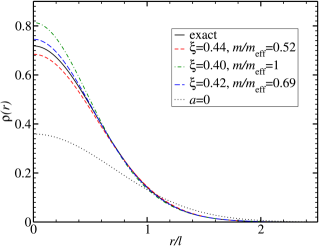
Figure 29: Papenbrock results from a density functional for the unitary regime.

Results of such fits are shown in Fig. 29. They predict $\xi=0.42$ and $m/m_{\rm eff}=0.69$ from the best fit. The value for $\xi$ is amazingly close to the Monte Carlo result. Papenbrock and Bhattacharyya Bhattacharyya:2006fg ; Papenbrock:2006hg consider corrections for an LDA density functional close to the unitary limit

$${\cal E}[\rho]={\cal E}_{\rm FG}\left(\xi+\frac{c_{1}}{a\rho^{1/3}}+c_{2}r_{0}\rho^{1/3}\right)\;.$$ (177)

Again, this is fit to the harmonically trapped two-fermion system. Results are given in Fig. 30 and show impressive agreement with Monte Carlo calculations.

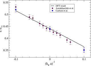
Figure 30: Papenbrock/Bhattacharyya DFT results for finite scattering length $a$ compared to Monte Carlo calculations.

Finally, there are interesting investigations of the constraints of general coordinate and conformal invariance by Dam Son and collaborators Son:2005rv ; Son:2005tj . They ask: Is there more than scale invariance for the unitary Fermi gas? The symmetries can be exposed by adding a background gauge field $A_{\mu}$ and curved space with metric $g_{ij}(t,{\bf x})$:

$$S\longrightarrow\int\!dt\,d{\bf x}\,\sqrt{g}\biggl{[}\frac{i}{2}\psi^{\dagger}\raisebox{1.00006pt}{$\stackrel{{\scriptstyle\scriptstyle\leftrightarrow}}{{\partial}}$}_{t}\psi-\frac{g^{ij}}{2m}(\partial_{i}+iA_{i})\psi^{\dagger}(\partial_{j}-iA_{j})\psi$$ (178)

$$\hskip 36.135pt\hbox{}+(q_{0}\sigma-A_{0})\psi^{\dagger}\psi-\frac{g^{ij}}{2}\partial_{i}\sigma\partial_{j}\sigma-\frac{\sigma^{2}}{2r_{0}^{2}}\biggr{]}\;.$$ (179)

This is more than scale and Galilean invariance! Direct consequences include extra constraints on ${\cal L}_{\rm eff}$ at NLO, which naively involve five arbitrary functions but these symmetries show there are only three. For the unitary Fermi gas, three constants from scale invariance are reduced to two constants from conformal invariance. This leads us to ask: What additional constraints can we find for the energy functional? This and the other open questions are ripe for investigation!

Acknowledgments: I thank the organizers of the Trento school, Janos Polonyi and Achim Schwenk, for the opportunity to participate in an excellent lecture series, and all the student participants, who made giving the lectures a pleasure. This work was supported in part by the National Science Foundation under Grant No. PHY–0354916 and the Department of Energy under Grant No. DE-FC02-07ER41457.

References

• (1) Recall that the wave function of a system of identical fermions must be antisymmetric under exchange of any two particles. This has important consequences for many-body systems, such as the development of a Fermi sea and “Pauli blocking”.
• (2) This figure was made by Jacek Dobaczewski.
• (3) M.A. Preson, R.K. Bhaduri: Structure of the Nucleus, (Addison-Wesley, Reading, MA, 1975)
• (4) A.D. Jackson: The Once and Future Nuclear Many-Body Problem. In: Recent Progress in Many-Body Theories, vol. 3, ed. T.L. Ainsworth, C.E. Campbell, B.E. Clements, E. Krotscheck (Plenum, New York, 1992)
• (5) A.D. Jackson, T. Wettig: Phys. Rep. 237, 325 (1994)
• (6) This figure was adapted by Achim Schwenk from a picture by A. Richter.
• (7) This discussion is adapted from a talk by Joe Carlson.
• (8) P. Ring, P. Schuck: The Nuclear Many-Body Problem (Springer, Berlin, 2005)
• (9) R.M. Dreizler, E.K.U. Gross: Density Functional Theory (Springer, Berlin 1990)
• (10) N. Argaman, G. Makov: Am. J. Phys. 68, 69 (2000)
• (11) A Primer in Density Functional Theory, eds. C. Fiolhais, F. Nogueira, M. Marques (Springer, Berlin, 2003)
• (12) The term “ab initio” is often used in this context, but the calculations do not in practice proceed only from the Coulomb interaction.
• (13) W. Koch, M. C. Holthausen: A Chemist’s Guide to Density Functional Theory (Wiley, New York 2000)
• (14) J.P. Perdew, S. Kurth, A. Zupan, P. Blaha: Phys. Rev. Lett. 82, 2544 (1999)
• (15) J. Polonyi, K. Sailer: Phys. Rev. B 66, 155113 (2002), [arXiv:cond-mat/0108179]
• (16) S.K. Bogner, A. Schwenk, R.J. Furnstahl, A. Nogga: Nucl. Phys. A763, 59 (2005)
• (17) R.B. Wiringa, V.G.J. Stoks, R. Schiavilla: Phys. Rev. C 51, 38 (1995)
• (18) D. Vautherin, D.M. Brink: Phys. Rev.  C 5, 626 (1972)
• (19) J. Dobaczewski, W. Nazarewicz, P.G. Reinhard: Nucl. Phys. A693, 361 (2001) [arXiv:nucl-th/0103001]
• (20) M. Bender, P. H. Heenen, P.-G. Reinhard: Rev. Mod. Phys.  75, 121 (2003)
• (21) A “local” potential is one whose action on a wavefunction in the Schrödinger equation is just $V({\bf r})\psi({\bf r})$; that is, it happens at one point. More generally, we expect something like $\int\!d{\bf r^{\prime}}\,V({\bf r},{\bf r^{\prime}})\psi({\bf r^{\prime}})$, which is not diagonal in coordinate representation. In momentum representation, this means $\langle{\bf k}|V|{\bf k^{\prime}}\rangle$ is not a function of ${\bf q}\equiv{\bf k}-{\bf k^{\prime}}$ only.
• (22) The goal of devising a potential that fits the scattering data as best as possible (that is, $\chi^{2}/\mbox{dof}\approx 1$) below where inelastic effects become important has been realized by several potentials, including CD-Bonn, Nijmegen I and II, and Argonne $v_{18}$.
• (23) Calculations of the energy of few-body nuclei using accurate two-body potentials have demonstrated the need for a three-body force.
• (24) All NN potentials have a cut-off on high-momentum (short-distance) contributions. Putting in a cut-off doesn’t mean the high-energy physics is thrown out, however! We need to renormalize (this is one of the main points of our discussion).
• (25) One way of specifying a many-body approximation is to say which Feynman diagrams are included. (If all are included, we’re solving the problem exactly!) Usually one needs to select an (infinite) subset (for example, the ladder or ring diagrams). In some case there are rigorous justifications for which to sum, but not always and there are seldom estimates available for what quantitative error is made by the truncation.
• (26) G.P. Lepage: What is Renormalization? In: From Actions to Answers (TASI-89), ed by T. DeGrand, D. Toussaint, (World Scientific, Singapore, 1989), p. 483
• (27) G.P. Lepage: How to Renormalize the Schrödinger Equation, Lectures given at 9th Jorge Andre Swieca Summer School: Particles and Fields, Sao Paulo, Brazil, February, 1997, arXiv:nucl-th/9706029
• (28) S.K. Bogner, R.J. Furnstahl: Phys. Lett. B 632, 501 (2006)
• (29) S.K. Bogner, R.J. Furnstahl: Phys. Lett. B 639, 237 (2006)
• (30) S.K. Bogner, T.T.S. Kuo, A. Schwenk, D.R. Entem, R. Machleidt: Phys. Lett. B 576, 265 (2003)
• (31) S.K. Bogner, T.T.S. Kuo, A. Schwenk: Phys. Rept. 386, 1 (2003)
• (32) S.K. Bogner, A. Schwenk, T.T.S. Kuo, G.E. Brown: arXiv:nucl-th/0111042
• (33) S.K. Bogner, R.J. Furnstahl, S. Ramanan, A. Schwenk, Nucl. Phys. A773, 203 (2006)
• (34) A.K. Kerman, J.P. Svenne, F.M.H. Villars: Phys. Rev. 147, 710 (1966)
• (35) W.H. Bassichis, A.K. Kerman, J.P. Svenne, Phys. Rev. 160, 746 (1967)
• (36) M.R. Strayer, W.H. Bassichis, A.K. Kerman: Phys. Rev. C 8, 1269 (1973)
• (37) A. Nogga, S.K. Bogner, A. Schwenk: Phys. Rev. C 70, 061002(R) (2004)
• (38) J.W. Negele, H. Orland: Quantum Many-Particle Systems (Addison-Wesley, New York 1988)
• (39) J. Zinn-Justin: Quantum Field Theory and Critical Phenomena 4th ed.  (Oxford University Press, New York 2002), ch. 12
• (40) For the Minkowski-space version of this discussion, see S. Weinberg: The Quantum Theory of Fields: vol. II, Modern Applications (Cambridge University Press 1996)
• (41) A. Schwenk, J. Polonyi: arXiv:nucl-th/0403011.
• (42) N. Nagaosa: Quantum Field Theory in Condensed Matter Physics (Springer Verlag, Berlin 1999)
• (43) M. Stone: The Physics of Quantum Fields (Springer Verlag, Berlin 2000)
• (44) R. Fukuda, M. Komachiya, S. Yokojima, Y. Suzuki, K. Okumura, T. Inagaki: Prog. Theor. Phys. Suppl.  121, 1 (1995)
• (45) M. Valiev, G.W. Fernando: arXiv:cond-mat/9702247
• (46) M. Valiev, G.W. Fernando: Phys. Lett. A 227, 265 (1997)
• (47) M. Rasamny, M.M. Valiev, G.W. Fernando: Phys. Rev. B 58, 9700 (1998)
• (48) To derive the second equality for $f_{l}(k)$, first put the $e^{i\delta_{l}}$ in the denominator, then replace it by $\cos+i\sin$ and divide top and bottom by $\sin$.
• (49) H.W. Hammer, R.J. Furnstahl: Nucl. Phys. A678, 277 (2000)
• (50) S.R. Beane, P.F. Bedaque, W.C. Haxton, D.R. Phillips, M.J. Savage: arXiv:nucl-th/0008064
• (51) E. Braaten, A. Nieto: Phys. Rev. B 55, 8090 (1997); 56, 14745 (1997)
• (52) S.J. Puglia, A. Bhattacharyya, R.J. Furnstahl: Nucl. Phys. A 723, 145 (2003) [arXiv:nucl-th/0212071]
• (53) A. Bhattacharyya, R.J. Furnstahl: Nucl. Phys. A 747, 268 (2005) [arXiv:nucl-th/0408014]
• (54) A. Bhattacharyya, R.J. Furnstahl: Phys. Lett. B 607, 259 (2005) [arXiv:nucl-th/0410105]
• (55) R.J. Bartlett, V.F. Lotrich, I.V. Schweigert: J. Chem. Phys. 123, 062205 (2005)
• (56) A. Görling, J. Chem. Phys. 123, 062203 (2005)
• (57) E.J. Baerends, O.V. Gritsenko: J. Chem. Phys. 123, 062202 (2005)
• (58) R.J. Furnstahl, H.W. Hammer: Phys. Lett.  B 531, 203 (2002) [arXiv:nucl-th/0108069]
• (59) A. Bulgac: Phys. Rev. C 65, 051305 (2002) [arXiv:nucl-th/0108014]
• (60) A. Bulgac, Y. Yu: Phys. Rev. Lett.  88, 042504 (2002) [arXiv:nucl-th/0106062]
• (61) Y. Yu, A. Bulgac: Phys. Rev. Lett.  90, 222501 (2003) [arXiv:nucl-th/0210047]
• (62) L.N. Oliveira, E.K.U. Gross, W. Kohn: Phys. Rev. Lett. 60, 2430 (1988)
• (63) S. Kurth, M. Marques, M. Lüders, E.K.U. Gross,: Phys. Rev. Lett. 83, 2628 (1999)
• (64) R.J. Furnstahl, H.W. Hammer, S.J. Puglia: arXiv:nucl-th/0612086
• (65) T. Papenbrock, G.F. Bertsch: Phys. Rev. C 59, 2052 (1999)
• (66) L.P. Gor’kov, T.K. Melik-Barkhudarov: Sov. Phys. JETP 13, 1018 (1961)
• (67) H. Heiselberg, C.J. Pethick, H. Smith, L. Viverit: Phys. Rev. Lett. 85, 2418 (2000)
• (68) R.J. Furnstahl: J. Phys. G 31, S1357 (2005) [arXiv:nucl-th/0412093]
• (69) D.R. Entem, R. Machleidt: Phys. Rev. C 68, 041001(R) (2003)
• (70) E. Epelbaum, W. Glöckle, U.G. Meißner: Nucl. Phys. A747, 362 (2005)
• (71) S.K. Bogner, R.J. Furnstahl, R.J. Perry: arXiv:nucl-th/0611045
• (72) S.K. Bogner, R.J. Furnstahl, R.J. Perry, A. Schwenk: arXiv:nucl-th/0701013
• (73) L. Coraggio, A. Covello, A. Gargano, N. Itaco, D.R. Entem, T.T.S. Kuo, R.Machleidt: arXiv:nucl-th/0701065
• (74) J.W. Negele, D. Vautherin: Phys. Rev. C 5, 1472 (1972)
• (75) J.W. Negele, D. Vautherin: Phys. Rev. C 11, 1031 (1975)
• (76) S.K. Bogner, R.J. Furnstahl, L. Platter: in preparation
• (77) N. Kaiser, S. Fritsch, W. Weise: Nucl. Phys. A 724, 47 (2003)
• (78) N. Kaiser: Phys. Rev. C 68, 014323 (2003)
• (79) N. Kaiser et al.: Nucl. Phys. A750, 259 (2005)
• (80) V. Rotivale, S.K. Bogner, T. Duguet, R.J. Furnstahl: in preparation
• (81) J. Engel: arXiv:nucl-th/0610043
• (82) B.D. Serot, J.D. Walecka: Adv. Nucl. Phys. 16, 1 (1986)
• (83) P. Ring: Prog. Part. Nucl. Phys. 37, 193 (1996), and references therein
• (84) B.D. Serot, J.D. Walecka: Int. J. Mod. Phys. E 6, 515 (1997), and references therein
• (85) J. Gasser, M.E. Sainio, A. Svarc: Nucl. Phys. B307, 779 (1988)
• (86) E. Jenkins, A.V. Manohar: Phys. Lett. B 255, 558 (1991);
V. Bernard, N. Kaiser, U.-G. Meissner: Nucl. Phys. B388, 315 (1992)
• (87) H.-B. Tang: arXiv:hep-ph/9607436
• (88) P.J. Ellis, H.-B. Tang: Phys. Rev. C 57, 643 (1998)
• (89) T. Becher, H. Leutwyler: Eur. Phys. J. C9, 643 (1999)
• (90) T. Fuchs et al: arXiv:hep-ph/0302117
• (91) D. Lehmann, G. Prezeau: Phys. Rev. D 65, 016001 (2002)
• (92) M.R. Schindler, J. Gegelia, S. Scherer: Phys. Lett.  B 586, 258 (2004) [arXiv:hep-ph/0309005]
• (93) D.B. Kaplan, M.J. Savage, M.B. Wise: Phys. Lett. B 424, 390 (1998); Nucl. Phys. B 534, 329 (1998)
• (94) S. Y. Chang et al.: Nucl. Phys.  A 746, 215 (2004) [arXiv:nucl-th/0401016]
• (95) G.E. Astrakharchik, J. Boronat, J. Casulleras, S. Giorgini Phys. Rev. Lett. 93, 200404 (2004)
• (96) T. Papenbrock: Phys. Rev.  A 72, 041603 (2005) [arXiv:cond-mat/0507183]
• (97) A. Bhattacharyya, T. Papenbrock: arXiv:nucl-th/0602050
• (98) T. Papenbrock, A. Bhattacharyya: Phys. Rev.  C 75, 014304 (2007) [arXiv:nucl-th/0609084].
• (99) D. T. Son, M. Wingate: Annals Phys.  321, 197 (2006) [arXiv:cond-mat/0509786]
• (100) D. T. Son: Phys. Rev. Lett.  98, 020604 (2007) [arXiv:cond-mat/0511721]
Index