Di-electrons from $\eta$ meson Dalitz decay in proton-proton collisions

Abstract

The reaction $pp\to pp\eta\to pp\gamma e^{+}e^{-}$ is discussed within a covariant effective meson-nucleon theory. The model is adjusted to data of the subreaction $pp\to pp\eta$. Our focus is on di-electrons from Dalitz decays of $\eta$ mesons, $\eta\to\gamma\gamma^{*}\to\gamma e^{+}e^{-}$, and the role of the corresponding transition form factor $F_{\eta\gamma\gamma^{*}}$. Numerical results are presented for the intermediate energy kinematics of HADES experiments.

I Introduction

The $\eta$ meson as member of the octet of Goldstone bosons has the valence quark structure $(\bar{u}u+\bar{d}d-\bar{s}s)/\sqrt{3}$ when choosing the mixing angle of 19.5^o in superimposing the octet-$\eta_{8}$ and singlet-$\eta_{0}$. Various conservations laws forbid low-order decays causing the very narrow $\eta$ width. This makes the $\eta$ decays sensitive for testing invariances of the standard model. The hidden strangeness content lets one argue for some sensitivity to the strangeness content of the nucleon when considering $\eta$ production off nucleons. Consequently, the $\eta$ production and various special decay channels were subject of intense investigations since some time, both experimentally and theoretically.

There is a rich data basis for $\eta$ production in nucleon-nucleon collisions providing a test ground for meson production in strong interaction processes, in particular near threshold. Due to the iso-scalar character of the $\eta$ meson, $\eta$ production off the nucleon proceeds via selected baryon resonances thus allowing differential access to resonance properties.

Furthermore, the Dalitz decay $\eta\to\gamma e^{+}e^{-}$ constitutes a prominent source of di-electrons in intermediate-energy heavy-ion collisions. Indeed, the recent HADES data HADES_PRL exhibit a sizeable yield of $e^{+}e^{-}$ in the invariant-mass region 150 - 500 MeV which is essentially attributed HW_HADES to $\eta$ Dalitz decays, but $\Delta$ Dalitz decays and non-resonant virtual bremsstrahlung ourNuclPhys contribute in this region, too. The primary aim of the HADES experiments HADES is to seek for signals of chiral symmetry restoration in compressed nuclear matter. For such an enterprize one needs good control of the competing background processes, among them the mentioned $\eta$ Dalitz decays.

$\eta$ Dalitz decays depend on the pseudo-scalar transition form factor. Such form factors encode information on hadrons which is accessible in first-principle QCD calculations or abridged variants thereof, such as effective hadron theories or QCD sum rules. In so far, experimental information on transition form factors is quite valuable LandPhysRep . Given this motivation we consider here the process of Dalitz decay of the pseudo-scalar $\eta$ meson

$$\eta\to\gamma+\gamma^{*}\to\gamma+e^{-}+e^{+},$$ (1)

where $\gamma^{*}$ denotes a virtual photon. Obviously, the probability of emitting a virtual photon is governed by the dynamical electromagnetic structure of the dressed transition vertex $\eta\to\gamma\gamma^{*}$ which is condensed in the transition form factor $F_{\eta\gamma\gamma^{*}}$. If the decaying hadron were point like, then a calculation of mass distributions and decay widths would be straightforward along the standard quantum electrodynamics (QED). Deviations of the measured quantities from QED predictions directly reflect the effects of the form factor and thus the internal hadron structure.

Often, the production process and the decay process are dealt with separately. With respect to available new data from HADES hadeseta the reaction

$$p_{1}+p_{2}\to p_{1}^{\prime}+p_{2}^{\prime}+\eta\to p_{1}^{\prime}+p_{2}^{\prime}+\gamma+e^{+}+e^{-},$$ (2)

which will be improved in near future, we consider the complete reaction (2) in which (1) figures as a subreaction. The employed framework is that of an effective description in a hadronic basis. To be specific, we are going to parameterize the $\eta$ production subreaction in nucleon-nucleon ($NN$) collisions within the one-boson exchange (OBE) model. Such an approach has been utilized fairly successfully by various authors in the past. For instance, in Ref. wilkinEta a model based on OBE with nucleons only has been facilitated for $pp\to pp\eta$ and $pd\to pd\eta$ reactions. A non-relativistic approach was proposed in Ref. santraEta . In gedalinEta a description based on OBE without internal meson conversion and with the resonance $S_{11}(1535)$ has been elaborated for $NN\to NN\eta$ in a region sufficiently above the threshold. A detailed analysis of $NN\to NN\eta$ has been worked out by Nakayama and collaborators nakayamaEta . For a study of the role of nucleon resonances in $\eta$ photo-production we refer the interested reader to Ref. moselEta .

In contrast to a factorized description with production of an on-shell $\eta$ and an independent decay of an on-shell $\eta$ we attempt here a complete description of the whole reaction (2). That means we supplement the subreaction $NN\to NN\eta$ by the Dalitz decay part thus dealing with intermediate off-shell $\eta$ meson. This allows considering di-electron masses larger than the pole-mass of the $\eta$ meson (for the on-shell $\eta$ meson the invariant mass of the di-electron is restricted by the mass of the $\eta$ meson). This can furnish additional information on the transition form factor in a larger kinematical region.

Our paper is organized as follows. In section 2 we introduce the $\eta\to\gamma\gamma^{*}$ transition form factor. Section 3 is devoted to the theoretical background for dealing with the reaction $pp\to pp\eta\to pp\gamma e^{+}e^{-}$. It is essentially based on an extension of the effective model ourOmega ; ourPhi adjusted to vector (V) meson production in $NN\to NNV$ reactions. The model utilizes a direct calculations of the relevant tree-level Feynman diagrams within a phenomenological meson-nucleon theory. The model parameters have been previously fixed from independent experiments and adjusted to achieve a good description the available experimental data ourOmega ; ourPhi . However, in the present paper also diagrams with excitation of nucleon resonances with masses close to the mass of a nucleon plus $\eta$ meson are included. These are $S_{11}(1535)$ , $D_{13}(1520)$ and $P_{11}(1440)$ resonances. The corresponding effective constants, whenever possible, are obtained from the known decay widths of direct decay into $\eta$ channel or radiative decay with subsequent use of vector meson dominance. We use effective constants commonly adopted in the literature and obtained from different considerations, e.g., SU(3) symmetry or adjustment to photoabsorbtion etc. nakayamaEta . Numerical results are presented in section 4, where we consider separately the reaction $NN\to NN\eta$. Results for the full reaction (2) are described in section 5 with emphasis on the role of the $\eta\gamma\gamma^{*}$ transition form factor. The conclusions are summarized in section 6, and some formal relations are relegated to the appendices.

II Dalitz decay and Transition Form Factor

Let us first consider first the process of a two-photon decay of an $\eta$ meson. The effective Lagrangian describing the vertex $\eta\to\gamma\gamma$ reads meissner ; thomas ; anisovich_FF ; faessler

$${\cal L}_{\eta\gamma\gamma}=f_{\eta\gamma\gamma}\ \left(\epsilon_{\mu\nu\alpha\beta}\partial^{\mu}A^{\nu}\partial^{\alpha}A^{\beta}\right)\Phi_{\eta},$$ (3)

where $A^{\nu}$ is the electromagnetic four-potential, $\Phi_{\eta}$ denotes the pseudo-scalar $\eta$ meson field and $f_{\eta\gamma\gamma\,}$ is the corresponding coupling constant. The fully antisymmetric Levi-Civita symbol $\epsilon_{\mu\nu\alpha\beta}$ is normalized as $\epsilon_{0123}=-1$. The $\eta$ decay width follows from (3) as

$$\Gamma_{\eta\to\gamma\gamma}=\frac{s_{\eta}^{3/2}}{64\pi}f_{\eta\gamma\gamma}^{2}$$ (4)

and serves for a determination of the coupling constant $f_{\eta\gamma\gamma}$ from experimental data. The square of the $\gamma\gamma$ invariant mass is denoted by $s_{\eta}$, $s_{\eta}=m_{\eta}^{2}$ for an on-shell $\eta$ meson. (Note that contrarily to the vector meson case ourFF , instead of a factor $1/3$ [due to averaging over three projections of the spin of the vector particle] in eq. (4) a factor of $1/2$ appears due to two photons in the final state.) Experimentally, the branching ratio $Br(\eta\to\gamma\gamma)=\Gamma_{\eta\to\gamma\gamma}/\Gamma_{\eta,tot}$ is known as $\left(39.38\pm 0.26\right)$% dataGroup . Eq. (4) yields $|f_{\eta\gamma\gamma\,}|\simeq 0.025\,GeV^{-1}$ for the known total width $\Gamma_{\eta,tot}=(1.3\pm 0.07)\,keV$. Since in our further calculations the cross section is directly proportional to $|f_{\eta\gamma\gamma\,}|^{2}$, the sign of the coupling constant does not play a role and for definiteness it has been taken positively.

In the decay (1), however, one of the emitted photons is virtual with a time-like four-momentum and, consequently, the Lagrangian (3) must be supplemented by inclusion of the corresponding transition form factor (FF). We employ the following procedure:

$$f_{\eta\gamma\gamma}(0)\to f_{\eta\gamma\gamma^{*}}(s_{\gamma^{*}})=f_{\eta\gamma\gamma}(0)\,F_{\eta\gamma{\gamma^{*}}}(s_{\gamma^{*}})$$ (5)

where $s_{\gamma^{*}}$ is the di-electron invariant mass squared and $f_{\eta\gamma\gamma}(0)\equiv|f_{\eta\gamma\gamma}|$. Formally, eq. (5) can be considered as the definition of the transition form factor. By a direct calculation of the corresponding diagram for the decay rate $d\Gamma/ds_{\gamma^{*}}$ for the $\eta$ meson one finds LandPhysRep

$$\displaystyle\frac{d\Gamma_{\eta\to\gamma e^{+}e^{-}}}{ds_{\gamma^{*}}}=\displaystyle\frac{2\alpha}{3\pi s_{\gamma^{*}}}\left(1-\frac{s_{\gamma^{*}}}{m_{\eta}^{2}}\right)^{3}\left(1-\frac{4\mu_{e}^{2}}{s_{\gamma^{*}}}\right)^{1/2}\left(1+2\frac{\mu_{e}}{s_{\gamma^{*}}}\right)\Gamma_{\eta\to\gamma\gamma}\left|F_{\eta\gamma\gamma^{*}\,}(s_{\gamma^{*}})\right|^{2}$$ (6)

with $\alpha$ as electromagnetic fine structure constant and $\mu_{e}$ the electron mass. In the kinematical region we are interested in the terms with $\mu_{e}$ can be neglected. Putting $\left|F_{\eta\gamma\gamma^{*}\,}(s_{\gamma^{*}})\right|^{2}=1$ would mean neglecting the finite size and internal structure of $\eta$. It is seen that the differential decay width $d\Gamma_{\eta\to\gamma e^{+}e^{-}}/ds_{\gamma^{*}}$ is determined by (i) a purely kinematical (calculable) factor, (ii) the real photon decay vertex $\eta\to\gamma\gamma$ (known from experimental data), and (iii) the (wanted) transition FF $F_{\eta\gamma\gamma^{*}\,}(s_{\gamma^{*}})$. Hence, eq. (6) evidences that by measuring the invariant mass distribution one can get direct experimental access to the transition FF LandPhysRep ; omegaFrmf1 ; omegaFrmf2 ; omegaFrmf3 . For a on-mass shell $\eta$ meson, the value of the di-electron mass $s_{\gamma^{*}}$ is kinematically restricted by $s_{\gamma^{*}}\leq m_{\eta}^{2}$. In case of reactions of the type (2) the intermediate $\eta$ meson can be off-shell and, in principle, the value of the di-electron invariant mass can be larger than the $\eta$ pole mass. This situation will be investigated below.

A quite successful theoretical approach to FF’s is based on the vector meson dominance (VMD) conjecture faessler ; meissner . Reasonably good descriptions of elastic FF’s in the time-like region has been accomplished, indeed. By using the current-field identity meissner

$$J^{\mu}=-e\frac{M_{\rho}^{2}}{f_{\gamma\rho}}\Phi_{\rho^{0}}^{\mu}-e\frac{M_{\omega}^{2}}{f_{\gamma\omega}}\Phi_{\omega}^{\mu}$$ (7)

with coupling constants $f_{\gamma\rho}$ and $f_{\gamma\omega}$ known friman1 ; friman2 from experimentally measured electromagnetic decay widths, one can also compute the transition form factor $F^{VMD}_{\eta\gamma\gamma^{*}\,}(s_{\gamma^{*}})$ by evaluating the corresponding Feynman diagrams (see below). Contrary to the transition FF of vector meson production ourFF , the $\eta$ meson FF, computed within such an approach, exhibits a rather good agreement with previous data LandPhysRep ; omegaFrmf1 ; omegaFrmf2 ; omegaFrmf3 .

III Model

We implement the discussed Dalitz decay $\eta\to\gamma e^{+}e^{-}$ into a more general process of di-electron production in $NN$ reactions with intermediate $\eta$. Consider the reaction (2) for which the process (1) enters as a subreaction. The invariant cross section is

$$d^{11}\sigma=\frac{1}{2\sqrt{\lambda(s,m_{N}^{2},m_{N}^{2})}}\frac{1}{(2\pi)^{11}}\frac{1}{4}\sum\limits_{\rm spins}\ \,|\ T(P_{1}^{\prime},P_{2}^{\prime},k_{1},k_{2},k_{\pi},{\rm spins})\ |^{2}d^{11}\tau_{f}\ \frac{1}{n!},$$ (8)

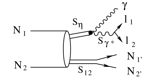
Figure 1: Illustration of the choice of the independent variables for the process $N_{1}+N_{2}\to N_{1}^{\prime}+N_{2}^{\prime}+\gamma+l_{1}+l_{2}$ ($l_{1}=e^{+}$, $l_{2}=e^{-}$) within the duplication kinematics bykling . The invariant mass squared of the two final nucleons is denoted by $s_{12}$, while the invariant mass of the subsystem $\gamma e^{+}e^{-}$ is $s_{\eta}$.

where the factor $1/n!$ accounts for $n$ identical particles in the final state, $|T|^{2}$ denotes the invariant amplitude squared and $d\tau_{f}$ is the invariant phase volume which is chosen within the so-called ”duplication” kinematics bykling , i.e. the one which exploits invariant two-dimensional phase volumes $R_{2}$ describing the decay kinematics of a real or virtual particle with the invariant mass squared $s$ ($s>0$) into two particles, which can also be either real or virtual. This kinematics is schematically depicted in Fig. 1. Such a choice of kinematical variables is extremely useful if one considers specific classes of Feynman diagrams which allow to separate some vertices in a factorized form. Then in the total cross section some integrations can be performed analytically (see ourNuclPhys ; ourFF ). For the present task we need to consider only such types of diagrams which allows to factorize the meson decay vertex from the parts describing the creation of the meson in a $NN$ interaction. Consequently, analytical integrations can be executed over the variables connected with the decay vertex.

III.1 Nucleon Current

The invariant amplitude $T$ is evaluated here within a phenomenological meson-nucleon theory based on effective interaction Lagrangians which include scalar ($\sigma$), pseudo-scalar isovector ($\pi$), neutral pseudo-scalar ($\eta$) and neutral vector ($\omega$) and vector isovector ($\rho$) mesons (see nakayamaEta ; ourPhi ; ourOmega ; ourNuclPhys )

$${\cal L}_{\sigma NN} = g_{\sigma NN}\bar{N}N\it\Phi_{\sigma},$$ (9)

$${\cal L}_{\pi NN} = -\frac{f_{\pi NN}}{m_{\pi}}\bar{N}\gamma_{5}\gamma^{\mu}\partial_{\mu}({{\mathchar 28956\relax}{\mathchar 28680\relax}_{\pi}})N,$$ (10)

$${\cal L}_{\eta NN} = -\frac{f_{\eta NN}}{m_{\eta}}\bar{N}\gamma_{5}\gamma^{\mu}\partial_{\mu}\Phi_{\eta}N,$$ (11)

$${\cal L}_{\rho NN} = -g_{\rho NN}\left(\bar{N}\gamma_{\mu}{{\mathchar 28956\relax}}N{{\mathchar 28680\relax}_{\rho}}^{\mu}-\frac{\kappa_{\rho}}{2m_{N}}\bar{N}\sigma_{\mu\nu}{{\mathchar 28956\relax}}N\partial^{\nu}{{\mathchar 28680\relax}_{\rho}}^{\mu}\right),$$ (12)

$${\cal L}_{\omega NN} = -g_{\omega NN}\left(\bar{N}\gamma_{\mu}N{\it\Phi}_{\omega}^{\mu}-\frac{\kappa_{\omega}}{2m_{N}}\bar{N}\sigma_{\mu\nu}N\partial^{\nu}\it\Phi_{\omega}^{\mu}\right),$$ (13)

where $N$ and $\it\Phi$ denote the nucleon and meson fields, respectively and bold face letters stand for isovectors. All couplings with off-mass shell mesons are dressed by monopole form factors $F_{M}=\left(\Lambda^{2}_{M}-\mu_{M}^{2}\right)/\left(\Lambda^{2}_{M}-k^{2}_{M}\right)$, where $k^{2}_{M}$ is the four-momentum of a virtual meson with mass $\mu_{M}$.

The Lagrangians (9 - 13) are needed in evaluations of Feynman diagrams describing the Dalitz decay of the $\eta$ meson created from nucleon bremsstrahlung due to $NN$ interaction via one-boson exchange, see Fig. 2a.

III.2 Internal Conversion Current

The $\eta$ meson can also be produced by an internal conversion of the exchanged mesons, the so-called conversion current. The dominant exchange vector mesons ($V$) in this case are $\omega$ and $\rho$ mesons with the interaction Lagrangians

$${\cal L}_{\eta\omega\omega} = -\frac{g_{\eta\omega\omega}}{2m_{\omega}}\,\varepsilon_{\mu\nu\alpha\beta}\,\left(\partial^{\mu}\it\Phi_{\omega}^{\nu}\partial^{\alpha}\it\Phi_{\omega}^{\beta}\right)\Phi_{\eta},$$ (14)

$${\cal L}_{\eta\rho\rho} = -\frac{g_{\eta\rho\rho}}{2m_{\rho}}\,\varepsilon_{\mu\nu\alpha\beta}\,\left(\partial^{\mu}\it{\mathchar 28680\relax}_{\rho}^{\nu}\partial^{\alpha}\it{\mathchar 28680\relax}_{\rho}^{\beta}\right)\Phi_{\eta}.$$ (15)

The corresponding diagrams are exhibited in Fig. 2b.

The $VV\eta$ vertices in the conversion diagrams have been calculated from the radiative decay $V\to\eta\gamma$ within the VMD model nakayamaEta ; durso . Correspondingly, the vertex form factor $VV\eta$ is chosen as

$$F_{VV\eta}(\Lambda,k_{1}^{2},k_{2}^{2})=\frac{\Lambda^{2}-m_{V}^{2}}{\Lambda^{2}-k_{1}^{2}}\frac{\Lambda^{2}}{\Lambda^{2}-k_{2}^{2}}$$ (16)

which, in accordance with the procedure of determining the coupling constant, is normalized to unity when one vector meson is on-mass shell and the other one becomes massless, e.g., $F_{VV\eta}(\Lambda,k_{1}^{2}=m_{V}^{2},k_{2}^{2}=0)=1$.

III.3 Nucleon Resonance Current

In the threshold-near kinematics for $\eta$ production in $NN$ reactions there are a few nucleon resonances with masses $m_{N^{*}}\sim m_{N}+m_{\eta}$ which can contribute to the cross section. These are $S_{11}(1535)$ and $D_{13}(1520)$ with odd parity and spins $\frac{1}{2}$ and $\frac{3}{2}$, respectively, and the spin-$\frac{1}{2}$ even-parity $P_{11}(1440)$ Roper resonance with nucleon quantum numbers. The corresponding interaction Lagrangians for $S_{11}(1535)$ are nimaiResonances ; nakayamaEta

$${\cal L}_{\eta NN_{1535}} = \frac{g_{\eta NN_{1535}}}{m_{N^{*}}-m_{N}}\bar{N}^{*}\gamma_{\mu}\partial^{\mu}\Phi_{\eta}N+h.c.,$$ (17)

$${\cal L}_{\pi NN_{1535}} = \frac{g_{\pi NN_{1535}}}{m_{N^{*}}-m_{N}}\bar{N}^{*}\gamma_{\mu}\partial^{\mu}{\mathchar 28956\relax}{\mathchar 28680\relax}_{\pi}N+h.c.,$$ (18)

$${\cal L}_{\omega NN_{1535}} = \frac{g_{\omega NN_{1535}}}{m_{N^{*}}+m_{N}}\bar{N}^{*}\gamma_{5}\sigma_{\mu\nu}\partial^{\nu}\Phi^{\mu}_{\omega}N+h.c.,$$ (19)

$${\cal L}_{\rho NN_{1535}} = \frac{g_{\rho NN_{1535}}}{m_{N^{*}}+m_{N}}\bar{N}^{*}\gamma_{5}\sigma_{\mu\nu}\partial^{\nu}{\mathchar 28956\relax}{\mathchar 28680\relax}^{\mu}_{\rho}N+h.c..$$ (20)

For the spin-$\frac{3}{2}$ resonance $D_{13}(1520)$ we employ

$${\cal L}_{\eta NN_{1520}} = \frac{g_{\eta NN_{1520}}}{m_{\eta}}\bar{N}^{*\mu}\Theta_{\mu\nu}(z)\gamma_{5}\partial^{\nu}\Phi_{\eta}N+h.c.,$$ (21)

$${\cal L}_{\pi NN_{1520}} = \frac{g_{\pi NN_{1520}}}{m_{\pi}}\bar{N}^{*\mu}\Theta_{\mu\nu}(z)\gamma_{5}\partial^{\nu}{\mathchar 28956\relax}{\mathchar 28680\relax}_{\pi}N+h.c.,$$ (22)

$${\cal L}_{\omega NN_{1520}} = i\frac{g^{(1)}_{\omega NN_{1520}}}{2m_{N}}\bar{N}^{*\mu}\Theta_{\mu\nu}(z)\gamma_{\alpha}\omega^{\alpha\nu}N\,-\,\frac{g^{(2)}_{\omega NN_{1520}}}{4m_{N}^{2}}\partial_{\alpha}\bar{N}^{*\mu}\omega^{\alpha\mu}N+h.c.,$$ (23)

$${\cal L}_{\rho NN_{1520}} = i\frac{g^{(1)}_{\rho NN_{1520}}}{2m_{N}}\bar{N}^{*\mu}\Theta_{\mu\nu}(z)\gamma_{\alpha}{\mathchar 28956\relax}{\mathchar 28954\relax}^{\alpha\nu}N\,-\,\frac{g^{(2)}_{\rho NN_{1520}}}{4m_{N}^{2}}\partial_{\alpha}\bar{N}^{*\mu}{\mathchar 28956\relax}{\mathchar 28954\relax}^{\alpha\nu}N+h.c.,$$ (24)

where $\Theta_{\mu\nu}(z)=g_{\mu\nu}-(A(1+4z)/2+z)\gamma_{\mu}\gamma_{\nu}$. The field strengths $\omega^{\alpha\mu}$ and ${\mathchar 28954\relax}^{\alpha\nu}$ are $\omega^{\alpha\mu}(x)=\partial^{\alpha}\Phi_{\omega}^{\mu}(x)-\partial^{\mu}\Phi_{\omega}^{\alpha}(x)$ and ${\mathchar 28954\relax}^{\alpha\nu}(x)=\partial^{\alpha}{\mathchar 28680\relax}_{\rho}^{\mu}(x)-\partial^{\mu}{\mathchar 28680\relax}_{\rho}^{\alpha}(x)$, respectively. The interactions (21 - 24) with $\Theta_{\mu\nu}(z)$ have been extensively discussed in the literature (see, e.g., Ref. davitsonDelta and further references quoted therein). The form of $\Theta_{\mu\nu}(z)$ is chosen in such a way that the respective interaction Lagrangian obeys the same point transformation as the free Lagrangian, which ensures that the matrix elements are independent of the parameter $A$, usually taken as $A=-1$. The off-shell parameter $z$ remains free thereby. We employ here $z=-1/2$. Also, the choice of the form of higher spin $\bar{s}\geq\frac{3}{2}$ propagators has been a subject of discussion in the literature ourNuclPhys ; prop4 ; prop5 ; prop6 ; prop7 , e.g., with concerns about the spin-projector operator ${\cal P}_{\frac{3}{2}}$ (off-mass shell vs. on-shell) or the ordering of the product of energy projection operator $\hat{P}_{N^{*}}+m_{N^{*}}$ and ${\cal P}_{\frac{3}{2}}$ (only on the mass shell these two operators commute). In the present paper we take the spin-$\frac{3}{2}$ propagator in the form ourNuclPhys

$$S_{\frac{3}{2}}^{\mu\nu}(P) = -i\frac{\hat{P}_{N^{*}}+m_{N^{*}}}{P^{2}-m_{N^{*}}^{2}}{\cal P}_{\frac{3}{2}}^{\mu\nu}(P),$$ (25)

where the spin projection operator is of the form

$${\cal P}_{\frac{3}{2}}^{\mu\nu}(P) = g^{\mu\nu}-\frac{1}{3}\gamma^{\mu}\gamma^{\nu}-\frac{2P^{\mu}P^{\nu}}{3m_{N^{*}}^{2}}-\frac{1}{3m_{N^{*}}}\left(\gamma^{\mu}P^{\nu}-\gamma^{\nu}P^{\mu}\right),$$ (26)

as commonly adopted within the Rarita-Schwinger formalism fron .

For $P_{11}(1440)$ the effective Lagrangians are similar to that for $S_{11}$, except for the relative signs in $\eta$ and $\pi$ couplings and the $\sigma NN^{*}$ Lagrangian, i.e.

$${\cal L}_{\eta NN_{1440}} = -\frac{g_{\eta NN_{1440}}}{m_{N^{*}}+m_{N}}\bar{N}^{*}\gamma_{5}\gamma_{\mu}\partial^{\mu}\Phi_{\eta}N+h.c.,$$ (27)

$${\cal L}_{\pi NN_{1440}} = -\frac{g_{\pi NN_{1535}}}{m_{N^{*}}+m_{N}}\bar{N}^{*}\gamma_{5}\gamma_{\mu}\partial^{\mu}{\mathchar 28956\relax}{\mathchar 28680\relax}_{\pi}N+h.c.,$$ (28)

$${\cal L}_{\sigma NN_{1440}} = g_{\sigma NN_{1440}}\bar{N}^{*}N\it\Phi_{\sigma}+h.c.,$$ (29)

$${\cal L}_{\omega NN_{1440}} = \frac{g_{\omega NN_{1440}}}{m_{N^{*}}+m_{N}}\bar{N}^{*}\sigma_{\mu\nu}\partial^{\nu}\Phi^{\mu}_{\omega}N+h.c.,$$ (30)

$${\cal L}_{\rho NN_{1440}} = \frac{g_{\rho NN_{1440}}}{m_{N^{*}}+m_{N}}\bar{N}^{*}\sigma_{\mu\nu}\partial^{\nu}{\mathchar 28956\relax}{\mathchar 28680\relax}^{\mu}_{\rho}N+h.c..$$ (31)

These interaction Lagrangians enter the nucleon resonance current exhibited in Fig. 2a.

In order to account for the finiteness of the resonance widths $\Gamma$, the resonance mass in the corresponding propagators is augmented by an imaginary part, $m_{N^{*}}\to m_{N^{*}}-i\Gamma_{N^{*}}/2$. Also for the resonance and conversion currents all the vertices with off-shell hadrons are dressed by form factors

$$F(\Lambda,p^{2})=\frac{\Lambda^{4}}{\Lambda^{4}+(p^{2}-m^{2})^{2}}.$$ (32)

III.4 Effective parameters

The effective parameters of the Lagrangians (9 - 13) which determine the pure nucleon current diagrams are basically the ones from the OBE Bonn potential bonncd which have been used in our previous calculations for vector meson ($\omega$, $\rho$ and $\phi$) production in $NN$ interactions ourOmega ; ourFF , see Tab. 1. The nucleon cut-off parameter for the bremsstrahlung $NN\eta$ vertex is $\Lambda^{br.}_{\eta NN}=1.2\,GeV$.

Table 1: Coupling constants and cut-off parameters for the nucleon current bonncd .

		$g_{MNN}$		$\Lambda_{MNN}\,[GeV]$
$\pi$		$f_{\pi NN}=1.0$		$1.3$
$\eta$		$f_{\eta NN}=1.79$		$1.8$
$\sigma$		$g_{\sigma NN}=10.$		$1.8$
$\rho$		$g_{\rho NN}=3.5$		$1.3$
		($\kappa_{\rho}=6.1$)
$\omega$		$g_{\omega NN}=15.85$		$1.5$
		($\kappa_{\omega}=0.0$)

The effective coupling constants for the nucleon resonance currents, whenever possible, have been obtained from the known decay widths of direct decay into $\eta$ channels or radiative decay with subsequent use of VMD. Otherwise, we use effective constants commonly utilized in the literature and obtained from different considerations, e.g., SU(3) symmetry, fit of photo-absorbtion reactions etc. (see, e.g. nakayamaEta ). The few remaining less known cut-off parameters are taken either close to the ones from OBE potential (for instance, the $\Lambda_{\rho NN^{*}}$ and $\Lambda_{\omega NN^{*}}$ cut off’s are chosen equal to $\Lambda_{\omega NN}=1.5\,GeV$; $\Lambda_{\eta NN_{1535}}=\Lambda_{\eta NN_{1440}}=\Lambda_{\eta NN}=1.3\,GeV$, cf. Tab. 2) or adjusted to experimental data (see below). The resonance cut-off parameters for the bremsstrahlung $N^{*}N\eta$ vertex have been taken as $\Lambda^{br.}_{\eta NN_{1535}}=1.3\,GeV$, $\Lambda^{br.}_{\eta NN_{1520}}=1.1\,GeV$ and $\Lambda^{br.}_{\eta NN_{1440}}=1.2\,GeV$, respectively.

Table 2: Coupling constants and cut-off parameters for the nucleon resonance current. For the spin-$\frac{3}{2}$ resonance $D_{13}$ the off-shell parameter $z=-1/2$ is used and the second coupling constant, eq. (24), with vector mesons is given in parenthesis. For a reasoning of $g_{\pi NN^{*}}$ and $g_{\eta NN^{*}}$ for $N^{*}=D_{13}(1520)$ see Appendix A.

		$S_{11}(1535)$				$D_{13}(1520)$				$P_{11}(1470)$
			$g_{MNN^{*}}$		$\Lambda\,[GeV]$		$g_{MNN^{*}}$		$\Lambda\,[GeV]$		$g_{MNN^{*}}$		$\Lambda\,[GeV]$
$\pi$			1.25		1.2		1.55		1.0		6.54		1.3
$\eta$			2.02		1.3		8.3		1.2		0.49		1.3
$\omega$			-0.72		1.5		-2.1(0.7)		1.5		-0.37		1.5
$\rho$			-0.65		1.5		6(-2.1)		1.5		-0.57		1.5

The coupling constants $g_{\omega\omega\eta}$ and $g_{\rho\rho\eta}$ for the conversion current have been calculated nakayamaEta from a combined analysis of the radiative decay within the VMD model and with a SU(3) effective Lagrangian which provides

$$g_{\omega\omega\eta}\simeq 4.85;\quad g_{\rho\rho\eta}\simeq 4.95.$$ (33)

(Note that a naive direct calculations of these constants within the VMD model can provide slightly larger values $g_{VV\eta}\sim 6.0$.) The corresponding cut-offs are $\Lambda_{\omega\omega\eta}=\Lambda_{\rho\rho\eta}=1.6\,GeV$.

III.5 Cross section for $\bf pp\to pp{\mbox{\boldmath$\eta$}}$

The invariant amplitude $T$ in eq. (8) corresponding to the Feynman diagrams in Fig. 2 can be cast in a factorized form

$$T=T^{(1)}_{NN\to NN\eta}\displaystyle\frac{i}{q^{2}-(m_{\eta}-\frac{i}{2}\Gamma_{\eta,tot})^{2}}\,T^{(2)}_{\eta\to\gamma e^{+}e^{-}},$$ (34)

where the amplitude $T^{(1)}_{NN\to NN\eta}$ describes the process of production of an off-shell $\eta$ meson in a $NN$ collision, while the amplitude $T^{(2)}_{\eta\to\gamma e^{+}e^{-}}$ describes the Dalitz decay of the produced $\eta$ meson into a real photon and a di-electron. In the propagator of the $\eta$ meson the mass $m_{\eta}$ has been replaced by $m_{\eta}-i\Gamma_{\eta,tot}/2$ to take into account the finite life time of the $\eta$ meson.

As mentioned, for such factorized Feynman diagrams one can separate, in the cross section, the dependence on the variables connected with the Dalitz decay vertex and perform the phase space integration analytically. Equation (34) allows one to rewrite the differential cross section (8) in a factorized form as well,

$$\frac{d\sigma}{ds_{\eta}ds_{\gamma^{*}}} = \frac{2\alpha}{3\pi^{2}}\,|F_{\eta\gamma\gamma^{*}}|^{2}\,\Gamma_{\eta\to\gamma\gamma}\frac{(s_{\eta}-s_{\gamma^{*}})^{3}}{m_{\eta}^{3}s_{\eta}s_{\gamma^{*}}}\frac{1}{(s_{\eta}-m_{\eta}^{2})^{2}+m_{\eta}^{2}\Gamma_{\eta,tot}^{2}}\,d^{5}\sigma^{tot}_{NN\to NN\eta}$$ (35)

$$\approx \displaystyle\frac{d\Gamma_{\eta\to\gamma e^{+}e^{-}}}{ds_{\gamma^{*}}}\,\frac{1}{4\pi}\frac{s_{\eta}^{-1/2}}{(\sqrt{s_{\eta}}-m_{\eta})^{2}+\frac{1}{4}\Gamma_{\eta,tot}^{2}}\,d^{5}\sigma^{tot}_{NN\to NN\eta},$$ (36)

where the integral over the final di-electron and photon variables has been performed analytically (see for details ourFF ; ourNuclPhys ). $d\Gamma_{\eta\to\gamma e^{+}e^{-}}/ds_{\gamma^{*}}$ is defined by eq. (6) but with $m_{\eta}\to s_{\eta}$ and the production cross section of a pseudo-scalar meson with $\eta$ quantum numbers but with ${s_{\eta}}\neq m_{\eta}^{2}$ is

$$d^{5}\sigma^{tot}_{NN\to NN\eta} = \frac{1}{2(2\pi)^{5}\sqrt{\lambda(s,m_{N}^{2},m_{N}^{2})}}$$ (37)

$$\times \frac{1}{4}\sum_{spins}|T_{NN\to NN\eta}^{(1)}|^{2}ds_{12}dR_{2}(N_{1}N_{2}\to s_{\eta}s_{12})dR_{2}(s_{12}\to N_{1}^{\prime}N_{2}^{\prime}),$$

where the two-particle invariant phase space volume $R_{2}$ reads

$$R_{2}(ab\to cd)=\frac{\sqrt{\lambda(s_{ab},m_{c}^{2},m_{d}^{2})}}{8s_{ab}}d\Omega^{*}_{c}.$$ (38)

In what follows we are interested in production and subsequent decay of intermediate $\eta$ mesons, thus being off-mass shell, $s_{\eta}\neq m_{\eta}^{2}$. We assume that for the off-shell $\eta$ the net coupling constant $f_{\eta\gamma\gamma}(0)$ in eq. (5) obtained from the experimental data via eq. (6) remains the same. The off-mass shellness of $\eta$ mesons is taken into account by including additional effective form factors in the corresponding vertices.

IV $\eta$ Production Cross Section

It can be seen from (36) that the peculiarities of the cross section for the full reaction $NN\to NN\gamma e^{+}e^{-}$ are basically determined by the subreaction $NN\to NN\eta$ with creation of a virtual $\eta$ meson. Hence, before analyzing the full reaction, we proceed with a study of the subreaction $NN\to NN\eta$ for production of an on-shell $\eta$ meson.

IV.1 Initial and Final State Interactions

It ought to be mentioned that the Feynman diagrams depicted in Fig. 2 cover only the process of creation and decay of the pseudo-scalar $\eta$ meson, the so-called production current. However, in the complete process (2) the two nucleons can suffer initial state interaction (ISI) and final state interaction (FSI), before and after the $\eta$ creation, thus provoking distortions of the incoming and outgoing $NN$ waves.

The ISI within a $NN$ pair before the $\eta$ creation is to be evaluated at relatively high energies, larger than the threshold of the $\eta$ meson production ($T_{kin}\sim 1.3\,GeV$). Therefore, one can expect that the variation of ISI effects with the kinetic energy is small. Indeed, as shown in Ref. isi , the effect of ISI can be factorized in the total cross section and it plays effectively the role of a reduction factor in each partial wave in the cross section. This reduction factor depends on the inelasticity and phase shifts of the partial waves at the considered energies. Near the threshold, the number of initial partial waves is strongly limited by the partial waves of the final states, and one can restrict oneself to ${}^{3}P_{0}$ and ${}^{1}P_{1}$ waves. Experimentally said it is found that at kinetic energies of the order of few $GeV$ the phase shifts ${}^{3}P_{0}$ and ${}^{1}P_{1}$ are indeed almost energy independent and the reduction factor for each partial wave can be taken as constant. In our calculations we adopt for the reduction factor $\zeta$ the expression from Ref. isi

$$\zeta_{i}=\varsigma_{i}(p)\cos^{2}\delta_{i}(p)+\frac{1}{4}\left(1-\varsigma_{i}(p)\right)^{2},$$ (39)

where $\varsigma_{i}$ and $\delta_{i}$ denote the inelasticity and phase shifts, respectively. We employ in our calculations $\zeta=0.277$ for the ${}^{1}P_{1}$ wave ($i=1$) and $\zeta=0.243$ for ${}^{3}P_{0}$ ($i=2$) nakayamaEta .

FSI effects among the escaping $NN$ pair are accounted for within the Jost function formalism gillespe which reproduces the singlet and triplet phase shifts at low energies, as appropriate for reactions near threshold. Details of calculations of FSI with the Jost function can be found in Ref. fsiReznik .

IV.2 $\eta$ Meson Production in $\bf NN$ Collisions

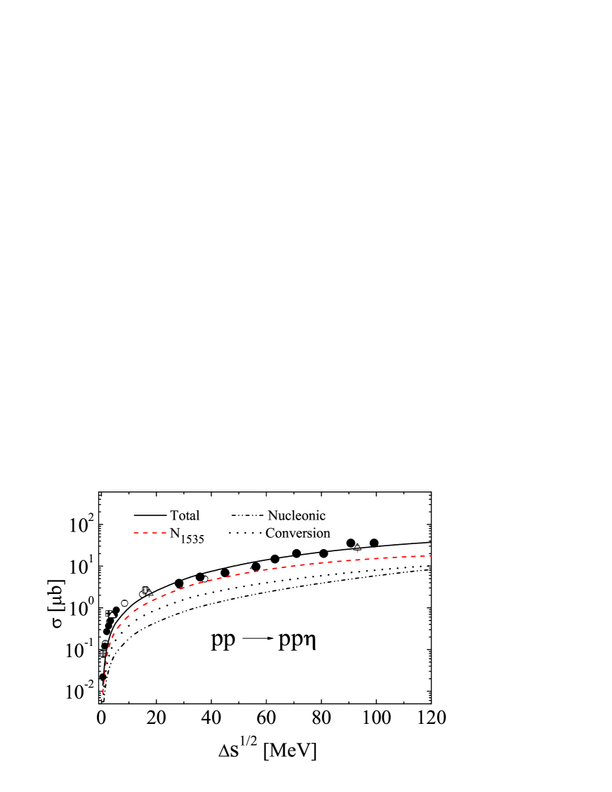
Figure 3: Total cross section for the reaction $pp\to pp\eta$ as a function of the excess energy $\Delta s^{1/2}=\sqrt{s}-2m-m_{\eta}$. The dot-dashed line corresponds to the nucleon current contribution (without resonances, Fig. 2a), while the dotted line is for the internal meson conversion diagram (Fig. 2b). The dashed curve exhibits the contribution of the $S_{11}(1535)$ resonance (nucleon resonance current in Fig. 2a). Contributions from $P_{11}(1440)$ and $D_{13}(1520)$ are smaller and not displayed. The solid curve is the total contribution with all interferences. Data are from Refs. etacalen ; etaexper ; etaangular ; etaexper1 ; etaexper2 ; etaexper3 ; error bars are suppressed.

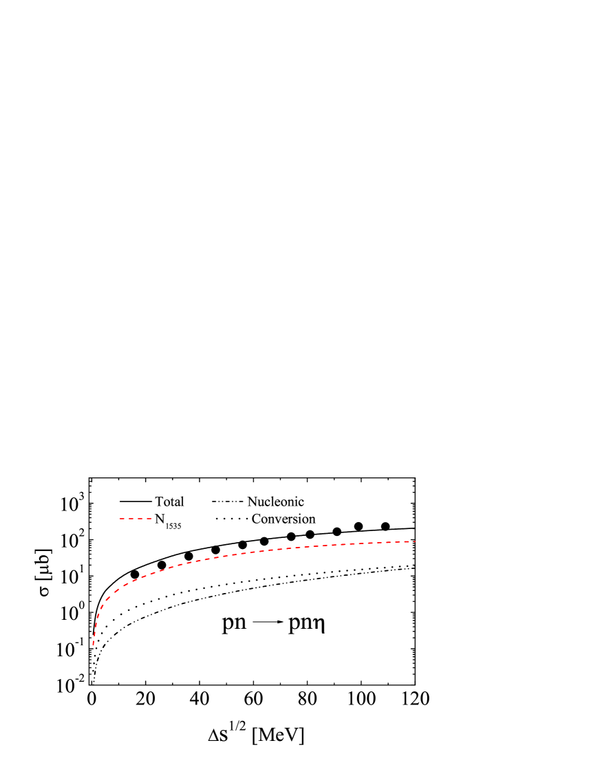
Figure 4: The same as in Fig. 3 but for the reaction $pn\to pn\eta$.

Results for the energy dependence of the total cross section $\sigma^{NN\to NN\eta}$, eq. (37), are presented in Figs. 3 and 4, for proton-proton and proton-neutron reactions, respectively. The amplitude $T_{NN\to NN\eta}^{(1)}$ represents a sum of nucleon, meson conversion and nucleon resonance currents, each of them being a sum over all the considered exchanged mesons (see Fig. 2). Using the parameters listed in Tabs. 1 and 2 the nucleon current contribution with parameters from the Bonn group bonncd is found to be fairly small in the present calculations (see dot-dashed curves).

Also the contribution from the conversion current (see doted curves) is not too large. The main contribution to the cross section comes from the nucleon resonance currents. Here it is worth mentioning that, in spite of the large number of the considered diagrams and the large number of the effective parameters, there is not too much freedom for fine-tuning of the cross section. As mentioned, most parameters are restricted by independent experiments and they cannot be varied in large intervals. We can slightly modify the less known parameters to achieve improvement of the overall description with data. In particular, in the present work we find a small contribution of the resonance $D_{13}(1520)$ at small energies, but a rather strong energy dependence due to $\pi$ and $\eta$ exchange diagrams with increasing energy. Therefore, in order to reduce the influence of the $D_{13}(1520)$ at large excess energies, for these diagrams the cut-off parameters have been chosen smaller than for others (see Tab. 2).

Note that, even achieving a good description of the cross section in proton-proton reactions, it is not a priory clear that the obtained set of parameters equally well describes also the proton-neutron reactions. The isospin dependence of the amplitude is determined by a subtle interplay of different diagrams with different exchange mesons (scalar, vector, isoscalar, isovector). Once the parameters for the $pp$ reaction are fixed, the $pn$ amplitude follows directly without further parameters (ISI and FSI are different for $pp$ and $pn$ systems, but fixed independently). Figure 4 demonstrates that the isospin dependence of the amplitude is correctly described with respect to available data.

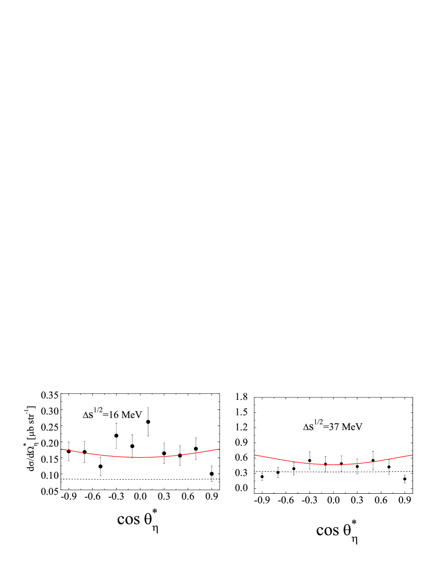
Figure 5: Angular distributions of $\eta$ mesons in the $pp$ center of mass system for the excess energies $\Delta s^{1/2}=16\,MeV$ (left panel) and $37\,MeV$ (right panel). The dotted lines depict the contribution of the conversion currents, while the solid lines correspond to the total differential cross section, including also nucleon and resonance currents and interferences. Data are from Ref. etaangular .

In Fig. 5 the angular distribution of $\eta$ mesons in the center of mass is presented for two excess energies, $\Delta s^{1/2}=16\,MeV$ (left panel) and $\Delta s^{1/2}=37\,MeV$ (right panel). Here a few comments are in order. Generally, at threshold-near energies the angular distributions are rather flat. That means that the total cross section at the corresponding energy is $\sigma^{tot}\propto 4\pi d\sigma/d\Omega^{*}$ and a quantitatively good description of the angular distribution $d\sigma/d\Omega^{*}$ provides, of course, also a good description of the total cross section. Therefore we compare our calculations with data at such an energy, where we achieve a better description of the total cross section (cf. Fig. 3). The other existing experimental data at similar energies (in particular, $\Delta s^{1/2}=15.5\,MeV$, etaangular ) differ from each other by an overall normalization factor, which can amount up to $40\%$ at these energies, see Ref. etacalen . Another important issue for the analysis of the angular distributions is the shape at forward and backward directions. The conversion current provides an upward ($\bigcup$) shape of the distributions, while the nucleon and nucleon-resonance currents generally give a downward ($\bigcap$) curve at forward and backward directions. Since in our calculations the contribution of the conversion current is much smaller than the one from the nucleon resonance current, the resulting angular distribution, albeit being rather flat, has however an upward ($\bigcup$) trend.

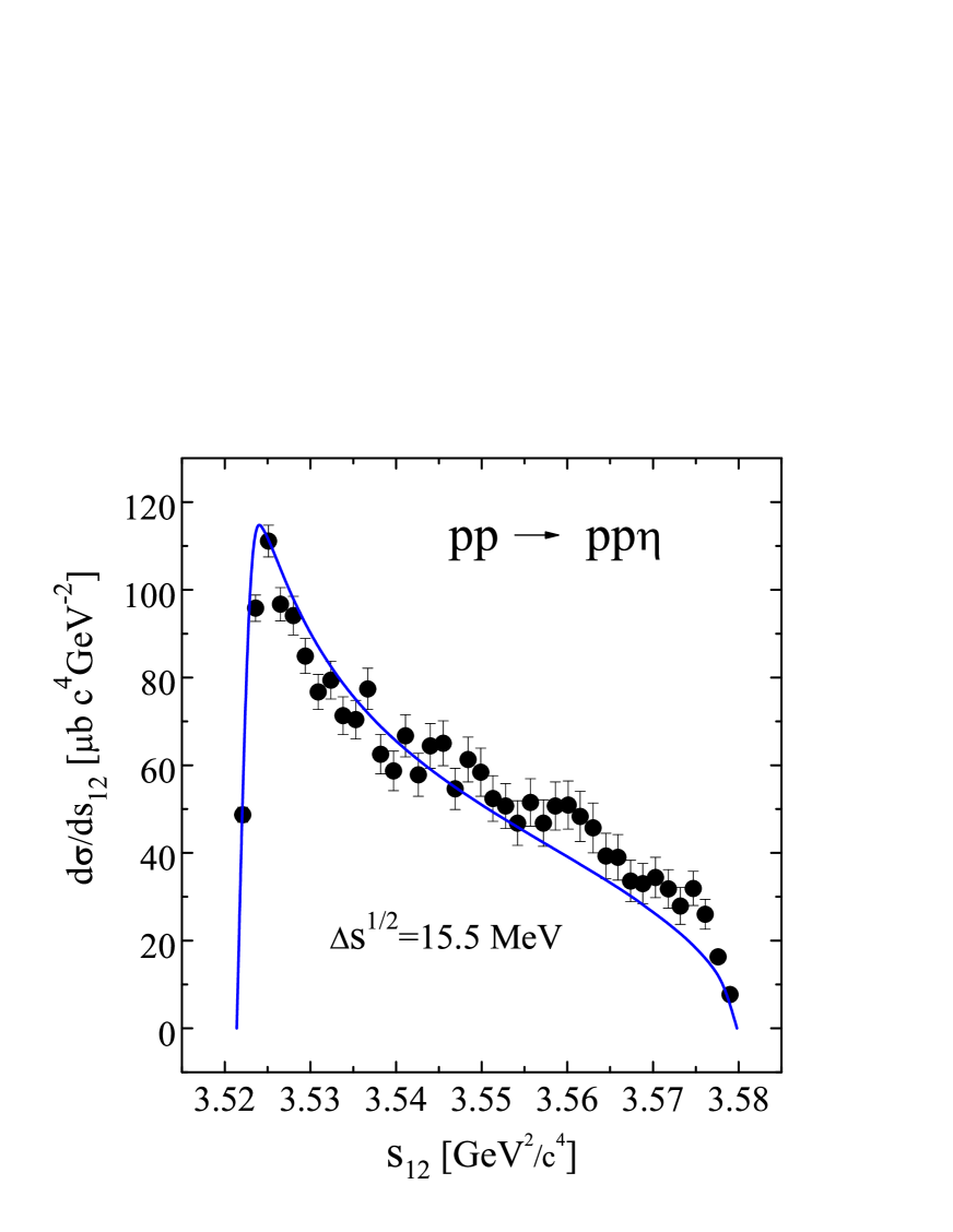
Figure 7: Distribution of the proton-proton invariant mass $s_{12}$ for the reaction $pp\to pp\eta$ at excess energy $\Delta s^{1/2}=15.5\,MeV$. Since there is an overall normalization uncertainty of data at $\Delta s^{1/2}=15.5-16.0\,MeV$ obtained by different groups our curve has been normalized to the data (see Ref. etacalen ; etaexper3 , normalization factor $\approx 1.4$). Data are from Ref. etaexper3 .

In Fig. 7 the invariant mass distribution of the two final protons is exhibited together with experimental data at an excess energy of $\Delta s^{1/2}=15.5\,MeV$. Since our total cross section has been optimized to describe the data at higher energies, $\Delta s^{1/2}>16\,MeV$, see Fig. 3, the calculated curve in Fig. 7 has been multiplied by a factor of $\approx 1.4$ obtained from an attempt to reconcile the data at $\Delta s^{1/2}=15.5\,MeV$ and $\Delta s^{1/2}=16\,MeV$ (relevant comments and discussion about the normalization of data can be found in Refs. etaangular ; etacalen ).

The mild discrepancy of the angular distribution in Fig. 5 and the slight underestimate of the total cross section data at $\Delta s^{1/2}\sim 10\,MeV$ let us argue that further reaction details could be accommodated. For instance, the $\bar{s}s$ shake-off considered in TitovBK may be included. This, however, deserves a separate consideration. As interim summary we believe to have at our disposal an appropriate description of the $\eta$ production cross section.

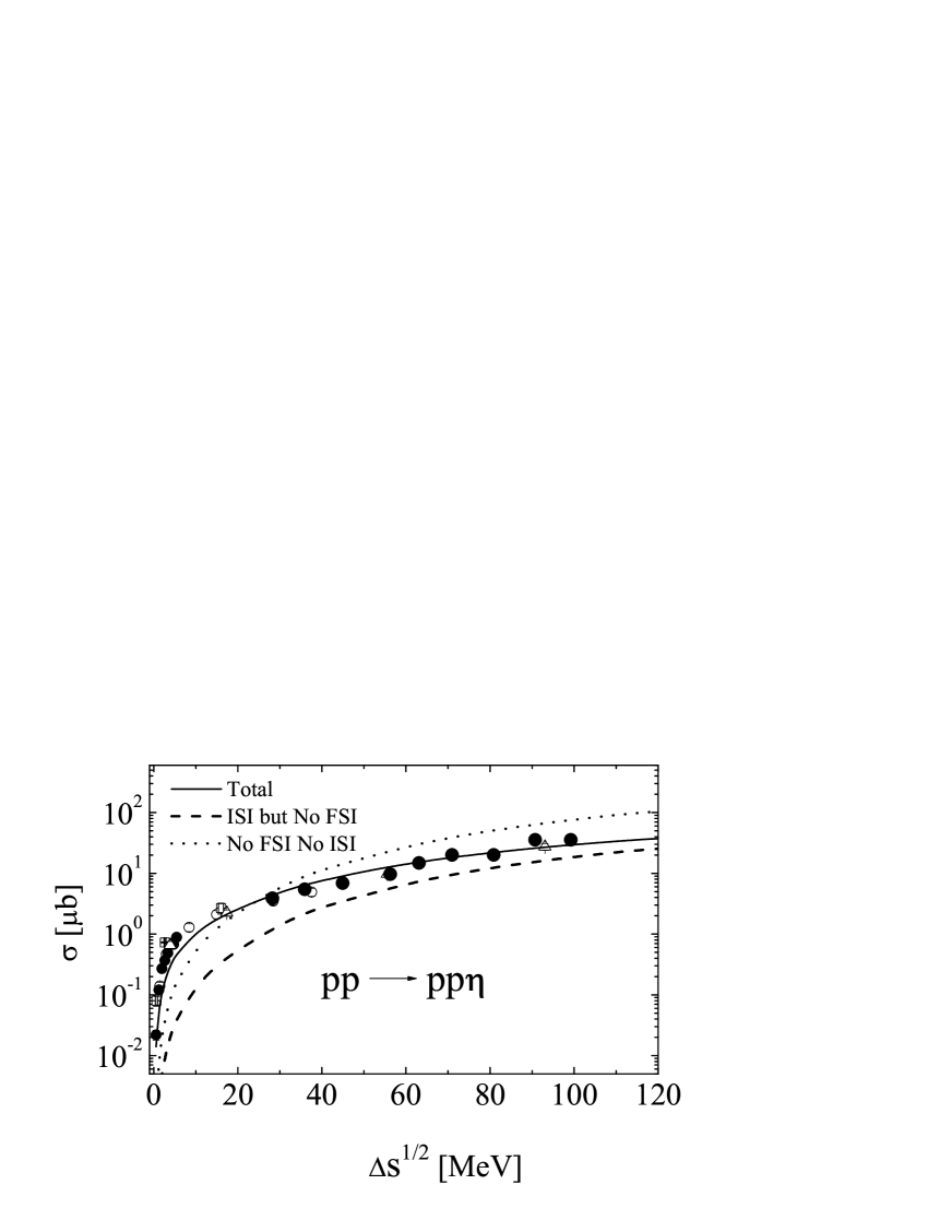
Figure 6: Effect of ISI and FSI for the reaction $pp\to pp\eta$. The dashed curve depicts the cross section when switching off the FSI, while the dotted curve is without both FSI and ISI. The solid curve and data are as in Fig. 3.

As mentioned in the introduction, in heavy-ion collisions a substantial part of di-electrons stem from Dalitz decays of $\eta$ mesons. In the same invariant mass region also $\Delta$ Dalitz and bremsstrahlung processes contribute to the total yield. It is, therefore, important to have some reliable cross sections for elementary $\eta$ production in $pp$ and $pn$ collisions as input for transport model simulations. Here one faces the problem whether the free cross sections (say, simply parameterizations of data) should be utilized or such ones where the FSI is ”switched off”, as in a dense hadronic environment the outgoing nucleons are not asymptotically free out-states. The same holds for the ISI. To have some indicator of the size of ISI and FSI effects we show in Fig. 6 the same as in Fig. 3 but with FSI switched off (dashed curve) or both ISI and FSI switched off (dotted curve, which may be called pure production cross section). A similar pattern holds for $pn\to pn\eta$ (not displayed). One observes indeed sizeable effects of ISI and FSI which point to the importance of a proper treatment of such effects in accurate many-body simulations.

V The Complete Reaction $\bf pp\to pp{\mbox{\boldmath$\eta$}}\to pp{\mathchar 28941\relax}e^{+}e^{-}$

In order to emphasize the dependence on the di-electron invariant mass we rewrite the integrated cross section (36) $d\sigma/ds_{\gamma^{*}}=\int ds_{\eta}\,(d\sigma/ds_{\eta}ds_{\gamma^{*}})$ in the form

$$\frac{d\sigma}{ds_{\gamma^{*}}}=\frac{2\alpha}{3\pi^{2}}|F_{\eta\gamma\gamma^{*}}(s_{\gamma^{*}})|^{2}\frac{Br(\eta\to 2\gamma)}{m_{\eta}^{2}}{\cal I}(s_{\gamma^{*}}),$$ (40)

$${\cal I}(s_{\gamma^{*}})\equiv\int\limits_{1}^{\xi_{max}}d\xi\frac{(\xi-1)^{3}}{\xi\,a}\frac{b}{(\xi-a)^{2}+b^{2}}\sigma^{tot}_{NN\to NN\eta}(\xi),$$ (41)

where we introduced dimensionless variables $a$, $b$ and $\xi$

$$a\equiv\frac{m_{\eta}^{2}}{s_{\gamma^{*}}};\qquad b\equiv\frac{m_{\eta}\,\Gamma_{\eta}}{s_{\gamma^{*}}},\qquad\xi\equiv\frac{s_{\eta}}{s_{\gamma^{*}}},\quad\xi_{max}=\frac{(\sqrt{s}-2m_{\eta})^{2}}{s_{\gamma^{*}}}.$$ (42)

$d\sigma/ds_{\gamma^{*}}$ may be considered as normalized contribution to the di-electron invariant mass spectrum mediated by the $\eta$ Dalitz decay.

Since the total width of the $\eta$ meson is fairly small, the parameter $b$ in (41) provides a very sharp maximum of the integrand function at $\xi=a$ as long as the parameter obeys $a>1$ (or, equivalently, the di-electron invariant mass fulfills $s_{\gamma}^{*}<m_{\eta}^{2}$). This allows to pull out the smooth function $\sigma^{tot}_{NN\to NN\eta}(\xi=a)$ from the integral and to calculate it at $s_{\eta}=m_{\eta}^{2}$, i.e. for the on-shell $\eta$ meson. The remaining part can be calculated analytically. However, for $a<1$, when the di-electron mass is larger than the $\eta$ pole mass, the integrand does not exhibit anymore a resonant shape and the integral ought to be calculated numerically.

Equation (40) shows that the di-electron invariant mass distribution $d\sigma/ds_{\gamma^{*}}$ is proportional to the transition form factor $F_{\eta\gamma\gamma^{*}}(s_{\gamma^{*}})$ so that measurements of this distribution provide direct experimental information about the FF. It can be checked that up to $a\sim 1.035$ (corresponding to $s_{\gamma^{*}}\simeq 0.29\,GeV^{2}$) the smooth part of the integrand, $\displaystyle\frac{b(\xi-1)^{3}}{a\xi}\,\sigma^{NN\to NN\eta}(\xi)$, can be pulled out from the integral at $\xi=a$ obtaining

$${\cal I}(s_{\gamma^{*}})=\displaystyle\frac{\pi(a-1)^{3}}{a^{2}}\,\sigma^{NN\to NN\eta}(s_{\eta}=m_{\eta}^{2}).$$ (43)

Equations (40 - 43) allow then to define an experimentally measurable ratio which is directly proportional to the form factor squared

$$R(s_{\gamma^{*}})=\frac{d\sigma/ds_{\gamma^{*}}}{\left.\left(d\sigma/ds_{\gamma^{*}}\right)\right|_{s_{\gamma^{*}}=s_{\gamma^{*},min}}}\frac{s_{\gamma^{*}}}{s_{\gamma^{*},min}}\left(\frac{1-s_{\gamma^{*},min}/m_{\eta}^{2}}{1-s_{\gamma^{*}}/m_{\eta}^{2}}\right)^{3}=\frac{|F_{\eta\gamma\gamma^{*}}(s_{\gamma^{*}})|^{2}}{|F_{\eta\gamma\gamma^{*}}(s_{\gamma^{*},min})|^{2}}$$ (44)

where $s_{\gamma^{*},min}$ is the minimum value accessible experimentally (in the ideal case this is the kinematical limit $s_{\gamma^{*},min}=4\mu_{e}^{2}$ with electron mass $\mu_{e}$). At low enough values of $s_{\gamma^{*},min}$, the transition FF is close to its normalization point $F_{\eta\gamma\gamma^{*}}(0)=1$ and the ratio (44) is just the transition FF as a function of $s_{\gamma^{*}}$.

As $a$ approaches unity keeping the maximum position still within the integration range, one can again withdraw from the integral the smooth function $\sigma^{NN\to NN\eta}$ at $s_{\eta}=m_{\eta}^{2}$. However, now the function $(\xi-1)^{3}/\xi$ can not be considered as smooth enough and must be kept under the integration. Nevertheless, even in this case the remaining integral can be computed analytically (see Appendix B) and one can still define a ratio analogous to (44) which allows for an experimental investigation of the FF near the free $\eta$ threshold ($s_{\gamma^{*}}\to m_{\eta}^{2}$). At $s_{\gamma^{*}}>m_{\eta}^{2}$ the integral ${\cal I}(s_{\gamma^{*}})$ does not have anymore a sharp maximum and it must be calculated numerically as mentioned above.

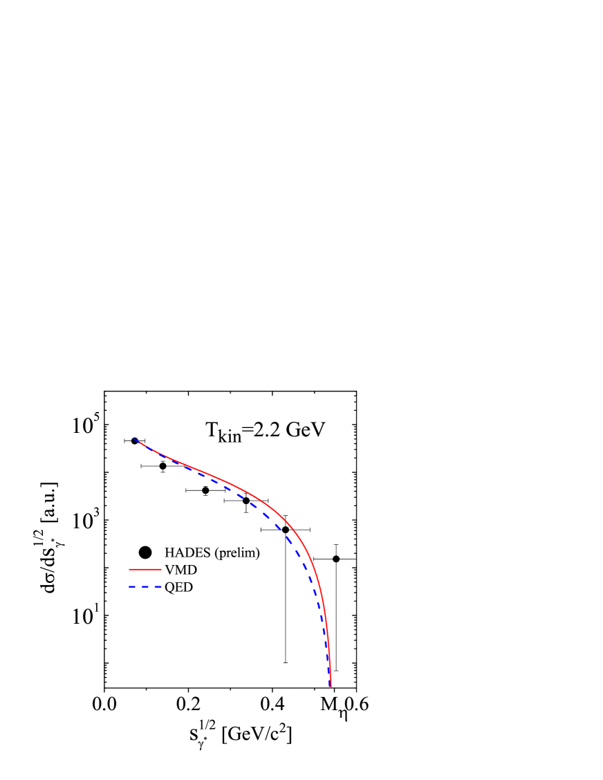
Figure 8: Invariant mass distribution of di-electrons produced by Dalitz decay of $\eta$ mesons in the reaction $pp\to pp\gamma e^{+}e^{-}$ at initial kinetic energy $T_{kin}=2.2\,GeV$. The solid line is for results with the $\eta\gamma\gamma^{*}$ transition FF computed within the VMD model, while the dashed line corresponds to a pure QED calculation of the $\eta\gamma\gamma^{*}$ vertex, i.e., for $|F_{\eta\gamma\gamma^{*}}|^{2}=1$. The position of $\eta$ pole mass is exposed. Preliminary experimental data are from Ref. hadeseta .

In Fig. 8 the di-electron invariant mass distribution $d\sigma/ds_{\gamma^{*}}^{1/2}$ is exhibited as a function of the invariant mass $s_{\gamma^{*}}^{1/2}$ calculated from formula (40). The solid curve employs the transition FF $F_{\eta\gamma\gamma^{*}}(s_{\gamma^{*}})$ calculated within the VMD model LandPhysRep

$$F_{\eta\gamma\gamma^{*}}^{VMD}(s_{\gamma^{*}})=\displaystyle\frac{m_{\rho}^{2}}{s_{\gamma^{*}}-(m_{\rho}-\frac{i}{2}\Gamma_{\rho})^{2}}$$ (45)

with standard values for $m_{\rho}$ and $\Gamma_{\rho}$ dataGroup . (Note that in the kinematical region of interest the $\rho$ contribution is sufficient.) The dashed curve in Fig. 8 is for the pure QED part, i.e. without accounting for the strong form factor, i.e. with $F_{\eta\gamma\gamma^{*}}(s_{\gamma^{*}})=1$. The experimental data in Fig. 8 are preliminary results from HADES hadeseta . It is clearly seen that without FF the calculated cross section rapidly drops as $s_{\gamma^{*}}^{1/2}\to m_{\eta}$, while inclusion of the FF only mildly modifies the shape (factor 2 increase at $m_{\gamma^{*}}\sim 400\,MeV$ High precision data are needed to arrive at a firm conclusion on the validity of the employed VMD FF.

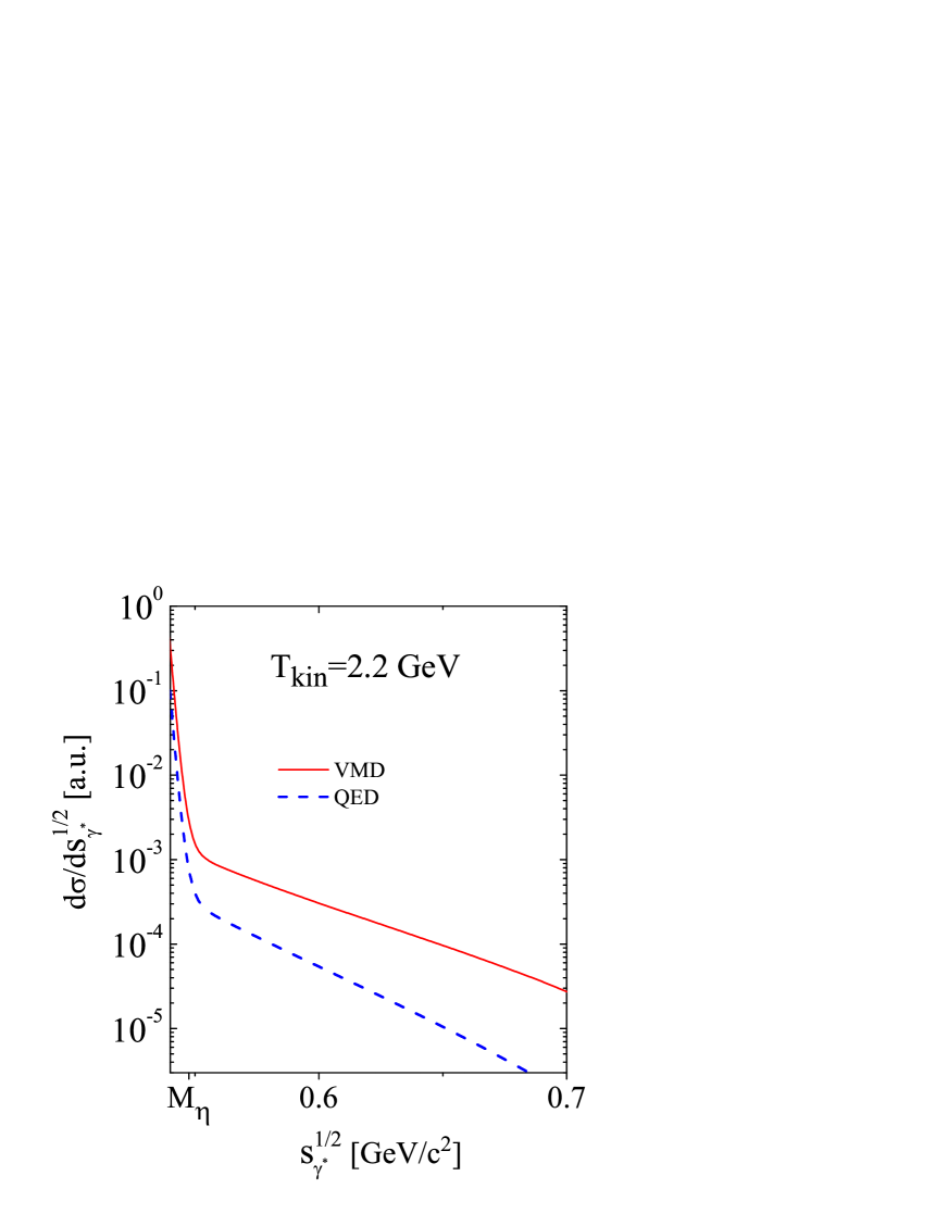
Figure 9: The same as in Fig. 8 but in the kinematical region beyond the ”$\eta$ threshold”, i.e. for di-electron masses larger than the $\eta$ pole mass being accessible for intermediate off-shell $\eta$ mesons.

With increasing $s_{\gamma^{*}}^{1/2}$, the effect of the FF becomes more and more pronounced. This can be visualized if one calculates the $e^{+}e^{-}$ mass distribution beyond the free $\eta$ meson pole mass, i.e. at $s_{\gamma^{*}}^{1/2}>m_{\eta}$. Figure 9 exhibits the behavior of the mass distribution at large values of $s_{\gamma^{*}}^{1/2}$. The effect of the FF increases noticeably at large values of $s_{\gamma^{*}}$. This is of interest since, as mentioned, the VMD calculations provides a good description of the on-shell $\eta$ meson FF in the range $s_{\gamma^{*}}<m_{\eta}^{2}$. An investigation of the FF at $s_{\gamma^{*}}>m_{\eta}^{2}$ can provide information of the relevance of the VMD model for off-shell hadrons at kinematical limit. In particular, when calculating Dalitz type processes with (off-shell) vector mesons created via bremsstrahlung off nucleon resonances, one usually estimates the couplings in the corresponding vertices from the radiative decay off an on-shell resonance with applying the VMD model. An additional justification of such a procedure can be obtained from investigating the transition FF beyond the on-mass shell limit. It should be noted, however, that severe background processes will make difficult an identification of the $\eta$ Dalitz yield in this kinematical region.

VI Summary

In summary we have analyzed the di-electron production from Dalitz decays of $\eta$ mesons produced in $pp$ collisions at intermediate energies. The corresponding cross section has been calculated within an effective meson-nucleon approach with parameters adjusted to a large extent to describe the free vector meson production in $NN$ reactions near the threshold. We argue that by studying the invariant mass distribution of the final $e^{+}e^{-}$ system in a large kinematical interval of di-electron masses, one can directly measure the $\eta$ meson transition form factor $F_{\eta\gamma\gamma^{*}}$ in, e.g., $pp$ collisions. Such experiments are already performed and will be further improved at HADES. Our results may serve as prediction for these forthcoming experiments. The uncertainties of such a procedure depend upon the scale of the background processes and is expected to be small if the interference is destructive ourFF . Experimental information on transition form factors is useful for testing QCD predictions of hadronic quantities in the non-perturbative domain.

Appendix A Coupling constants for spin-$\frac{3}{2}$ resonances

The coupling constants of the spin-$\frac{3}{2}$ resonance $D_{13}(1520)$ can be estimated from the known decay widths. For instance, for the decay $D_{13}(1520)\to N\eta$ one has

$$\Gamma_{N^{*}\to N\eta} = \frac{1}{8\pi}\frac{\sqrt{[m_{N^{*}}^{2}-(m_{N}-m_{\eta})^{2}][m_{N^{*}}^{2}-(m_{N}+m_{\eta})^{2}]}}{2m_{N^{*}}^{3}}\frac{g^{2}_{\eta NN^{*}}}{m_{\eta}^{2}}\frac{1}{4}\sum_{spins}|{\cal M}|^{2}$$ (46)

$$= \frac{1}{64\pi m_{N^{*}}^{3}}\sqrt{[m_{N^{*}}^{2}-(m_{N}-m_{\eta})^{2}][m_{N^{*}}^{2}-(m_{N}+m_{\eta})^{2}]}\frac{g^{2}_{\eta NN^{*}}}{m_{\eta}^{2}}\frac{2}{3}\left(\frac{(P_{N^{*}}q_{\eta})}{m_{N^{*}}^{2}}-m_{\eta}^{2}\right)$$

$$\times {\rm Tr}\left[(\hat{P}_{N}+m_{N})\gamma_{5}(\hat{P}_{N^{*}}+m_{N^{*}})\gamma_{5})\right],$$

where for the spin-$\frac{3}{2}$ particles we use the Rarita-Schwinger spinors ${\cal U}^{\mu}(P_{N^{*}},\bar{s})$ for the spin $\bar{s}$ summation with the relation

$$\sum_{\bar{s}}{\cal U}^{\mu}(P_{N^{*}},\bar{s})\bar{\cal U}^{\nu}(P_{N^{*}},\bar{s}) = (\hat{P}_{N^{*}}+m_{N^{*}})$$ (47)

$$\times \left(-g_{\mu\nu}+\frac{\gamma^{\mu}\gamma^{\nu}}{3}+\frac{(\gamma^{\mu}P_{N^{*}}^{\nu}-\gamma^{\nu}P_{N^{*}}^{\mu})}{3m_{N^{*}}}+\frac{2P_{N^{*}}^{\mu}P_{N^{*}}^{\nu}}{3m_{N^{*}}^{2}}\right).$$

We use the short hand notation $\hat{p}=(p\cdot\gamma)$. Equation (46) provides slightly larger coupling constants than that used in Ref. nakayamaEta in which, besides the decay widths, the coupling constants have been adjusted to fit also other processes involving $D_{13}(1520)$. An analog equation hold for $D_{13}(1520)\to N\pi$. In the present paper we take $g_{\pi NN^{*}}=1.55$ and $g_{\eta NN^{*}}=8.3$, see Tab. 2.

Appendix B Integration over the variable $\bf s_{\mbox{\boldmath$\eta$}}$

Since the parameter $b$ in eq. (41) is very small in the whole kinematical region of $s_{\gamma^{*}}$ the integrand has a sharp maximum around $\xi=a$. If $a>x_{min}=1$ then the maximum is located inside the integration interval of $\xi$ and one can take advantage of the smoothness of the $\eta$ production cross section $\sigma^{NN\to NN\eta}$ to withdraw it from the integral. Then

$${\cal I}_{1}(\xi) \equiv \int d\xi\frac{(\xi-a)^{3}}{\xi}\frac{b/a}{(\xi-a)^{2}+b^{2}}$$ (48)

$$= \frac{b}{a}\xi+\frac{b}{a(a^{2}+b^{2})}\left[-\ln\xi+\frac{1}{2}\ln\left((\xi-a)^{2}+b^{2}\right)\left(2a^{3}-3a^{2}+2ab^{2}-3b^{2}+1\right)\right.$$

$$+ \left.\frac{1}{b}{\rm arctan}\left(\frac{\xi-a}{b}\right)\left(a^{4}-3a^{3}+3a^{2}-a-3ab^{2}-b^{4}+3b^{2}\right)\right].$$

It is seen that in case when $a\gg 1$, $b\ll 1$ the term $b\xi/a$ and terms containing logarithms in (48) can be disregarded:

$${\cal I}_{1}(\xi) \simeq \frac{(a-1)^{3}}{a^{2}}{\rm arctan}\left(\frac{\xi-a}{b}\right),$$ (49)

$${\cal I}_{1}(\xi_{max})-{\cal I}_{1}(\xi_{min}) \simeq \pi\frac{(a-1)^{3}}{a^{2}}.$$ (50)

This corresponds to the case when in eq. (41) one withdraws from the integral both the production cross section $\sigma^{NN\to NN\eta}$ and the combination $(\xi-1)^{3}/\xi$ at $\xi=a$. Note that eq. (48) is a good approximation even for $a<1$, if $a+b>1$, i.e. for $a$ in the $b$ vicinity of unity.

Figure 2: Diagrams for the process $NN\to NN\gamma e^{+}e^{-}$ within an effective meson-nucleon theory. a) Dalitz decays of $\eta$ mesons from bremsstrahlung like diagrams. The intermediate baryon $N^{*}$ (triple line) can be either a nucleon or one of the nucleon resonances $S_{11}(1535)$, $P_{11}(1440)$ or $D_{13}(1520)$. Analog diagrams for the emission from Fermion line $N_{2}$. b) Dalitz decay of $\eta$ mesons from internal meson conversion. Exchange diagrams for identical nucleons in exit channel are not displayed.

References

- (1) H. Agakishev et al. (HADES collaboration), Phys. Rev. Lett. 98 (2007) 052302
- (2) H.W. Barz, B. Kämpfer, Gy. Wolf, M. Zetenyi, nucl-th/0605036.
- (3) L.P. Kaptari, B. Kämpfer, Nucl. Phys. A764 (2006) 338.
-
(4)
P. Salabura et al. (HADES Collaboration), Acta Phys. Pol. B35 (2004) 1119;
R. Holzmann et al. (HADES Collaboration), Prog. Part. Nucl. Phys. 53 (2004) 49. - (5) L.G. Landsberg, Phys. Rep. 128 (1985) 301.
- (6) I. Fröhlich et al. (HADES collaboration), nucl-ex/0610048.
-
(7)
G. Fäldt, C. Wilkin, Phys. Scripta 64 (2001) 427;
U. Tengblad, G. Fäldt, C. Wilkin, Eur. Phys. J. A25 (2005) 267;
C. Wilkin, U. Tengblad, G. Fäldt, Acta Phys. Slov. 56 (2005) 205. - (8) A.B. Santra, B.K. Jain, Nucl. Phys. A634 (1998) 309.
- (9) E. Gedalin, A. Moalem, L. Razodolskaja, Nucl. Phys. A634 (1998) 368.
-
(10)
K. Nakayama, J. Speth, T.-S. Lee, Phys. Rev. C65 (2002) 045210;
K. Nakayama, H.F. Arellano, J.W. Durso, J. Speth, Phys. Rev. C61 (1999) 024001;
K. Nakayama, J. Haidenbauer, C. Hanhart, J. Speth, Phys. Rev. C68 (2003) 045201. - (11) V. Shklyar, H. Lenske. U. Mosel, nucl-th/0611036.
- (12) L.P. Kaptari, B. Kämpfer, Eur. Phys. J. A23 (2005) 291.
-
(13)
L.P. Kaptari, B. Kämpfer, Eur. Phys. J. A14 (2002) 211;
L.P. Kaptari, B. Kämpfer, J. Phys. G30 (2004) 1115. -
(14)
U.-G. Meißner, Phys. Rep. 161 (1988) 213;
N.M. Kroll, T.D. Lee, B. Zumino, Phys. Rev. 157 (1967) 1376. - (15) H.B. O’Connell, B.C. Pearce, A.W. Thomas, A.G. Williams, Prog. Part. Nucl. Phys. 39 (1997) 201.
-
(16)
A.V. Anisovich, V.V. Anisovich, V.A. Nikonov, Eur. Phys. J. A12 (2001) 103;
A.V. Anisovich, V.V. Anisovich, V.A. Nikonov, hep-ph/0305216. -
(17)
A. Faessler, C. Fuchs, M. Krivoruchenko, Phys. Rev. C61 (2000) 035206;
H.C. Dönges, M. Schäfer, U. Mosel, Phys. Rev. C51 (1995) 950. - (18) L.P. Kaptari, B. Kämpfer, nucl-th/0610068, Eur. Phys. J. A31 (2007) in print.
- (19) S. Eidelman et al. (Particle Data Group), Phys. Lett. B592 (2004) 1.
- (20) R.I. Dzhelyadin, S.V. Golovkin, M.V. Gritsuk, D.B. Kakauridze et al., Phys. Lett. B84 (1979) 143; Phys. Lett. B88 (1979) 379.
- (21) R.I. Dzhelyadin, S.V. Golovkin, A.S. Konstantinov, V.P. Kubarovski et al., Phys. Lett. B102 (1981) 296.
- (22) V.A. Viktorov, S.V. Golovkin, R.I. Dzhelyadin, V.P. Kubarovski et al., Yad. Fiz. 32 (1980) 998, 1002, 1005; Phys. Lett. B94 (1980) 548.
- (23) M.F.M. Lutz, B. Friman, M. Soyeur, Nucl. Phys. A713 (2003) 97.
- (24) B. Friman, M. Soyeur, Nucl. Phys. A600 (1996) 477.
- (25) E. Byckling, K. Kajantie, ”Particle Kinematics”, John Wiley & Sons 1973.
- (26) J.W. Durso, Phys. Lett. B184 (1987) 348.
- (27) M. Benmerrouche, N.C. Mukhopadhyay, Phys. Rev. D51 (1995) 3237.
- (28) R.M. Davidson, N.C. Mukhopadhyay, R.S. Wittman, Phys. Rev. D43 (1991) 71.
- (29) M.J. Dekker, P.J. Brussaard, J.A. Tjon, Phys. Rev. C49 (1994) 2650.
- (30) A.I. Titov, B. Kämpfer, B.L. Reznik, Phys. Rev. C65 (2002) 065202.
- (31) M.Post, S. Leupold, U. Mosel, Nucl. Phys. A689 (2001) 753.
- (32) H.T. Williams, Phys. Rev. C39 (1989) 02339.
- (33) R.E. Behrends, C. Fronsdal, Phys. Rev. 106 (1957) 345.
- (34) R. Machleidt, Adv. Nucl. Phys. 19 (1989) 189;
- (35) C. Hanhart, K. Nakayama, Phys. Lett. B454 (1999) 176.
- (36) http://said-hh.edsy.de
- (37) J. Gillespie, ” Final State Interactions”, Holden-Day Advanced Physics Monographs, 1964.
- (38) A.I. Titov, B. Kämpfer, B.L. Reznik, Eur. Phys. J. A7 (2000) 543.
- (39) H. Calen, J. Dyring, G. Fäldt, K. Fransson et al., Phys. Lett. B458 (1999) 190.
-
(40)
H. Calen, S. Carius, K. Fransson, L. Gustafsson et al., Phys. Lett. B366 (1996) 39;
H. Calen, J. Dyring, K. Fransson, L. Gustafsson et al., Phys. Rev. Lett. 79 (1997) 2642;
H. Calen, J. Dyring, K. Fransson, L. Gustafsson et al., Phys. Rev. C58 (1998) 2667. - (41) A.I. Titov, B. Kämpfer, V.V. Shklyar, Phys. Rev. C 59 (1999) 999.
-
(42)
E. Chiavassa, G. Dellacasa, N. De Marco, C. De Oliveira Martins et al.,
Phys. Lett. B322 (1994) 270;
F. Hibou, O. Bing, M. Boivin, P. Courtat et al., Phys. Lett. B438 (1998) 41;
J. Smyrski, P. Wüstner, J.T. Balewski, A. Budzanowski et al., Phys. Lett. B474 (2000) 182. -
(43)
F. Balestra, Y. Bedfer, R. Bertini, L.C. Bland et al., Phys. Lett. B491 (2000) 29;
F. Balestra, Y. Bedfer, R. Bertini, L.C. Bland et al., Phys. Rev. C69 (2004) 064003. - (44) A.M. Bergodolt, G. Bergodolt, O. Bing, A. Bouchakour et al., Phys. Rev. D48 (1993) R2969.
-
(45)
P. Moskal, H.-H. Adam, A. Budzanowski, R. Czyzkiewich et al.,
Phys. Rev. C69 (2004) 025203;
see also EPAPS Document No. E-PRVCAN-68-015312
(http://www.aip.org/pubservs/epaps/html).