Neutron-³H potentials and the ⁵H-properties

Abstract

The continuum resonance spectrum of ⁵H (³H+$n$+$n$) is investigated by use of the complex scaled hyperspherical adiabatic expansion method. The crucial ³H-neutron potential is obtained by switching off the Coulomb part from successful fits to ³He-proton experimental data. These two-body potentials must be expressed exclusively by operators conserving the nucleon-core mean field angular momentum quantum numbers. The energies $E_{R}$ and widths $\Gamma_{R}$ of the $1/2^{+}$ ground-state resonance and the lowest two excited $5/2^{+}$ and $3/2^{+}$-resonances are found to be $(1.6,1.5)$ MeV, $(2.8,2.5)$ MeV and $(3.2,3.9)$ MeV, respectively. These results agree with most of the experimental data. The energy distributions of the fragments after decay of the resonances are predicted.

PACS:  21.45.+v, 31.15.Ja, 25.70.Ef

1 Introduction

Recent advances in experimental techniques have opened the door to investigate superheavy hydrogen isotopes, ⁵H and ⁷H. None of them, nor ⁴H, have bound states, while ³H is well bound with the neutron separation energy of 6.26 MeV. At the neutron dripline, where one neutron becomes unbound, the structure has been successfully described as an ordinary nuclear core surrounded by weakly bound or unbound neutrons [1]. It is therefore natural to describe the ^AH nuclei ($A>3$) as a bound triton-core, denoted $t$ or ³H, surrounded by $A-3$ neutrons.

In the present work we focus on ⁵H ($t$+$n$+$n$), for which the experimental data are controversial. A summary of the different experimental data and techniques can be found in [2]. In [3] the ⁵H ground state is found to be a 1/2⁺ state with energy $E_{R}=1.7\pm 0.3$ MeV and width $\Gamma_{R}=1.9\pm 0.4$ MeV. Similar results were found in [4], where the authors quote an energy of 1.8 MeV and a width of 1.3 MeV, and in [5], where the 1/2⁺ ground state of ⁵H is located at 2 MeV with a width of 2.5 MeV. In [6, 7] a broad structure is observed in the ⁵H energy distribution after proton knockout from ⁶He, that was interpreted as a $1/2^{+}$ resonance at around 3 MeV. No evidence for a narrow resonance in the $t+n+n$ system was obtained in contrast to [8], where two rather narrow resonances were reported at $1.8\pm 0.1$ MeV and $2.7\pm 0.1$ MeV with widths less than $0.5$ MeV. In [9] even a higher energy of $5.5\pm 0.2$ MeV and a larger width of $5.4\pm 0.6$ MeV are given for the ⁵H ground state, which is consistent with the results presented in [10].

The data obtained for the excited 3/2⁺ and 5/2⁺ states tend to agree that these resonances are broad structures, almost degenerate, with energies varying between 2.5 MeV [4, 5] and more than 10 MeV [9]. Different theoretical calculations concerning ⁵H are available [11, 12, 13, 14, 15]. In general they agree in placing the 1/2⁺ ground state between 2 and 3 MeV except [11] where 6 MeV is reported. The widths of these resonances are only rough estimates except for the more complete computation in [15].

The first three-body calculation of ⁵H [12] used the hyperspheric harmonic expansion method with a neutron-triton interaction obtained from fits to the scarce amount of experimental phase shifts [16]. The interaction is not consistent with the available ³He-proton phase shifts. The resonances are obtained from an analysis of the three-body phase shifts and the bumps observed in the computed missing mass spectra. The authors find a ground state energy at around 2.5-3.0 MeV. However extraction of the resonance properties from the missing mass spectra is not unambiguous, since it requires a full description of the process used to populate the ⁵H-states (initial state, reaction mechanism, final state interactions). This problem is discussed in detail in [17], which shows how different descriptions of the reaction process can provide different properties of the ⁵H ground state.

The origin of these uncertainties is often related to a mismatch between experimental and theoretical definitions of resonances. The experimental analyses of resonance energies and widths are most often consistent with the definition of resonances as generalized eigenstates of a given system, i.e. when they are defined as poles of the $S$-matrix in the fourth quadrant of the complex energy plane. With this assumption the reaction mechanism used to populate the resonances becomes unimportant. The only essential ingredients in the calculation of three-body resonances are then the different two-body interactions.

The main theoretical problem is that the resonance wave functions diverge asymptotically, which makes them difficult to disentangle from ordinary non-resonant continuum wave functions. Different methods are available to overcome this problem. For instance, the analytic continuation of the coupling constant [18] is used in [13] to investigate ⁵H, and the ground state is found at around 3 MeV with a width varying between 1 and 4 MeV.

An efficient method to obtain the $S$-matrix poles is the complex scaling method [19, 20], where all spatial coordinates are rotated into the complex plane by a judicially chosen angle $\theta$. In this way, provided that $\theta$ is larger than the argument of the resonance, the wave function of the resonance falls off exponentially exactly as for a bound state. In [15] the complex scaling method together with the microscopic three-cluster model is used to investigate the ⁵H nucleus. An effective nucleon-nucleon interaction is used to construct the neutron-triton potential. The energy and width of the 1/2⁺ ground state are then found to be 1.59 MeV and 2.48 MeV, respectively, while the excited 3/2⁺ and 5/2⁺ states are found almost degenerate at 3.0 MeV, and with widths above 4 MeV.

In the last years it has been shown that the hyperspherical adiabatic expansion method [21] is an efficient tool to obtain three-body bound states and resonances when combined with the complex scaling method. The method has been applied successfully to investigate systems like ⁶He, ⁶Be, ⁶Li, ¹¹Li, ¹²C, and ¹⁷Ne, [22, 23, 24, 25], where the agreement with the available experimental data is found to be remarkably good. We therefore believe that a similar investigation of the properties of ⁵H can help to clarify the existing uncertainties.

The paper is organized as follows: In section 2 we introduce the method and discuss in detail the two-body neutron-triton interaction, that is the most crucial ingredient in the calculation. In section 3 the properties of ⁴H are discussed. The three-body results are shown in section 4. The energy distributions of the particles after decay of the three-body resonances are given in section 5. We then finish in section 6 with the summary and the conclusions.

2 Crucial ingredients

The adiabatic expansion method with hyperspherical coordinates and the Faddeev decomposition is described for three-body systems in [21]. The extension to compute resonances with complex rotation for these systems is described in [23]. We shall here specify the details necessary to understand the subsequent discussion. First we sketch the method and then we discuss in detail the decisive neutron-triton interaction.

2.1 Notation and parameters

We define the hyperradius $\rho$ by

$$m(m_{1}+m_{2}+m_{3})\rho^{2}=\sum^{3}_{i<j}m_{i}m_{j}\left(\mbox{\boldmath$r$}_{i}-\mbox{\boldmath$r$}_{j}\right)^{2}\;,$$ (1)

where $m_{i}$ and $\mbox{\boldmath$r$}_{i}$ are the mass and coordinate of particle number $i$. The mass $m$ is arbitrary and here chosen as the nucleon mass. All other relative coordinates are dimensionless angles collectively denoted by $\Omega$. The hyperradius is rotated by an angle $\theta$ into the complex plane by multiplication with $\exp(i\theta)$.

The total wave function $\Psi^{(JM)}$ with total angular momentum, $J$, and projection, $M$, is expanded on the complete set $\Phi^{(JM)}_{n}$ of adiabatic angular wave functions obtained for a fixed value $\rho$ [21], i.e.

$$\Psi^{(JM)}=\frac{1}{\rho^{5/2}}\sum_{n}f_{n}(\rho)\Phi_{n}^{(JM)}(\rho,\Omega)$$ (2)

$$\Phi_{n}^{(JM)}(\rho,\Omega)=\sum_{i=1}^{3}\phi_{n}^{(i)}(\rho,\Omega_{i})$$ (3)

where $\phi_{n}^{(i)}$ is the Faddeev component related to the Jacobi system labeled by $i$. The expansion coefficients are the radial wave functions, $f_{n}(\rho)$, obeying a coupled set of radial equations obtained by projecting the complex scaled Faddeev equations on the adiabatic angular wave functions. They are exponentially decaying for resonances when the rotation angle $\theta$ of the hyperradius is larger than that corresponding to the three-body resonance. Then both real and imaginary parts of the resonance energy, $E_{0}=E_{R}-iE_{I}$, , are determined by the boundary condition of $f_{n}$, i.e.

$$f_{n}(\kappa\rho e^{i\theta})\rightarrow\sqrt{\rho}H_{K+2}^{(1)}(|\kappa|\rho e^{i(\theta-\theta_{R})})$$ (4)

$$\rightarrow\exp\Big{(}{-|\kappa|\rho\sin{(\theta-\theta_{R})}}+i\left(|\kappa|\rho\cos{(\theta-\theta_{R})}-K\pi/2+3\pi/4\right)\Big{)},$$

where $\theta_{R}$ is the argument of the complex momentum, $\kappa=\sqrt{2mE_{0}/\hbar^{2}}=|\kappa|\exp(-i\theta_{R})$, and $H_{K+2}^{(1)}$ is the Hankel function of the first kind.

The two-body interaction is the all-decisive input. In general, the low-energy scattering properties of all pairs of particles should be reproduced. A smaller amount of data like scattering length and effective range, or perhaps the low-lying two-body resonance energies and their widths may also be sufficient.

The neutron-neutron interaction is well established. We use the nucleon-nucleon potential given in [26] which reproduces the experimental $s$- and $p$-wave scattering lengths and effective ranges. It contains central, spin-orbit ($\mbox{\boldmath$\ell$}\cdot\mbox{\boldmath$s$}$), tensor ($S_{12}$) and spin-spin ($\mbox{\boldmath$s$}_{1}\cdot\mbox{\boldmath$s$}_{2}$) interactions. As indicated in [27] and supported by previous calculations with the hyperspheric adiabatic expansion method, the particular radial shape is not essential in descriptions of weakly bound systems like ⁶He or ¹¹Li as long as the low energy scattering parameters are correct.

The interactions include an effective three-body force, $V_{3b}$, which is necessary for fine-tuning to experimental energies, since three-body states otherwise typically are underbound, and the precise energy is crucial for the size and width. Unfortunately, except for the short-range character, the detailed properties of such interaction are unknown and therefore create a source of uncertainties. However, precisely due to the short-range character of this interaction, we expect that the more spatially extended the system is, the smaller is the effect of the three-body potential. We choose a Gaussian dependence on hyperradius, $V_{3b}=S_{3b}\exp(-\rho^{2}/b_{3b}^{2})$, where the strength and the range are determined to fine-tune the results if necessary. When $V_{3b}$ is diagonal and the same for all adiabatic potentials, the partial wave structure of the three-body states is maintained, but the energy can be adjusted. We then expect that the effects of $V_{3b}$ on the three-body resonances can be only marginal when we maintain the same three-body energy.

2.2 Neutron-triton potential

The neutron-triton interaction is an important source of uncertainties, since the amount of experimental data concerning ⁴H are rather scarce.

In [28] four resonances in ⁴H are reported to have energies and widths $(E_{R},\Gamma_{R})$ of $(3.19,5.42)$ MeV ($2^{-}$), $(3.50,6.73)$ MeV ($1^{-}$), $(5.27,8.92)$ MeV ($0^{-}$), and $(6.02,12.99)$ MeV ($1^{-}$). These energies are not well established, and more recent experimental analyses suggest that they could be smaller, placing the ground state of ⁴H at around 2 MeV [9]. Data in both [28] and [9] are obtained by a Breit-Wigner fit to experimental cross sections or missing mass spectra.

The neutron-triton interaction should reproduce the experimental observables either directly by computation or indirectly by comparing the same derived quantities. Matching computed $S$-matrix poles to the experimental Breit-Wigner parameters from [28] or [9] is then not an appropriate procedure. A better method is to construct the neutron-triton interaction by reproducing the experimental phase shifts. Unfortunately only very few experimental phase shifts are available, and furthermore their error bars are large [29]. On the other hand much more is known about the mirror system, ³He-proton, where abundant and reliable data are available. Invoking charge symmetry of the nuclear forces we can then construct a ³He-proton potential and subsequently find the corresponding neutron-triton potential by switching off the Coulomb interaction. This procedure was followed for instance in [13].

The experimental ³He-proton phase shifts [30, 31] are usually quoted specifying their quantum numbers $\{\ell,s,j\}$, where $\ell$ is the ³He-proton relative orbital angular momentum, $\mbox{\boldmath$s$}=\mbox{\boldmath$s$}_{N}+\mbox{\boldmath$s$}_{c}$ is the sum of the spins of the proton, $\mbox{\boldmath$s$}_{N}$, and ³He, $\mbox{\boldmath$s$}_{c}$, and $\mbox{\boldmath$j$}=\mbox{\boldmath$\ell$}+\mbox{\boldmath$s$}$ is the total two-body angular momentum. It is then tempting to consider the two particles on equal footing like for the nucleon-nucleon interaction. This leads to a ³He-proton interaction of the form:

$$V_{Nc}(r)=V_{c}(r)+V_{ss}(r)\mbox{\boldmath$s$}_{N}\cdot\mbox{\boldmath$s$}_{c}+V_{so}(r)\mbox{\boldmath$\ell$}\cdot(\mbox{\boldmath$s$}_{N}+\mbox{\boldmath$s$}_{c})$$ (5)

for which $\{\ell,s,j\}$ are conserved quantum numbers. This kind of potential has for instance been used in [12] for the neutron-triton potential.

The potential in Eq.(5) has the problem that $s$ and $j$ are not the mean-field quantum numbers of the nucleons within the ³He-core, where every nucleon moves in an orbit characterized by the relative nucleon-core orbital angular momentum $\ell$ and the total angular momentum of that nucleon $j_{N}=\ell\pm 1/2$. For the neutron-core system $\mbox{\boldmath$j$}_{N}$ couples to the core-spin, $\mbox{\boldmath$s$}_{c}$, to give the total two-body angular momentum $j$. The problem arises because the nucleon angular momentum $j_{N}$ is not conserved for the potential in Eq.(5). Therefore the mean-field spin-orbit partners of the nucleons within the core with $j_{N}=\ell\pm 1/2$ are inevitably mixed. The motion of the valence nucleon(s) outside the core is then in conflict with the (approximate) mean-field motion of the identical nucleons within the core. This problem is discussed in detail in [32]. These inconsistencies are enhanced if one and only one of the mixed partners is occupied in the core by valence nucleons. An example of such Pauli forbidden states is the $p_{3/2}$ orbit in ¹⁰Li and ¹¹Li [32].

This particular violation of the Pauli principle is not present in systems like ³H and ³He, but certainly the nucleons outside the core should preferably occupy the $p_{3/2}$ states instead of the $p_{1/2}$ levels (or the $d_{5/2}$ instead of the $d_{3/2}$). This is not possible with the potential in Eq.(5), but we can achieve full consistency with the mean-field description by replacing the potential in Eq.(5) by [26]:

$$V_{Nc}(r)=V_{c}(r)+V_{js}(r)(\mbox{\boldmath$\ell$}+\mbox{\boldmath$s$}_{N})\cdot\mbox{\boldmath$s$}_{c}+V_{so}(r)\mbox{\boldmath$\ell$}\cdot\mbox{\boldmath$s$}_{N}\;,$$ (6)

which has $\{\ell,j_{N},j\}$ as conserved quantum numbers, where $\mbox{\boldmath$j$}_{N}=\mbox{\boldmath$\ell$}+\mbox{\boldmath$s$}_{N}$ and $\mbox{\boldmath$j$}=\mbox{\boldmath$j$}_{N}+\mbox{\boldmath$s$}_{c}$. This choice of the ³He-proton interaction in Eq.(6) is also supported by the experimental data. In [30], and especially in the more recent data [31], a singlet-triplet mixing in the ³He-proton $p$-states was found experimentally. Such mixing can be achieved with the potential in Eq.(6), but not with Eq.(5). In fact, in [31] it is proposed that the mixing can be explained by the spin-orbit operator, $\mbox{\boldmath$\ell$}\cdot\mbox{\boldmath$s$}_{N}$, precisely as suggested in [32] and expressed in Eq.(6).

For $\ell\neq 0$ this spin-orbit operator in Eq.(6) gives rise to two sets of degenerate states $\{\ell_{j_{N}=\ell-1/2}^{(j=\ell-1)},\ell_{j_{N}=\ell-1/2}^{(j=\ell)}\}$ and $\{\ell_{j_{N}=\ell+1/2}^{(j=\ell)},\ell_{j_{N}=\ell+1/2}^{(j=\ell+1)}\}$. This degeneracy is broken by the term, $\mbox{\boldmath$j$}_{N}\cdot\mbox{\boldmath$s$}_{c}$, of the potential. For instance, for $p$-waves in ⁴H the spin-spin term of the potential breaks the degeneracy between the $\{p_{3/2}^{(j=1)},p_{3/2}^{(j=2)}\}$ and the $\{p_{1/2}^{(j=0)},p_{1/2}^{(j=1)}\}$ states. Therefore, one should find in ⁴H two relatively close-lying 1^- and 2^- states, separated by a relatively large energy gap from another couple of close-lying 0^- and 1^- states. This structure is precisely the one observed in [28] for the resonances in ⁴H. This also supports potential (6) over potential (5) where the latter instead would produce two sets of $p$-states in ⁴H with rather similar energy separation [32].

Therefore we have constructed a nuclear ³He-proton interaction of the form in Eq.(6). We have taken the central, $V_{c}(r)$, $js$, $V_{js}(r)$, and spin-orbit, $V_{so}(r)$, radial form factors as a sum of two Gaussians. The strengths and ranges of each Gaussian have been adjusted such that after adding the Coulomb potential the experimental phase shifts for $s$, $p$, and $d$-waves from [31] are reproduced. As shown in [31, 33] the assignment between the $\delta_{\ell,s}^{j}$ phase shifts given experimentally in terms of the quantum numbers associated to the potential (5) and the ones associated to potential (6) are the following: $p_{3/2}^{(j=1)}\rightarrow\delta_{1,1}^{1}$, $p_{3/2}^{(j=2)}\rightarrow\delta_{1,1}^{2}$, $p_{1/2}^{(j=1)}\rightarrow\delta_{1,0}^{1}$, and $p_{1/2}^{(j=0)}\rightarrow\delta_{1,1}^{0}$ for $p$-waves, and $d_{5/2}^{(j=3)}\rightarrow\delta_{2,1}^{3}$, $d_{5/2}^{(j=2)}\rightarrow\delta_{2,1}^{2}$, $d_{3/2}^{(j=2)}\rightarrow\delta_{2,0}^{2}$, and $d_{3/2}^{(j=1)}\rightarrow\delta_{2,1}^{1}$ for $d$-waves. For $s$-waves both potentials (5) and (6) are obviously equivalent.

Table 1: Strengths $S_{i}$ and ranges $b_{i}$ of the two Gaussians for the central ($V_{c}^{(\ell)}$), $js$-term ($V_{js}^{(\ell)}$), and spin-orbit ($V_{so}^{(\ell)}$) potentials in Eq. (6).

	$V_{c}^{(\ell)}$			$V_{js}^{(\ell)}$			$V_{so}^{(\ell)}$
$\ell$	$0$	$1$	$2$	$0$	$1$	$2$	$0$	$1$	$2$
$S_{1}$ (MeV)	20.17	-400.01	10.04	-1.45	-237.77	2.80	–	-135.98	-2.15
$b_{1}$ (fm)	3.59	2.62	3.62	7.39	1.44	3.38	–	2.09	3.68
$S_{2}$ (MeV)	–	400.81	–	–	108.87	–	–	197.56	–
$b_{2}$ (fm)	–	2.55	–	–	1.70	–	–	1.82	–

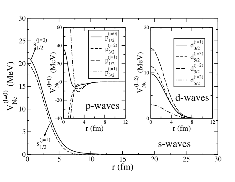
Figure 1: Neutron-³H potentials for the different $\ell_{j_{N}}^{(j)}$ waves corresponding to the parameters in table 1. The external panel shows the two $s$-wave potentials, and the internal panels show the four $p$-wave (left), and the four $d$-wave (right) neutron-³H potentials, respectively.

Using a gradient minimization method we have found the strengths and ranges of the Gaussian potentials given in table 1. In Fig.1 we plot the corresponding ³H-neutron potentials for the different $\ell_{j_{N}}^{(j)}$ states. The $s$-wave potentials are repulsive, which is consistent with population by two protons or neutrons of the two $s_{1/2}$ states in ³He or ³H, respectively. As a consequence the third proton in ⁴Li, or the third neutron in ⁴H, can not populate these $s$-states due to the Pauli principle. The potentials for the $d$-states are also repulsive, pushing up the energies of the $d_{5/2}$ and $d_{3/2}$ states. This is also expected but for a different reason, i.e. the $d$-states should be higher in energy than the states in the $p$ shell, and therefore with a smaller probability of being populated by the valence nucleon.

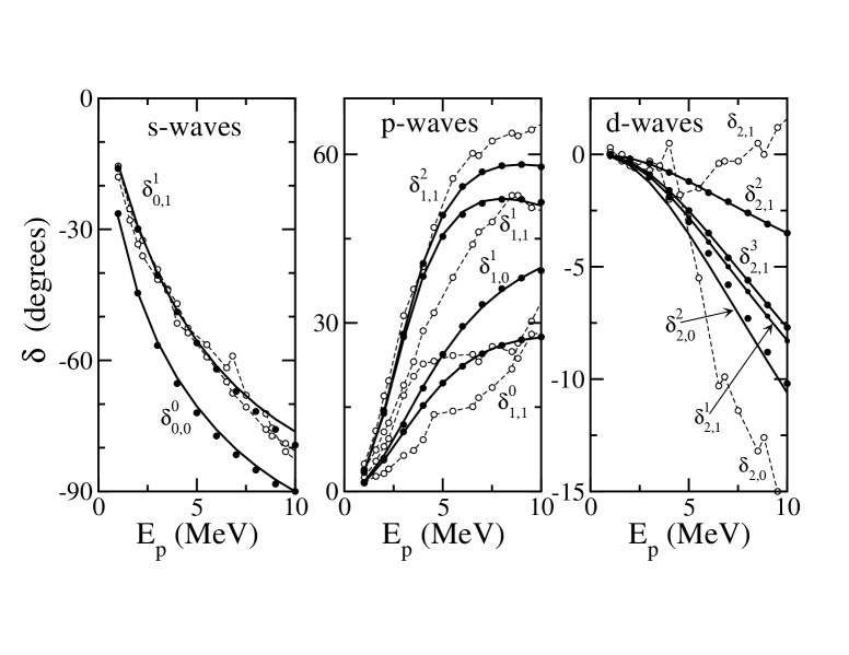
Figure 2: Computed phase shifts $\delta_{\ell,s}^{j}$ (solid lines) for the $s$-wave (left), $p$-wave (center), and $d$-wave (right) ³He-proton potentials using the parameters given in table 1. The solid circles show the experimental phase shifts in [31], and the open circles (connected with dashed curves) are the experimental data from [30]. In the right part of the figure the solid circles correspond to $\delta_{2,0}^{2}$ from [31] but with opposite sign.

In Fig.2 we show the computed phase shifts (solid lines) for the different $s$, $p$ and $d$-wave ³He-proton potentials. The agreement with the experimentally derived phase shifts in [31] (black circles) is very good. For comparison we also show (open circles) the experimental phase shifts given in [30]. To guide the eye we have connected these data with dashed curves. These data [30] are not fully consistent with the ones given in [31], although the global behaviour is similar. Also, in [30] the $d$-wave phases are assumed to be degenerate (denoted $\delta_{2,0}$ and $\delta_{2,1}$ in the right part of Fig.2) with a resulting erratic dependence on the energy.

The present numerical fit for $d$-waves only used the experimental $\delta_{2,1}^{1}$, $\delta_{2,1}^{2}$, and $\delta_{2,1}^{3}$ phase shifts, since the numerical method was unable to find a potential matching simultaneously all four sets of $d$-wave shifts in [31]. As seen in the right part of Fig.2 the match of the three sets of experimental phase shifts used for the numerical fit (black circles) is excellent. The lowest solid line shows the $\delta_{2,0}^{2}$ phase shifts obtained with the potential parameters fitting the other three sets. It is puzzling that these phase shifts are in almost perfect agreement with those in [31], provided the sign is reversed (black points). In any case these computed $\delta_{2,0}^{2}$ phase shifts exhibit the same global behaviour (negative and decreasing with a similar rate) as those of [30] (open circles).

We have also tried to fit the experimental ³He-proton phase shifts [31] with the potential in Eq.(5), even though the conserved quantum numbers then are inappropriate. The numerical procedure fails dramatically in determining the potential parameters for the $p$ and $d$-waves in this case. The same failure appears with other analytical expressions for the radial form factors. It is certainly very difficult (if not impossible) to construct a potential like Eq.(5) reproducing the experimental ³He-proton phase shifts. In total, this demonstrates that the experimental phase shifts are inconsistent with Eq.(5), but consistent with Eq.(6).

3 ⁴H properties.

The structure of ⁴H is obtained from the neutron-³H potentials given in table 1 and plotted in Fig.1. Only the potentials in the $p_{3/2}$ and $p_{1/2}$ states exhibit attractive pockets with barriers. These states are therefore the only ones which might support two-body resonances. The central $p$-wave potential contains two Gaussians with slightly different ranges and almost identical strengths of opposite sign, which is an attractive surface central potential. We test the dependency on two choices of the Coulomb interaction corresponding to Gaussian and point-like ³He-charge distributions. The result in table 1 for the point-like Coulomb potential is almost identical to that of a Gaussian charge distribution. The fits to the data are equally good. With artificially small errors of 0.1 degrees on all phase shift data points the $\chi^{2}$ per data is around 8. This means that an error of 1 degree would give a $\chi^{2}$ per data point equal to about 0.08.

Table 2: Resonance energies and widths $(E_{R},\Gamma_{R})$, in MeV, in ⁴H. The 2^nd and 3^rd columns are the results obtained as poles of the $S$-matrix in this work and in [15]. The 4^th column gives the results from this work assuming that the resonances energies correspond to a maximum of $\frac{d\delta}{dE}$ (and $\Gamma_{R}$=$2/\left(\frac{d\delta}{dE}\right)_{max}$). The last two columns are the experimental values from [28] and [9], where an $R$-matrix fit or a Breit-Wigner fit to the peak of the experimental cross sections is made. In [9] the energies are given without spin-parity assignment.

$J^{\pi}$	This work	[15]	This work	[28], exp.	[9], exp.
	$S$-matrix poles	$S$-matrix poles	$\left({d\delta}/{dE}\right)_{max}$	$R$-matrix	Breit-Wigner
	$(E_{R},\Gamma_{R})$	$(E_{R},\Gamma_{R})$	$(E_{R},\Gamma_{R})$	$(E_{R},\Gamma_{R})$	$(E_{R},\Gamma_{R})$
2-	(1.22,3.34)	(1.52,4.11)	(1.80,6.21)	(3.19,5.42)	(1.6,$\sim$0.8)
1-	(1.15,3.49)	(1.23,5.80)	(1.70,6.84)	(3.50,6.73)	(3.4,$\sim$0.8)
0-	(0.77,6.72)	(1.19,6.17)	(1.92,19.1)	(5.27,8.92)	(6.0,$\sim$1.0)
1-	(1.15,6.38)	(1.32,4.72)	(2.25,14.6)	(6.02,12.99)	—

The $p$-wave potentials give rise to four resonant states in ⁴H, whose energies and widths are given in the second column of table 2. These states have been obtained as poles of the $S$-matrix and agree rather well with the ones found in [15] (third column), where resonances are also computed as poles of the $S$-matrix, and where a different procedure (resonating group method) is used to build the neutron-triton interaction.

There is a clear disagreement between the theoretical energies and widths given in columns 2 and 3, and the experimental ones in column 5 [28]. However, the experimental data [28] have been obtained from a charge symmetric reflection of the $R$-matrix parameters for ⁴Li. It is well known, as explicitly written in [28], that the structure given by the $S$-matrix poles is quite different, giving rise to $p$-wave resonances occurring even in a different order. This fact is illustrated in [34], where large variations for the resonance parameters in ⁵He and ⁵Li are found depending on what procedure is used to extract them. In all cases the resonance energies obtained as poles of the $S$-matrix are clearly lower than the ones obtained using a conventional $R$-matrix analysis. This is particularly important for broad resonances.

A recent Breit-Wigner fit [9] of the experimental missing-mass spectra suggests that the ground state energy of ⁴H is a factor of two lower than in [28] (last column in table 2). The widths of all the states are also much smaller than the ones given in [28]. In [9] only the energies and widths are given, without the spin and parity assignment.

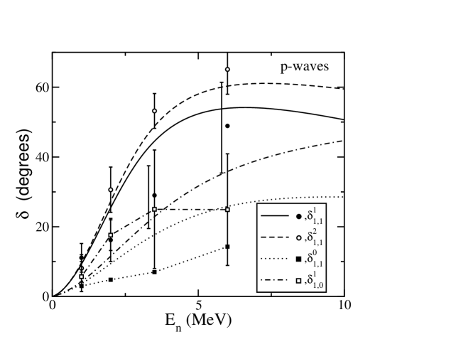
Figure 3: Computed phase shifts $\delta_{\ell,s}^{j}$ for the $p$-wave neutron-³H potential using the parameters given in table 1. The experimental data (solid circles for $\delta_{1,1}^{1}$, open circles for $\delta_{1,1}^{2}$, solid squares for $\delta_{1,1}^{0}$, and open squares for $\delta_{1,0}^{1}$) are from [29].

It is quite obvious that a direct comparison of the resonance energies for ⁴H obtained in this work as poles of the $S$-matrix with the ones obtained from the $R$-matrix or Breit-Wigner analyses (given in the last two columns of table 2) is not appropriate. This comparison can not be used to test the validity of the neutron-triton interaction. A more efficient way is to compare directly to the very few available experimental neutron-triton phase-shifts [29]. In Fig.3 we show the computed neutron-triton phase shifts ($\delta_{\ell,s}^{j}$) for the $p$-potentials in Fig.1. The solid, dashed, dotted, and dot-dashed curves correspond to the $\delta_{1,1}^{1}$, $\delta_{1,1}^{2}$, $\delta_{1,1}^{0}$, and $\delta_{1,0}^{1}$ phase shifts, respectively. The corresponding experimental data [29] are given by the solid circles, open circles, solid squares, and open squares, respectively. As seen in the figure, the error bars of the data are large. The $\delta_{1,1}^{0}$ data are only available without error bars, which presumably should be large. For $\delta_{1,1}^{0}$ and $\delta_{1,0}^{1}$ the experimental data have been connected with the same kind of curve as for the computed ones.

Using the parameters in table 1 to compute (not fit) the very few and uncertain neutron-triton phase shifts we arrive at an $\chi^{2}$ per data point equal to about 8, which is comparable to the ³He-proton fit. The neutron-triton phase shifts could easily be precisely reproduced with potentials of the form in eq. (6). However, the few and inaccurate points do not make that worthwhile. Instead we rely on the very precise fits of the ³He-proton phase shifts and the charge independence of the strong interaction.

As seen in Fig.3, the computed phase shifts agree reasonably well with the experiment. We can observe that neither the computed phase shifts nor the experimental ones cross the value $\pi/2$. The definition of resonances as the energy at which $\delta(E)$=$\pi/2$ is then not applicable here. This fact contradicts the results shown in [13], where the neutron-triton phase shifts do cross the value $\pi/2$. In fact, in [13] resonances are precisely defined as the energies where $\delta(E)$=$\pi/2$. This seems to disagree with the experimental data. The phase shifts in Fig.3 are consistent with the existence of broad resonances defined as the energies where $d\delta/dE$ has a maximum, and $\Gamma_{R}$=$2/\left(\frac{d\delta}{dE}\right)_{max}$ [35]. Following this prescription we obtain the energies and widths given in the fourth column of table 2. The different states are now reordered, and the new energies and widths are significantly larger than the ones obtained as poles of the $S$-matrix.

The $R$-matrix analysis of these experimental phase shifts [29] leads to a $2^{-}$ ground state energy for ⁴H of 3.4 MeV with a width of 5.5 MeV. Therefore, since our neutron-triton interaction agrees reasonably well with the experimental phase shifts [29], the resonance energies and widths obtained as poles of the $S$-matrix and given in the second column of table 2, are consistent with the $R$-matrix analysis which gives the ground state energy slightly above 3 MeV.

The $s$-wave potential given in table 1 gives rise to singlet and triplet scattering lengths equal to 5.32 fm and 3.01 fm, respectively, in agreement with the experimental values of 4.98$\pm$0.29 fm and 3.13$\pm$0.11 fm, respectively [36]. Thus mirror symmetry seems to be rather well fulfilled.

4 Results for ⁵H

Once the two-body interactions are fixed, we investigate the low-energy spectrum of ⁵H. As discussed above only the attractive $p$-waves can be responsible for low-lying states. The resulting angular momentum and parity, $J^{\pi}$, of these three-body states are then expected to be 1/2⁺, 3/2⁺, and 5/2⁺ states. The Pauli principle prohibits larger $J$-values with positive parity. Negative parity states must involve one neutron-triton $p$-level and one of either $s$ or $d$-character. These three-body states are necessarily then situated at higher energies if they appear at all. For each $J^{\pi}$, we first solve the angular part of the (complex rotated) Faddeev equations, which provide the effective potentials in the radial equations. As a second step we solve the radial equations that give the radial wave functions and the energies for each of the states.

4.1 Angular part.

To solve the angular part of the Faddeev equations, the angular eigenfunctions $\phi_{n}^{(i)}$ in Eq.(2) are expanded in terms of the complete basis $\left\{[Y_{\ell_{x}\ell_{y}}^{KL}\otimes\chi_{s_{x},s_{y}}]^{J}\right\}$, where the hyperspherical harmonics $Y_{\ell_{x}\ell_{y}}^{KL}$ are the free solutions with only the kinetic energy operator and $\chi_{s_{x},s_{y}}$ is the spin wave function. For each Jacobi set $\ell_{x}$ and $\ell_{y}$ are the orbital angular momenta associated to the Jacobi coordinates $x$ and $y$, $s_{x}$ is the coupling of the spins of the two particles connected by $x$, $L$ and $S$ are the total orbital angular momentum and spin, respectively, and $J$ is the total angular momentum of the three-body system. In this expansion convergence is required at two different levels. First, the basis containing all contributing partial wave components $\{\ell_{x},\ell_{y},L,s_{x},S\}$ must be included in the expansion, and second, for each component, the maximum value, $K_{max}$, of the hypermomentum $K$ must be large enough to ensure convergence for all necessary distances.

Table 3: The largest partial wave components included in the calculation for the 1/2⁺ state of ⁵H. The left and right parts refer to the Jacobi sets where $x$ connects the two neutrons, or the core and one of the neutrons, respectively. The sixth row gives the maximum value of the hypermomentum $K$ used for each of these components. The last row gives the contribution of the component to the total norm of the (complex rotated) wave function. Only those components contributing more than 1% are given.

$l_{x}$	0	1	1	2	0	0	1	1	1	1
$l_{y}$	0	1	1	2	0	0	1	1	1	1
$L$	0	1	1	0	0	0	0	0	1	1
$s_{x}$	0	1	1	0	0	1	0	1	0	1
$S$	0.5	0.5	1.5	0.5	0.5	0.5	0.5	0.5	0.5	1.5
$K_{max}$	180	82	102	84	80	100	182	182	82	82
$W$ (5H)	92.2	2.0	3.7	1.9	2.6	8.3	21.0	62.4	1.6	3.8

Table 4: The same as table 3 for the 3/2⁺ state of ⁵H

$l_{x}$	0	1	1	2	1	1	1	1	1	2
$l_{y}$	2	1	1	0	1	1	1	1	1	0
$L$	2	1	1	2	1	1	1	2	2	2
$s_{x}$	0	1	1	0	0	1	1	0	1	1
$S$	0.5	0.5	1.5	0.5	0.5	0.5	1.5	0.5	0.5	0.5
$K_{max}$	182	82	122	122	82	82	122	122	182	82
$W$ (5H)	43.8	5.0	20.1	30.6	3.8	1.3	19.6	18.2	52.6	4.0

The 1/2⁺, 3/2⁺, and 5/2⁺ states in ⁵H have been calculated including all the possible components involving $s$, $p$, and $d$-waves. A $K_{max}$ value of at least 60 has been used, except for the largest components where $K_{max}$ has been increased to guarantee convergence of the effective potentials. In tables 3, 4, and 5 we specify the quantum numbers, including the $K_{max}$ values, of the largest components for each of the states computed.

Table 5: The same as table 3 for the 5/2⁺ state of ⁵H

$l_{x}$	0	1	2	1	1	1	2	2
$l_{y}$	2	1	0	1	1	1	0	0
$L$	2	1	2	1	2	2	2	2
$s_{x}$	0	1	0	1	0	1	0	1
$S$	0.5	1.5	0.5	1.5	0.5	0.5	0.5	0.5
$K_{max}$	182	82	122	82	122	182	82	82
$W$ (5H)	55.1	13.1	31.4	12.7	19.9	60.1	1.8	5.2

Solving now the angular eigenvalue equation we obtain the eigenvalues, $\lambda_{n}(\rho)$, needed to construct the effective potentials in the radial equations. In particular, it turns out that it is sufficient to use a scaling angle of $\theta$=0.35 rads for the $1/2^{+}$ and $3/2^{+}$ states, and 0.30 rads for the 5/2⁺ state, respectively.

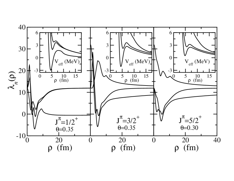
Figure 4: Real parts of the three lowest angular eigenvalues $\lambda(\rho)$ (external plots) and the effective hyperradial potentials $V_{eff}=\hbar^{2}(\lambda+15/4)/(2m\rho^{2})$ (insets) for the 1/2⁺, 3/2⁺ and 5/2⁺ states of ⁵H as a function of $\rho$.

In Fig.4 we show the three most contributing eigenvalues $\lambda(\rho)$ for each of the 1/2⁺, 3/2⁺ and 5/2⁺ states in ⁵H. For the sake of clarity, we only show the real parts, which for short-range interactions must reproduce the hyperspherical spectrum ($K(K+4)$) at $\rho=0$ and $\rho=\infty$ [23]. The most attractive pocket appears for the 1/2⁺ state, which therefore is expected to be the ground state, in agreement with the experimental results. This is seen more clearly in the insets, which show the real parts of the effective radial potentials, $V_{eff}=(\lambda+15/4)/\rho^{2}$. Together with the attractive pockets one can observe a series of potential barriers that might be able to hold three-body resonances.

4.2 Energies and wave functions.

As a final step, we now solve the coupled set of differential radial equations for states with $1/2^{+}$, $3/2^{+}$, and $5/2^{+}$. Five adiabatic effective potentials are included in the calculations. Resonances are then found searching for radial solutions behaving asymptotically as the outgoing waves specified in Eq.(4). To impose this analytically known asymptotic behaviour is not strictly necessary. The complex rotated resonance wave functions are actually falling off exponentially, and a simple box boundary condition would then be sufficient to obtain the correct solutions. However this boundary condition is numerically much more delicate, since the effective potentials have to be computed accurately at much larger distances than those required by the analytic boundary condition.

Table 6: Resonance energies and widths $(E_{R},\Gamma_{R})$, in MeV, for the $1/2^{+}$, $3/2^{+}$, and $5/2^{+}$ states in ⁵H for the Gaussian three-body effective potential with the range $b_{3b}=3$ fm and three different strengths $S_{3b}$ given in MeV in the first row. The last column shows the results with $S_{3b}=-30$ MeV when only $s$ and $p$-waves are included.

$S_{3b}$	$-25$	$-30$	$-35$	$-30(s,p)$
$1/2^{+}$	(1.69, 1.95)	(1.57, 1.53)	(1.40, 1.11)	(1.55, 1.35)
$3/2^{+}$	(3.24, 4.31)	(3.25, 3.89)	(3.23, 3.44)	(3.05, 3.46)
$5/2^{+}$	(2.85, 3.13)	(2.82, 2.51)	(2.68, 1.83)	(2.65, 2.00)
$5/2^{+}$				(3.70, 4.31)

Table 7: Resonance energies and widths $(E_{R},\Gamma_{R})$, in MeV, for the $1/2^{+}$, $3/2^{+}$, and $5/2^{+}$ states in ⁵H for the Gaussian three-body effective potential with strength $S_{3b}=-30$ MeV and four different ranges $b_{3b}$ given in fm in the first row.

$b_{3b}$	$2.95$	$3.00$	$3.05$	$3.15$
$1/2^{+}$	(1.63, 1.70)	(1.57, 1.53)	(1.51, 1.37)	(1.36, 1.05)
$3/2^{+}$	(3.26, 4.09)	(3.25, 3.89)	(3.23, 3.69)	(3.17, 3.26)
$5/2^{+}$	(2.86, 2.75)	(2.82, 2.51)	(2.76, 2.26)	(2.62, 1.79)

We estimate the range, $b_{3b}$, of the effective Gaussian three-body potential, $V_{3b}=S_{3b}e^{-\rho^{2}/b_{3b}^{2}}$, to be around 3.0 fm which is the hyperradius corresponding to a configuration where all the three particles are touching each other. In table 6 we give the corresponding computed resonances in ⁵H for different strengths varying around the value $-30$ MeV which places the lowest resonance energy close to the measured values. The main effect of decreasing the three-body attraction is to increase the width of the resonances, while the energies only increase moderately. A further decrease of attraction produce $3/2^{+}$ and $5/2^{+}$ resonances too broad to appear for the scaling angles used in the calculation.

Similar effects are observed when the range of the three-body potential is changed. The results shown in table 7 correspond to a three-body force with a fixed strength $S_{3b}=-30$ MeV and four different values of the three-body range $b_{3b}$. Again the main effects are observed in the width of the resonances. A decrease of $b_{3b}$ gives rise to larger resonance energies and widths, but a change of 0.2 fm in the range modifies the energies by at most 0.27 MeV, while the widths change between 0.7 MeV and 1 MeV for all cases. Smaller values of $b_{3b}$ produce 3/2⁺ and 5/2⁺ resonances too broad to be obtained with the complex scaling angles used in the calculation. From tables 6 and 7 we conclude that the ground state of ⁵H is a 1/2⁺ resonance. If the energy is adjusted to be around 1.6 MeV, the two excited states, 3/2⁺ and 5/2⁺, appear about 1.65 MeV and 1.25 MeV higher, respectively.

To test the role played by the $d$-waves, we show in the last column of table 6 the energies and widths of the resonances when the two-body $d$-wave potentials vanish. A strength $S_{3b}=-30$ MeV has been used for the three-body force in this case. Inclusion of the $d$-wave interactions only marginally changes the structures. The variation in the energies and widths is certainly visible, and especially the widths increase by including the $d$-waves. In fact, when the $d$-wave interactions are zero a second $5/2^{+}$ resonance appears at about 3.70 MeV. With $d$-waves this resonance is too broad to be obtained with the scaling angle $\theta=0.30$ rads used in this calculation.

Figure 5: Real parts of the rotated radial wave functions for the 1/2⁺ state (left), the 3/2⁺ state (middle) and the 5/2⁺ state (right) in ⁵H with a rotation angle $\theta$. We show the computed wave functions that contribute most (thick lines) and the asymptotic functions $\sqrt{\rho}H_{K+2}^{(1)}(|\kappa|\rho e^{i(\theta-\theta_{R})})$ (thin lines), see Eq. (4).

For the three resonances, the radial wave functions associated with the three lowest effective potentials given in Fig.4 are shown by the thick curves in Fig.5. The wave functions have been obtained with a three-body force with Gaussian parameters $S_{3b}=-30$ MeV and $b_{3b}=3.0$ fm. To keep the figure cleaner only the real parts are shown. As expected, after complex scaling, the resonance radial wave functions are approaching zero according to the asymptotics given in Eq.(4), which is shown in the figure by the thin curves. In all cases the computed wave functions have reached the expected asymptotic behavior already at about 40 fm.

Since the complex rotated three-body wave functions can be normalized, we compute the relative weights of the different components given in the last rows of tables 3, 4, and 5. When the three-body wave functions are written in the first Jacobi set ($x$ between the two neutrons) the $1/2^{+}$ ground state is clearly dominated by the $\ell_{x}=\ell_{y}=L=0$ component (more than 90% of the norm), while the $sd$ interferences ($L=2$) are the dominating components for the excited $3/2^{+}$ and $5/2^{+}$ states (75% and 85% of the norm, respectively). In the second and third Jacobi sets ($x$ from ³H to one of the neutrons) the $\ell_{x}=\ell_{y}=1$ components dominate in all the three cases, whereas the coupling to the total $L$ must produce the same distribution in all Jacobi systems, i.e. $L=0$ and $L=2$ for ground and excited states, respectively. Also the total spin $S$ is conserved in transformations between Jacobi systems.

4.3 Comparison with other computed and measured results

Table 8: Theoretical and experimental energies ($E_{R}$) and widths ($\Gamma_{R}$) for the 1/2⁺, 3/2⁺ and 5/2⁺ resonances in ⁵H. The results correspond to the references quoted in the first column. The first, second and third rows show our results, respectively for our full interaction (with $S_{3b}=-30$ MeV $b_{3b}=3$ fm), when the $d$-wave interactions are zero, and with the ³H-neutron potential given in [16].

$(E_{R},\Gamma_{R})$ (MeV)
$J^{\pi}$	1/2+	3/2+	5/2+
5H(full)	(1.57,1.53)	(3.25,3.89)	(2.82,2.51)
5H($d=0$)	(1.55,1.35)	(3.05,3.46)	(2.65,2.00)
			(3.70,4.31)
Theor. [16]	(2.26,2.93)	(4.41,6.22)	(2.58,1.78)
			(3.81,4.70)
Theor. [12]	(2.5-3.0,3-4)	(6.4-6.9,8)	(4.6-5.0,5)
Theor. [13]	(3.0-3.2,1-4)	(–,–)	(–,–)
Theor. [15]	(1.59,2.48)	(3.0,4.8)	(2.9,4.1)
Exp. [3]	($1.7\pm 0.3$,$1.9\pm 0.4$)	(–,–)	(–,–)
Exp. [8]	($1.8\pm 0.1$,$<0.5$)	(–,–)	($2.7\pm 0.1$,$<0.5$)
Exp. [4]	(1.8,1.3)	($>2.5$,–)	($>2.5$,–)
Exp. [5]	(2,2.5)	($>2.5$,–)	($>2.5$,–)
Exp. [6]	(3,6)	(–,–)	(–,–)
Exp. [9]	($5.5\pm 0.2$,$5.4\pm 0.6$)	($>10$,$>2$)	($>10$,$>2$)

We compare our results in the first row of table 8 to different theoretical an experimental values extracted from the literature. The results given in the third row correspond to the resonances obtained by following the same method as described in this work, but using the ³H-neutron interaction given in ref.[16]. This potential is used in [12] to obtain the ⁵H-resonances (fourth row) after solving the Schrödinger equation by means of a hyperspherical harmonics expansion of the wave function. It is not clear whether $d$-wave interactions are included in the calculations in ref.[12]. For this reason the results in the second and third rows of table 8 omitted $d$-waves. We then observe that the results given in the third and fourth rows are distinctly different, even if similar two-body potentials are used in both cases. This is due to the fact that in [12] resonances are determined from the observed rapid variations in the phase shifts as a function of the energy, while we obtain them as poles of the $S$-matrix. The definition as $S$-matrix poles usually gives lower energies and smaller widths. In any case the potential used in [12] is producing a ground state at an energy significantly higher than with the potential used in this work, and in fact not very far from the energy of the $5/2^{+}$ state. We emphasize that the potential in [16] has the form in Eq.(5), that we have found to be inconsistent with the available ³H-neutron and ³He-proton experimental data.

In [13] also a phase shift analysis is employed to get the three-body resonances, and again the energy obtained for the ground state is roughly a factor of two higher than obtained in the present work. It is remarkable that our energies agree very well with those of [15], where a microscopic model combined with complex scaling is used to obtain resonances as poles of the $S$-matrix. However, our widths are systematically smaller than those of [15]. This has to be attributed to either different interactions or contributions from the triton-core. Among the different available experimental data, only [9] clearly disagree with our results. On the other hand, for most of the cases, the agreement between our theoretical energies and widths and the experimental values is quite good [3, 4, 5, 8].

5 Energy distributions

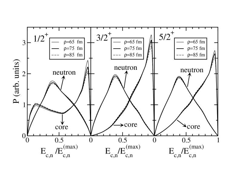
Figure 6: Energy distributions of the ³H-core and the neutrons after decay of the 1/2⁺ (left), 3/2⁺ (center), and 5/2⁺ (right) three-body resonances in ⁵H. The convergence of the results is illustrated by the different (almost overlapping) curves, which correspond to calculations with $\rho_{max}$ values of 65 fm (thin solid), 75 fm (thick solid), and 85 fm (dashed).

Recently we presented a method to compute the energy distributions of particles emerging from a three-body decay of a many-body resonance [37, 38]. The method exploits the fact that hyperspherical harmonics transform into themselves after Fourier transformation. Therefore the kinetic energy distribution of the fragments after decay of the resonance is, except for a phase-space factor, obtained as the absolute square of the total wave function in coordinate space for a large value of the hyperradius, but where the five hyperangles are interpreted as in momentum space [38].

After integration over the four hyperangles describing the directions of the two Jacobi momenta, $\mbox{\boldmath$k$}_{x}$ and $k_{y}$, conjugate to $x$ and $y$, the probability distribution as function of $k_{y}^{2}$ ($k_{y}^{2}\propto\cos^{2}\alpha$, where $\alpha$ is the fifth momentum hyperangle) is given by

$$P(k_{y}^{2})\propto P(\cos^{2}\alpha)\propto\sin(2\alpha)\int d\Omega_{x}d\Omega_{y}|\Psi(\rho_{max},\alpha,\Omega_{x},\Omega_{y})|^{2}\;,$$ (7)

where $\rho_{max}$ refers to a large value of the hyperradius where the asymptotic behaviour of the three-body wave function has been reached. Except for mass factors, $k_{y}$ is the momentum of the third particle relative to the three-body center of mass. Therefore the kinetic energy of the third particle is proportional to $k_{y}^{2}$ (or to $\cos^{2}\alpha$), and its energy distribution is then as given in Eq.(7). In particular, $\cos^{2}\alpha$ gives the energy of the particle relative to its maximum possible energy in the decay process.

This procedure has formally the shortcoming that the hyperradius $\rho_{max}$ in principle should be asymptotically large (since the detection takes place at large distance), and the larger the value of $\rho_{max}$ the larger the size of the required basis for the hyperspherical expansion. For short-range potentials the asymptotic limit is known to be the hyperspherical harmonics, reflected in the corresponding hyperharmonic spectrum of the hamiltonian without interaction. It was shown in previous reports [38] that the correct asymptotic limit is reached already at intermediate distances where the basis size is still manageable in the numerical calculations. An increase of $\rho_{max}$ requires a larger basis which then would reproduce the energy distribution found at the smaller distance with the smaller basis size. This optimum region of hyperradii is determined as the region where the observable is independent of $\rho_{max}$-variations; further increase of $\rho_{max}$ is not productive. Clearly this is a satisfactory procedure for short-range interactions.

Following this procedure we have computed the energy distributions of the fragments after decay of the ⁵H-resonances. The results for the 1/2⁺, $3/2^{+}$, and $5/2^{+}$ states are shown in the left, central, and right parts of Fig.6. Neutron and triton energy distributions are shown as a function of the corresponding particle energy relative to its maximum energy. Convergence has been tested by comparing calculations for three different values of $\rho_{max}$ (65 fm, 75 fm, and 85 fm) in Eq.(7). As seen in the figure all three calculations provide almost overlapping curves.

For the 1/2⁺ resonance (left part of Fig.6), the neutron energy distribution has an irregular broad peak at intermediate energies. The triton energy distribution has one peak very close to the maximum energy and a broader peak at low energies. This pattern corresponds to two types of decay mechanisms. The first is emission of ³H followed by decay of an intermediate two-neutron structure. This sequential decay amounts to a two-body process where the ³H-core receives maximum energy and the two neutrons move together in the opposite direction relative to the core. In the subsequent decay each neutron then must share the remaining energy which leads to an intermediate energy between zero and the maximum value. The existence of a low-lying neutron-neutron virtual $s$-state appears to be decisive in the decay process, even if a stable intermediate configuration of two neutrons does not exist, neither as bound states nor as resonances.

The second decay structure with the small triton energy corresponds to emission of two neutrons in opposite directions while the triton essentially remains at rest in the center. The two neutrons then share the available energy leading to intermediate energies for each of them. Combining these two mechanisms produces the computed irregular broad single-neutron peak.

For the $3/2^{+}$ and $5/2^{+}$ states (central and right parts of Fig.6) similar distributions are found for the neutrons except that they tend to be slightly more narrow. In contrast the triton energy distribution only has the high energy peak corresponding to the sequential decay of triton emission. The low-energy triton peak is not present because it is unfavorable for two neutrons to be far apart with a $d$-wave describing their center of mass motion.

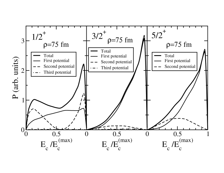
Figure 7: Contribution from the three adiabatic potentials in Fig.4 to the triton energy distributions after decay of the 1/2⁺ (left), 3/2⁺ (center), and 5/2⁺ (right) three-body resonances in ⁵H. The thick solid curve gives the total distributions, while the thin solid, thin dashed and thin dot-dashed curves give the individual contributions from the first, second, and third adiabatic potentials, respectively. In the right part of the figure the contribution from the third adiabatic potential is not visible.

In Fig.7 we show, for the three computed ⁵H resonances, the individual contributions to the triton energy distributions from the three adiabatic potentials shown in Fig.4. In the 5/2⁺ case the contribution from the third potential is not visible. The results in the figure correspond to $\rho_{max}=75$ fm. In all the three cases the main features of the total distribution (thick solid line) are produced by a single adiabatic potential (the second one for 1/2⁺, and the first one for 3/2⁺ and 5/2⁺). In particular these potentials are responsible for the two peaks at high and small triton energies in the 1/2⁺ case (left), and for the high energy peaks in the 3/2⁺ (center) and 5/2⁺ cases (right).

In the three cases, at $\rho=75$ fm, the angular eigenfunctions associated to this adiabatic potential is almost 100% given by the components in the second columns of tables 3, 4, and 5, respectively. These components correspond to a relative $s$-wave between the two neutrons. However, while in the 1/2⁺ case the triton is also in a relative $s$-wave relative to the two-neutron center of mass, in the 3/2⁺ and 5/2⁺ cases the triton is in a relative $d$-wave. This fact inhibits the appearance of the low energy peak in the triton energy distribution in the 3/2⁺ and 5/2⁺ cases. For the next most relevant adiabatic potential (the first one for 1/2⁺, and the second one for 3/2⁺ and 5/2⁺), the contribution comes also from the $\{\ell_{x}=\ell_{y}=L=0,S=1/2\}$ component in the 1/2⁺ case, but for the 3/2⁺ and $5/2^{+}$ states it comes from the $\{\ell_{x}=\ell_{y}=L=1,S=3/2\}$ component ($x$ between the neutrons).

6 Summary and conclusions

The hyperspheric adiabatic expansion method is used to investigate ⁵H in a three-body model where the ³H-core is surrounded by two neutrons. Three-body resonances are computed as poles of the $S$-matrix. We use the complex scaling method, which provides resonances as solutions of the Faddeev equations with complex energy and wave functions falling off exponentially at large distances.

The two-body ³H-neutron interaction is built with central, spin-orbit, and spin-spin terms, where each of the radial form factors is a sum of two Gaussians. The strengths and ranges of the Gaussians are adjusted to fit the available ³He-proton experimental data. These data are more reliable and abundant than the ³H-neutron data, and should lead to an appropriate ³H-neutron potential simply by switching off the Coulomb interaction. We have found that the experimental ³He-proton phase shifts can be reproduced only when the spin operators in the two-body potential are such that the mean field angular momentum quantum numbers are conserved quantum numbers for the valence nucleon. Use of such proper spin operators appears to be essential in a reliable description.

The ground state of ⁵H is found to have spin and parity $1/2^{+}$, and for an energy of around 1.6 MeV the width is about 1.5 MeV. Two excited states are then found at 2.8 MeV and 3.2 MeV, with spin and parity $5/2^{+}$ and $3/2^{+}$, respectively. Thus these states are broad and overlapping. The effective three-body force has a range corresponding to three touching particles. Then it modifies mainly the width of the resonances, keeping the energies rather stable. The agreement of these results with most of the available experimental data is remarkable.

For all the three states the dominating components correspond to a relative $s$-wave between the two neutrons. In the ground state this $s$-wave combines with another relative $s$-wave between the core and the center of mass of the two neutrons, while for the excited states it combines with a $d$-wave. In the second and third Jacobi sets the dominating components correspond to relative $p$-waves between the core and one of the neutrons as well as between the second neutron and the center of mass of ⁴H. Finally, we have found that the $1/2^{+}$ resonance decays with roughly equal probabilities through two-body sequential decay by ³H-emission and three-body decay by emission of the two neutrons in opposite directions. The $3/2^{+}$ and $5/2^{+}$ resonances only decay by triton emission. Both neutron and triton energy distributions are needed simultaneously to interpret these decay modes.

In conclusion, the three-body model describes efficiently the cluster structure of ⁵H as two neutrons and a triton. The resonances found are consistent with the experimental data. To get a good agreement with the experimental values in both ⁵H and ⁴H, the two-body neutron-triton interaction must have the spin dependence consistent with the mean field angular momentum quantum numbers of the triton. The decay leads to relatively broad energy distributions dominated by triton emission.

References

- [1] A.S. Jensen, K. Riisager, D.V. Fedorov and E. Garrido, Rev. Mod. Phys. 76 (2004) 215.
- [2] L.V. Grigorenko, Eur. Phys. J. A20 (2004) 419.
- [3] A.A. Korsheninnikov et al., Phys. Rev. Lett. 87 (2001) 092501.
- [4] M.S. Golovkov et al., Phys. Rev. C72 (2005) 064612.
- [5] G.M. Ter-Akopian et al., Eur. Phys. J. A25 (2005) 315.
- [6] M. Meister et al., Phys. Rev. Lett. 91 (2003) 162504.
- [7] M. Meister et al., Nucl. Phys. A723 (2003) 13.
- [8] S. I. Sidorchuk et al., Nucl. Phys. A719 (2003) 229c.
- [9] Yu.B. Gurov et al., Eur. Phys. J. A24 (2005) 231.
- [10] D.V. Aleksandrov, E.Yu. Nikol’skii, B.G. Novatskii, and D.N. Stepanov, Proceedings of the International Conference on Exotic Nuclei and Atomic Masses, Arles, France (1995) p.329.
- [11] G.F. Filippov, A.D. Bazavov, K. Kato, Phys. At. Nucl. 62 (1999) 1642.
- [12] N.B. Shul’gina, B.V. Danilin, L.V. Grigorenko, M.V. Zhukov and J.M. Bang, Phys. Rev. C62 (2000) 014312.
- [13] P. Descouvemont and A. Kharbach, Phys. Rev. C63 (2001) 027001.
- [14] N.K. Timofeyuk, Phys. Rev. C65 (2002) 064306.
- [15] K. Arai, Phys. Rev. C68 (2003) 034303.
- [16] N.B. Shul’gina, B.V. Danilin, V.D. Efros, J.M. Bang, J. S. Vaagen and M.V. Zhukov, Nucl. Phys. A597 (1996) 197.
- [17] L.V. Grigorenko, N.K. Timofeyuk, and M.V. Zhukov, Eur. Phys. J. A19 (2004) 187.
- [18] N. Tanaka, Y. Suzuki, and K. Varga, Phys. Rev. C56 (1997) 562.
- [19] Y.K. Ho, Phys. Rep. 99 (1983) 1.
- [20] N. Moiseyev, Phys. Rep. 302 (1998) 212.
- [21] E. Nielsen, D.V. Fedorov, A.S. Jensen and E. Garrido, Phys. Rep. 347 (2001) 373.
- [22] E. Garrido, D.V. Fedorov, and A.S. Jensen, Nucl. Phys. A708 (2002) 277.
- [23] D.V. Fedorov, E. Garrido, and A.S. Jensen, Few-body Systems 33 (2003) 153.
- [24] E. Garrido, D.V. Fedorov, and A.S. Jensen, Nucl. Phys. A733 (2004) 85.
- [25] E. Garrido, D.V. Fedorov, and A.S. Jensen, Eur. Phys. J. A25 (2005) 365.
- [26] E. Garrido, D.V. Fedorov, and A.S. Jensen, Phys. Rev. C69 (2004) 024002.
- [27] M.V. Zhukov, B.V. Danilin, D.V. Fedorov, J.M. Bang, I.J. Thompson and J.S. Vaagen, Phys. Rep. 231 (1993) 251.
- [28] D.R. Tilley and H.R. Weller and G.M. Hale, Nucl. Phys. A541 (1992) 1.
- [29] T.A. Tombrello, Phys. Rev. 143 (1966) 772.
- [30] T.A. Tombrello, Phys. Rev. 138 (1965) B40.
- [31] L. Beltramin, R. del Frate and G. Pisent, Nucl. Phys. A442 (1985) 266.
- [32] E. Garrido, D.V. Fedorov, and A.S. Jensen, Phys. Rev. C68 (2003) 014002.
- [33] L. Drigo and G. Pisent, Nuovo Cim. 70 (1970) 592.
- [34] A. Csótó and G.M. Hale, Phys. Rev. C55 (1997) 536.
- [35] J. Carlson, V.R. Pandharipande, and R.B. Wiringa, Nucl. Phys. A424 (1984) 49.
- [36] M.K. Jones et al., Phys. Rev. C42 (1990) R807.
- [37] D.V. Fedorov, H.O.U. Fynbo, E. Garrido, and A.S. Jensen, Few-body Systems 34 (2004) 33.
- [38] E. Garrido, D.V. Fedorov, A.S. Jensen and H.O.U. Fynbo, Nucl. Phys. A766 (2006) 74.