The hyperon-nucleon interaction: conventional versus effective field theory approach

Hyperon-nucleon interactions are presented that are derived either in the conventional meson-exchange picture or within leading order chiral effective field theory. The chiral potential consists of one-pseudoscalar-meson exchanges and non-derivative four-baryon contact terms. With regard to meson-exchange hyperon-nucleon models we focus on the new potential of the Jülich group, whose most salient feature is that the contributions in the scalar–isoscalar ($\sigma$) and vector–isovector ($\rho$) exchange channels are constrained by a microscopic model of correlated $\pi\pi$ and $K\overline{K}$ exchange.

1 Introduction

For several decades the meson-exchange picture provided the only practicable and systematic approach to the description of hadronic reactions in the low- and medium-energy regime. Specifically, for the fundamental nucleon-nucleon ($NN$) interaction rather precise quantitative results could be achieved with meson-exchange models MHE ; Mac01 . Moreover, utilizing for example ${\rm SU(3)}_{f}$ (flavor) symmetry or $G$-parity arguments, within the meson-exchange framework, interaction models for the hyperon-nucleon ($YN$) MRS89 ; Hol89 ; Reu94 ; YNN1 ; Rij99 ; Tom01 ; Hai05 ; Rij06 or nucleon-antinucleon ($N\overline{N}$) Kle02 systems could be constructed consistently. However, over the last 10 years or so a new powerful tool has emerged, namely chiral perturbation theory or, generally speaking, effective field theory (EFT). The main advantage of this scheme is that there is an underlying power counting that allows to improve calculations systematically by going to higher orders and, at the same time, provides theoretical uncertainties. In addition, it is possible to derive two- and corresponding three-body forces as well as external current operators in a consistent way. For reviews we refer to Bed02 ; Kap05 ; Epelbaum:2005pn .

Recently the $NN$ interaction has been described to a high precision using chiral EFT Epe05 (see also Entem:2003ft ). In that work, the power counting is applied to the $NN$ potential, as originally proposed by Weinberg Wei90 ; Wei91 . The $NN$ potential consists of pion exchanges and a series of contact interactions with an increasing number of derivatives to parameterize the shorter ranged part of the $NN$ force. A regularized Lippmann-Schwinger equation is solved to calculate observable quantities. Note that in contrast to the original Weinberg scheme, the effective potential is made explicitly energy-independent as it is important for applications in few-nucleon systems (for details, see Epe98 ).

Contrary to the $NN$ system, there are very few investigations of the $YN$ interaction using EFT. Hyperon and nucleon mass shifts in nuclear matter, using chiral perturbation theory, have been studied in Sav96 . These authors used a chiral interaction containing four-baryon contact terms and pseudoscalar-meson exchanges. Recently, the hypertriton and $\Lambda d$ scattering were investigated in the framework of an EFT with contact interactions only Ham02 . Korpa et al. Kor01 performed a next-to-leading order (NLO) EFT analysis of $YN$ scattering and hyperon mass shifts in nuclear matter. Their tree-level amplitude contains four-baryon contact terms; pseudoscalar-meson exchanges were not considered explicitly, but ${\rm SU(3)}_{f}$ breaking by meson masses was modeled by incorporating dimension two terms coming from one-pion exchange. The full scattering amplitude was calculated using the Kaplan-Savage-Wise resummation scheme Kap98 . The $YN$ scattering data were described successfully for laboratory momenta below 200 MeV, using 12 free parameters. Some aspects of strong $\Lambda N$ scattering in EFT and its relation to various formulations of lattice QCD are discussed in Beane:2003yx . Finally, in this context we note that first lattice QCD results on the $YN$ interaction have appeared Bea06 .

In this review we describe a a recent application of the scheme used in Epe05 to the $YN$ interaction by the Bonn-Jülich group Pol06 . Analogous to the $NN$ potential, at leading order (LO) in the power counting, the $YN$ potential consists of pseudoscalar-meson (Goldstone boson) exchanges and of four-baryon contact terms, where each of these two contributions is constrained via ${\rm SU(3)}_{f}$ symmetry. The results achieved by us within this approach are confronted with the available $YN$ data and they are also compared with predictions of a new conventional meson-exchange $YN$ model, developed likewise by the Jülich group Hai05 , whose most salient feature is that the contributions in the scalar–isoscalar ($\sigma$) and vector–isovector ($\rho$) exchange channels are constrained by a microscopic model of correlated $\pi\pi$ and $K\overline{K}$ exchange. Results of the Nijmegen $YN$ model NSC97f Rij99 are presented too.

The contents of this review are as follows. In Section 2 we discuss some general properties of the coupled $\Lambda N$ and $\Sigma N$ systems. We also introduce the coupled-channels Lippmann-Schwinger equation that is solved for obtaining the reaction amplitude. The effective potential in leading order chiral EFT is developed in Section 3. Here we first give a brief recollection of the underlying power counting for the effective potential and then investigate the ${\rm SU(3)}_{f}$ structure of the four-baryon contact interactions. The lowest order ${\rm SU(3)}_{f}$-invariant contributions from pseudoscalar meson exchange are derived too. Some general remarks about meson-exchange potentials of the $YN$ interaction are given in Section 4. We also provide a more specific description of the new meson-exchange potential of the Jülich group Hai05 , where we focus on the utilized model of correlated $\pi\pi$ and $K\overline{K}$ exchange. Results of both interactions for low-energy $YN$ cross sections are presented in Section 5. We show the empirical and calculated total cross sections, differential cross sections and give the values for the scattering lengths. Also, predictions for some $YN$ phase shifts are presented and results for binding energies of light hypernuclei are listed. The review closes with a summary and an outlook for future investigations.

2 The scattering equation

In the meson-meson and meson-baryon sector, chiral interactions can be treated perturbatively in powers of a low-energy scale (chiral perturbation theory). This is not the case for the baryon-baryon sector, otherwise there could be no bound states, such as the deuteron. Weinberg Wei91 realized that an additional scale arises from intermediate states with only two nucleons, which requires a modification of the power counting. He proposed to apply the techniques of chiral perturbation theory to derive an effective potential, $V$, and not directly the scattering amplitude. This effective potential is defined as the sum of all irreducible diagrams. The effective potential $V$ is then put into a Lippmann-Schwinger equation to obtain the reaction or scattering amplitude,

$$T=V+VGT\ ,$$ (1)

where $G$ is the non-relativistic free two-body Green’s function. Solving the scattering equation (1) also implies that the reaction amplitude $T$ fulfills two-body unitarity.

Treating the Lippmann-Schwinger equation for the $YN$ system is more involved than for the $NN$ system. Since the mass difference between the $\Lambda$ and $\Sigma$ hyperons is only about 75 MeV the possible coupling between the $\Lambda N$ and $\Sigma N$ systems needs to be taken into account. Moreover, for a sensible comparison of the results with experiments it is preferable to solve the scattering equation in the particle basis because then the Coulomb interaction in the charged channels can be incorporated. Here we use the method originally introduced by Vincent and Phatak Vin74 that was e.g. also applied in the EFT studies of the $NN$ interaction WME01 . Furthermore, the particle basis allows to implement the correct physical thresholds of the various $\Sigma N$ channels. To facilitate the latter aspect we also use relativistic kinematics for relating the total energy $\sqrt{s}$ to the c.m. momenta in the various $YN$ channels in the actual calculations, cf. Hai05 . Note that the interaction potentials themselves are calculated in the isospin basis.

The concrete particle channels that couple for a specific charge $Q$ are

$$Q=+2: \Sigma^{+}p$$

$$Q=+1: \Lambda p,\Sigma^{+}n,\Sigma^{0}p$$

$$Q=\phantom{+}0: \Lambda n,\Sigma^{0}n,\Sigma^{-}p$$

$$Q=-1: \Sigma^{-}n$$ (2)

Therefore, e.g., for $Q=0$ the quantities in Eq. (1) are then $3\times 3$ matrices,

$$V=\left(\begin{array}[]{ccc}V_{\Lambda n\to\Lambda n}&V_{\Lambda n\to\Sigma^{0}n}&V_{\Lambda n\to\Sigma^{-}p}\\ V_{\Sigma^{0}n\to\Lambda n}&V_{\Sigma^{0}n\to\Sigma^{0}n}&V_{\Sigma^{0}n\to\Sigma^{-}p}\\ V_{\Sigma^{-}p\to\Lambda n}&V_{\Sigma^{-}p\to\Sigma^{0}n}&V_{\Sigma^{-}p\to\Sigma^{-}p}\end{array}\right)\ ,$$ (6)

and analogously for $T$ while the Green’s function is a diagonal matrix,

$$G=\left(\begin{array}[]{ccc}G_{\Lambda n}&0&0\\ 0&G_{\Sigma^{0}n}&0\\ 0&0&G_{\Sigma^{-}p}\end{array}\right)\ .$$ (10)

Explicitly, $G_{i}$ is given by

$$G_{i}=\left[{p_{i}^{2}-{\bf p}^{\prime 2}\over{2\mu_{i}}}+i\varepsilon\right]^{-1}\ ,$$ (11)

where $\mu_{i}=M_{Y_{i}}M_{N_{i}}/(M_{Y_{i}}+M_{N_{i}})$ is the reduced mass and ${\bf p}^{\prime}$ the c.m. momentum in the intermediate $Y_{i}N_{i}$ channel. $p_{i}=p_{i}(\sqrt{s})$ denotes the modulus of the on-shell momentum in the intermediate $Y_{i}N_{i}$ state defined by $\sqrt{s}=\sqrt{M_{Y_{i}}^{2}+p_{i}^{2}}+\sqrt{M_{N_{i}}^{2}+p_{i}^{2}}$.

3 Hyperon-nucleon potential based on effective field theory

In this Section, we construct in some detail the effective chiral $YN$ potential at leading order in the (modified) Weinberg power counting. This power counting is briefly recalled first. Then, we construct the minimal set of non-derivative four-baryon interactions and derive the formulae for the one-Goldstone-boson-exchange contributions.

3.1 Power counting

In our work Pol06 we apply the power counting to the effective $YN$ potential $V$ which is then injected into a Lippmann-Schwinger equation (1) to generate the bound and scattering states. The various terms in the effective potential are ordered according to

$$V\equiv V(Q,g,\mu)=\sum_{\nu}Q^{\nu}\,{\mathcal{V}}_{\nu}(Q/\mu,g)~{},$$ (12)

where $Q$ is the soft scale (either a baryon three-momentum, a Goldstone boson four-momentum or a Goldstone boson mass), $g$ is a generic symbol for the pertinent low–energy constants, $\mu$ a regularization scale, ${\mathcal{V}}_{\nu}$ is a function of order one, and $\nu\geq 0$ is the chiral power. It can be expressed as Epelbaum:2005pn

$$\nu = 2-B+2L+\sum_{i}v_{i}\,\Delta_{i}~{},$$

$$\Delta_{i} = d_{i}+{\displaystyle\frac{1}{2}}\,b_{i}-2~{},$$ (13)

with $B$ the number of incoming (outgoing) baryon fields, $L$ counts the number of Goldstone boson loops, and $v_{i}$ is the number of vertices with dimension $\Delta_{i}$. The vertex dimension is expressed in terms of derivatives (or Goldstone boson masses) $d_{i}$ and the number of internal baryon fields $b_{i}$ at the vertex under consideration. The LO potential is given by $\nu=0$, with $B=2$, $L=0$ and $\Delta_{i}=0$. Using Eq. (3.1) it is easy to see that this condition is fulfilled for two types of interactions – a) non-derivative four-baryon contact terms with $b_{i}=4$ and $d_{i}=0$ and b) one-meson exchange diagrams with the leading meson-baryon derivative vertices allowed by chiral symmetry ($b_{i}=2,d_{i}=1$). At LO, the effective potential is entirely given by these two types of contributions.

3.2 The four-baryon contact terms

Let us start with briefly recalling the situation for the $NN$ interactions. The LO contact term for the $NN$ interactions is given by e.g. Wei90 ; Epe98

$${\mathcal{L}} = C_{i}\left(\bar{N}\Gamma_{i}N\right)\left(\bar{N}\Gamma_{i}N\right)\ ,$$ (14)

where $\Gamma_{i}$ are the usual elements of the Clifford algebra Bjo65

$$\Gamma_{1}=1\,,\,\,\Gamma_{2}=\gamma^{\mu}\,,\,\,\Gamma_{3}=\sigma^{\mu\nu}\,,\,\,\Gamma_{4}=\gamma^{\mu}\gamma_{5}\,,\,\,\Gamma_{5}=\gamma_{5}\,\,,$$ (15)

$N$ are the Dirac spinors of the nucleons and $C_{i}$ are the so-called low-energy constants (LECs). The small components of the nucleon spinors do not contribute to the LO contact interactions. Considering the large components only, the LO contact term, Eq. (14), becomes

$${\mathcal{L}} = -\frac{1}{2}C_{S}\left(\varphi^{\dagger}_{N}\varphi_{N}\right)\left(\varphi^{\dagger}_{N}\varphi_{N}\right)-\frac{1}{2}C_{T}\left(\varphi^{\dagger}_{N}\mbox{\boldmath$\sigma$}\varphi_{N}\right)\left(\varphi^{\dagger}_{N}\mbox{\boldmath$\sigma$}\varphi_{N}\right)\ ,$$ (16)

where $\varphi_{N}$ denotes the large component of the Dirac spinor and $C_{S}$ and $C_{T}$ are the LECs that need to be determined by fitting to the experimental data.

In the case of the $YN$ interaction we will consider a similar but ${\rm SU(3)}_{f}$ invariant coupling. The LO contact terms for the octet baryon-baryon interactions, that are Hermitian and invariant under Lorentz transformations, are given by the ${\rm SU(3)}_{f}$ invariants,

$${\mathcal{L}}^{1} = C^{1}_{i}\left<\bar{B}_{a}\bar{B}_{b}\left(\Gamma_{i}B\right)_{b}\left(\Gamma_{i}B\right)_{a}\right>\ ,\quad{\mathcal{L}}^{2}=C^{2}_{i}\left<\bar{B}_{a}\left(\Gamma_{i}B\right)_{a}\bar{B}_{b}\left(\Gamma_{i}B\right)_{b}\right>\ ,$$

$${\mathcal{L}}^{3} = C^{3}_{i}\left<\bar{B}_{a}\left(\Gamma_{i}B\right)_{a}\right>\left<\bar{B}_{b}\left(\Gamma_{i}B\right)_{b}\right>,\ {\mathcal{L}}^{4}=C^{4}_{i}\left<\bar{B}_{a}\bar{B}_{b}\left(\Gamma_{i}B\right)_{a}\left(\Gamma_{i}B\right)_{b}\right>\ ,$$

$${\mathcal{L}}^{5} = C^{5}_{i}\left<\bar{B}_{a}\left(\Gamma_{i}B\right)_{b}\bar{B}_{b}\left(\Gamma_{i}B\right)_{a}\right>\ ,\quad{\mathcal{L}}^{6}=C^{6}_{i}\left<\bar{B}_{a}\left(\Gamma_{i}B\right)_{b}\right>\left<\bar{B}_{b}\left(\Gamma_{i}B\right)_{a}\right>\ ,$$

$${\mathcal{L}}^{7} = C^{7}_{i}\left<\bar{B}_{a}\left(\Gamma_{i}B\right)_{a}\left(\Gamma_{i}B\right)_{b}\bar{B}_{b}\right>\ ,\quad{\mathcal{L}}^{8}=C^{8}_{i}\left<\bar{B}_{a}\left(\Gamma_{i}B\right)_{b}\left(\Gamma_{i}B\right)_{a}\bar{B}_{b}\right>\ ,$$

$${\mathcal{L}}^{9} = C^{9}_{i}\left<\bar{B}_{a}\bar{B}_{b}\right>\vphantom{\bar{B}_{a}}\left<\left(\Gamma_{i}B\right)_{a}\left(\Gamma_{i}B\right)_{b}\vphantom{\bar{B}_{a}}\right>\ .$$ (17)

Here $a$ and $b$ denote the Dirac indices of the particles, $B$ is the usual irreducible octet representation of ${\rm SU(3)}_{f}$ given by

$$B = \left(\begin{array}[]{ccc}\frac{\Sigma^{0}}{\sqrt{2}}+\frac{\Lambda}{\sqrt{6}}&\Sigma^{+}&p\\ \Sigma^{-}&\frac{-\Sigma^{0}}{\sqrt{2}}+\frac{\Lambda}{\sqrt{6}}&n\\ -\Xi^{-}&\Xi^{0}&-\frac{2\Lambda}{\sqrt{6}}\end{array}\right)\ ,$$ (21)

and the brackets in (17) denote taking the trace in the three-dimensional flavor space. The Clifford algebra elements are here actually diagonal $3\times 3$ matrices in flavor space. Term 9 in Eq. (17) can be eliminated using a Cayley-Hamilton identity

$$-\left<\bar{B}_{a}\bar{B}_{b}\left(\Gamma_{i}B\right)_{a}\left(\Gamma_{i}B\right)_{b}\right>+\left<\bar{B}_{a}\bar{B}_{b}\left(\Gamma_{i}B\right)_{b}\left(\Gamma_{i}B\right)_{a}\right>$$

$$-\frac{1}{2}\left<\bar{B}_{a}\left(\Gamma_{i}B\right)_{b}\bar{B}_{b}\left(\Gamma_{i}B\right)_{a}\right>+\frac{1}{2}\left<\bar{B}_{a}\left(\Gamma_{i}B\right)_{a}\bar{B}_{b}\left(\Gamma_{i}B\right)_{b}\right>$$

$$=\frac{1}{2}\left<\bar{B}_{a}\left(\Gamma_{i}B\right)_{a}\right>\left<\bar{B}_{b}\left(\Gamma_{i}B\right)_{b}\right>-\frac{1}{2}\left<\bar{B}_{a}\left(\Gamma_{i}B\right)_{b}\right>\left<\bar{B}_{b}\left(\Gamma_{i}B\right)_{a}\right>$$

$$-\frac{1}{2}\left<\bar{B}_{a}\bar{B}_{b}\right>\vphantom{\bar{B}_{a}}\left<\left(\Gamma_{i}B\right)_{a}\left(\Gamma_{i}B\right)_{b}\vphantom{\bar{B}_{a}}\right>\ .$$ (22)

Making use of the trace property $\left<AB\right>=\left<BA\right>$, we see that the terms 7 and 8 in Eq. (17) are equivalent to the terms 1 and 4 respectively. Also making use of the Fierz theorem, see e.g. Che84 , one can show that the terms 4, 5 and 6 are equivalent to the terms 1, 2 and 3, respectively. So, the minimal set of non-derivative four baryon contact interactions is given by ${\mathcal{L}}^{1}$, ${\mathcal{L}}^{2}$ and ${\mathcal{L}}^{3}$. Writing these interaction Lagrangians explicitly in the isospin basis we find for the $NN$ and $YN$ interactions

$${\mathcal{L}}^{1} = C^{1}_{i}\left\{\frac{1}{6}\left[5\left(\bar{\Lambda}\Gamma_{i}\Lambda\right)\left(\bar{N}\Gamma_{i}N\right)-4\left(\bar{N}\Gamma_{i}\Lambda\right)\left(\bar{\Lambda}\Gamma_{i}N\right)\right]\right.$$

$$+\frac{1}{2}\left[\left(\bar{\mbox{\boldmath$\Sigma$}}\cdot\Gamma_{i}\mbox{\boldmath$\Sigma$}\right)\left(\bar{N}\Gamma_{i}N\right)+i\left(\bar{\mbox{\boldmath$\Sigma$}}\times\Gamma_{i}\mbox{\boldmath$\Sigma$}\right)\cdot\left(\bar{N}\mbox{\boldmath$\tau$}\Gamma_{i}N\right)\right]$$

$$+\frac{1}{\sqrt{12}}\left[\left\{\left(\bar{N}\mbox{\boldmath$\tau$}\Gamma_{i}N\right)\cdot\left(\bar{\Lambda}\Gamma_{i}\mbox{\boldmath$\Sigma$}\right)+H.c.\right\}\right.$$

$$\left.\left.-2\left\{\left(\bar{N}\Gamma_{i}\mbox{\boldmath$\Sigma$}\right)\cdot\left(\bar{\Lambda}\mbox{\boldmath$\tau$}\Gamma_{i}N\right)+H.c.\right\}\right]\vphantom{\frac{1}{6}}\right\}\ ,$$

$${\mathcal{L}}^{2} = C^{2}_{i}\left\{\vphantom{\frac{1}{\sqrt{3}}}\frac{1}{3}\left[4\left(\bar{\Lambda}\Gamma_{i}\Lambda\right)\left(\bar{N}\Gamma_{i}N\right)+\left(\bar{N}\Gamma_{i}\Lambda\right)\left(\bar{\Lambda}\Gamma_{i}N\right)\right]\right.$$

$$+\left[\left(\bar{N}\Gamma_{i}\mbox{\boldmath$\Sigma$}\right)\cdot\left(\bar{\mbox{\boldmath$\Sigma$}}\Gamma_{i}N\right)+i\left(\bar{N}\Gamma_{i}\mbox{\boldmath$\Sigma$}\right)\cdot\left(\bar{\mbox{\boldmath$\Sigma$}}\times\mbox{\boldmath$\tau$}\Gamma_{i}N\right)\right]$$

$$\left.+\frac{1}{\sqrt{3}}\left[\left(\bar{N}\Gamma_{i}\mbox{\boldmath$\Sigma$}\right)\cdot\left(\bar{\Lambda}\mbox{\boldmath$\tau$}\Gamma_{i}N\right)+H.c.\right]+\left(\bar{N}\Gamma_{i}N\right)\left(\bar{N}\Gamma_{i}N\right)\right\}\ ,$$

$${\mathcal{L}}^{3} = C^{3}_{i}\left\{2\left(\bar{\Lambda}\Gamma_{i}\Lambda\right)\left(\bar{N}\Gamma_{i}N\right)+2\left(\bar{\mbox{\boldmath$\Sigma$}}\cdot\Gamma_{i}\mbox{\boldmath$\Sigma$}\right)\left(\bar{N}\Gamma_{i}N\right)+\left(\bar{N}\Gamma_{i}N\right)\left(\bar{N}\Gamma_{i}N\right)\right\}\ .$$

Here $H.c.$ denotes the Hermitian conjugate of the specific term. Also $\Lambda$ is an isoscalar, $N$ and $\Xi$ are isospinors and $\Sigma$ is an isovector:

$$N=\left(\begin{array}[]{r}p\\ n\end{array}\right)\ ,\ \ \Xi=\left(\begin{array}[]{l}\Xi^{0}\\ \Xi^{-}\end{array}\right)\ ,\ \ \mbox{\boldmath$\Sigma$}=\left(\begin{array}[]{l}\Sigma^{+}\\ \Sigma^{0}\\ \Sigma^{-}\end{array}\right)\ .$$ (24)

The LO $YN$ contact terms given by these Lagrangians are shown diagrammatically in Fig. 1.

Figure 1: Lowest order contact terms for hyperon-nucleon interactions

Considering again only the large components of the Dirac spinors, similar to Eq. (16), we arrive at six contact constants ($C^{1}_{S}$, $C^{1}_{T}$, $C^{2}_{S}$, $C^{2}_{T}$, $C^{3}_{S}$ and $C^{3}_{T}$) for the interactions in the various $BB\to BB$ channels. The LO contact potentials resulting from the above Lagrangians have the form

$$V^{BB\to BB} = C_{S}^{BB\to BB}+C_{T}^{BB\to BB}\ \mbox{\boldmath$\sigma_{1}$}\cdot\mbox{\boldmath$\sigma_{2}$}\ .$$ (25)

Projecting the LO contact potential on the partial waves, for details see, e.g., Ref. Rij95 , one finds the following contributions. The $NN$ partial wave potentials are

$$V^{NN}_{1S0} = 4\pi\left[2\left(C^{2}_{S}-3C^{2}_{T}\right)+2\left(C^{3}_{S}-3C^{3}_{T}\right)\right]=V^{27},$$

$$V^{NN}_{3S1} = 4\pi\left[2\left(C^{2}_{S}+C^{2}_{T}\right)+2\left(C^{3}_{S}+C^{3}_{T}\right)\right]=V^{10^{*}}.$$ (26)

The partial wave potentials for $\Lambda N\rightarrow\Lambda N$ are

$$V^{\Lambda\Lambda}_{1S0} = 4\pi\left[\frac{1}{6}\left(C^{1}_{S}-3C^{1}_{T}\right)+\frac{5}{3}\left(C^{2}_{S}-3C^{2}_{T}\right)+2\left(C^{3}_{S}-3C^{3}_{T}\right)\right]$$

$$= \frac{1}{10}\left(9V^{27}+V^{8s}\right),$$

$$V^{\Lambda\Lambda}_{3S1} = 4\pi\left[\frac{3}{2}\left(C^{1}_{S}+C^{1}_{T}\right)+\left(C^{2}_{S}+C^{2}_{T}\right)+2\left(C^{3}_{S}+C^{3}_{T}\right)\right]$$ (27)

$$= \frac{1}{2}\left(V^{8a}+V^{10^{*}}\right),$$

where here and in the following we introduced the shorthand notation “$\Lambda\Lambda$” instead of $\Lambda N\to\Lambda N$, etc., for labelling the interaction potentials and the corresponding contact terms. For isospin-3/2 $\Sigma N\rightarrow\Sigma N$ one gets

$$V^{\Sigma\Sigma}_{1S0} = 4\pi\left[2\left(C^{2}_{S}-3C^{2}_{T}\right)+2\left(C^{3}_{S}-3C^{3}_{T}\right)\right]=V^{27},$$

$$V^{\Sigma\Sigma}_{3S1} = 4\pi\left[-2\left(C^{2}_{S}+C^{2}_{T}\right)+2\left(C^{3}_{S}+C^{3}_{T}\right)\right]=V^{10},$$ (28)

for isospin-1/2 $\Sigma N\rightarrow\Sigma N$

$$\widetilde{V}^{\Sigma\Sigma}_{1S0} = 4\pi\left[\frac{3}{2}\left(C^{1}_{S}-3C^{1}_{T}\right)-\left(C^{2}_{S}-3C^{2}_{T}\right)+2\left(C^{3}_{S}-3C^{3}_{T}\right)\right]$$

$$= \frac{1}{10}\left(V^{27}+9V^{8s}\right),$$

$$\widetilde{V}^{\Sigma\Sigma}_{3S1} = 4\pi\left[\frac{3}{2}\left(C^{1}_{S}+C^{1}_{T}\right)+\left(C^{2}_{S}+C^{2}_{T}\right)+2\left(C^{3}_{S}+C^{3}_{T}\right)\right]$$ (29)

$$= \frac{1}{2}\left(V^{8a}+V^{10^{*}}\right),$$

and for $\Lambda N\rightarrow\Sigma N$

$$V^{\Lambda\Sigma}_{1S0} = 4\pi\left[\frac{1}{2}\left(C^{1}_{S}-3C^{1}_{T}\right)-\left(C^{2}_{S}-3C^{2}_{T}\right)\right]=\frac{3}{10}\left(-V^{27}+V^{8s}\right),$$

$$V^{\Lambda\Sigma}_{3S1} = 4\pi\left[-\frac{3}{2}\left(C^{1}_{S}+C^{1}_{T}\right)+\left(C^{2}_{S}+C^{2}_{T}\right)\right]=\frac{1}{2}\left(-V^{8a}+V^{10^{*}}\right).$$ (30)

The last relations in the previous Eqs. (26) - (30) give explicitly the ${\rm SU(3)}_{f}$ representation of the potentials, see Swa63 ; Dov90 . We note that only 5 of the $\{8\}\times\{8\}=\{27\}+\{10\}+\{10^{*}\}+\{8\}_{s}+\{8\}_{a}+\{1\}$ irreducible representations are relevant for $NN$ and $YN$ interactions, since the $\{1\}$ occurs only in the isospin zero $\Lambda\Lambda$, $\Xi N$ and $\Sigma\Sigma$ channels. Equivalently, the six contact terms, $C_{S}^{1}$, $C_{T}^{1}$, $C_{S}^{2}$, $C_{T}^{2}$, $C_{S}^{3}$, $C_{T}^{3}$, enter the $NN$ and $YN$ potentials in only 5 different combinations. These 5 contact terms need to be determined by a fit to the experimental data. Since the $NN$ data can not be described well with a LO EFT, see Wei90 ; Epe00a , we will not consider the $NN$ interaction explicitly. Therefore, we are left with the $YN$ partial wave potentials

$$\begin{array}[]{lcllcl}V^{\Lambda\Lambda}_{1S0}&=&C^{\Lambda\Lambda}_{1S0},&V^{\Lambda\Lambda}_{3S1}&=&C^{\Lambda\Lambda}_{3S1},\\ &&&&&\\ V^{\Sigma\Sigma}_{1S0}&=&C^{\Sigma\Sigma}_{1S0},&V^{\Sigma\Sigma}_{3S1}&=&C^{\Sigma\Sigma}_{3S1},\\ &&&&&\\ \widetilde{V}^{\Sigma\Sigma}_{1S0}&=&9C^{\Lambda\Lambda}_{1S0}-8C^{\Sigma\Sigma}_{1S0},&\widetilde{V}^{\Sigma\Sigma}_{3S1}&=&C^{\Lambda\Lambda}_{3S1},\\ &&&&&\\ V^{\Lambda\Sigma}_{1S0}&=&3\left(C^{\Lambda\Lambda}_{1S0}-C^{\Sigma\Sigma}_{1S0}\right),&V^{\Lambda\Sigma}_{3S1}&=&C^{\Lambda\Sigma}_{3S1}.\end{array}$$ (38)

We have chosen to search for $C^{\Lambda\Lambda}_{1S0}$, $C^{\Lambda\Lambda}_{3S1}$, $C^{\Sigma\Sigma}_{1S0}$, $C^{\Sigma\Sigma}_{3S1}$, and $C^{\Lambda\Sigma}_{3S1}$ in the fitting procedure. The other partial wave potentials are then fixed by ${\rm SU(3)}_{f}$-symmetry.

3.3 One pseudoscalar-meson exchange

The lowest order ${\rm SU(3)}_{f}$-invariant pseudoscalar-meson–baryon interaction Lagrangian is given by (see, e.g., Mei93 ),

$${\mathcal{L}} = \left<i\bar{B}\gamma^{\mu}D_{\mu}B-M_{0}\bar{B}B+\frac{D}{2}\bar{B}\gamma^{\mu}\gamma_{5}\left\{u_{\mu},B\right\}+\frac{F}{2}\bar{B}\gamma^{\mu}\gamma_{5}\left[u_{\mu},B\right]\right>\ ,$$ (39)

with $M_{0}$ the octet baryon mass in the chiral limit. There are two possibilities for coupling the axial vector $u_{\mu}$ to the baryon bilinear. The conventional coupling constants $F$ and $D$, used here, satisfy the relation $F+D=g_{A}\simeq 1.26$. The axial-vector strength $g_{A}$ is measured in neutron $\beta$–decay. The covariant derivative acting on the baryons is

$$D_{\mu}B = \partial_{\mu}B+\left[\Gamma_{\mu},B\right]\ ,$$

$$\Gamma_{\mu} = \frac{1}{2}\left[u^{\dagger}\partial_{\mu}u+u\partial_{\mu}u^{\dagger}\right]\ ,$$

$$u^{2} = U=\exp(2iP/\sqrt{2}F_{\pi})\ ,$$

$$u_{\mu} = iu^{\dagger}\partial_{\mu}Uu^{\dagger}\ ,$$ (40)

where $F_{\pi}$ is the weak pion decay constant, $F_{\pi}=92.4$ MeV, and $P$ is the irreducible octet representation of ${\rm SU(3)}_{f}$ for the pseudoscalar mesons (the Goldstone bosons)

$$P = \left(\begin{array}[]{ccc}\frac{\pi^{0}}{\sqrt{2}}+\frac{\eta}{\sqrt{6}}&\pi^{+}&K^{+}\\ \pi^{-}&\frac{-\pi^{0}}{\sqrt{2}}+\frac{\eta}{\sqrt{6}}&K^{0}\\ K^{-}&\bar{K}^{0}&-\frac{2\eta}{\sqrt{6}}\end{array}\right)\ .$$ (44)

Symmetry breaking in the decay constants, e.g. $F_{\pi}\neq F_{K}$, formally appears at NLO and will not be considered in the following. Writing the interaction Lagrangian explicitly in the isospin basis, we find

$${\mathcal{L}} = -f_{NN\pi}\bar{N}\gamma^{\mu}\gamma_{5}\mbox{\boldmath$\tau$}N\cdot\partial_{\mu}\mbox{\boldmath$\pi$}$$ (45)

$$+if_{\Sigma\Sigma\pi}\bar{\mbox{\boldmath$\Sigma$}}\gamma^{\mu}\gamma_{5}\times{\mbox{\boldmath$\Sigma$}}\cdot\partial_{\mu}\mbox{\boldmath$\pi$}$$

$$-f_{\Lambda\Sigma\pi}\left[\bar{\Lambda}\gamma^{\mu}\gamma_{5}{\mbox{\boldmath$\Sigma$}}+\bar{\mbox{\boldmath$\Sigma$}}\gamma^{\mu}\gamma_{5}\Lambda\right]\cdot\partial_{\mu}\mbox{\boldmath$\pi$}$$

$$-f_{\Xi\Xi\pi}\bar{\Xi}\gamma^{\mu}\gamma_{5}\mbox{\boldmath$\tau$}\Xi\cdot\partial_{\mu}\mbox{\boldmath$\pi$}$$

$$-f_{\Lambda NK}\left[\bar{N}\gamma^{\mu}\gamma_{5}\Lambda\partial_{\mu}K+\bar{\Lambda}\gamma^{\mu}\gamma_{5}N\partial_{\mu}K^{\dagger}\right]$$

$$-f_{\Xi\Lambda K}\left[\bar{\Xi}\gamma^{\mu}\gamma_{5}\Lambda\partial_{\mu}K_{c}+\bar{\Lambda}\gamma^{\mu}\gamma_{5}\Xi\partial_{\mu}K_{c}^{\dagger}\right]$$

$$-f_{\Sigma NK}\left[\bar{\mbox{\boldmath$\Sigma$}}\cdot\gamma^{\mu}\gamma_{5}\partial_{\mu}K^{\dagger}\mbox{\boldmath$\tau$}N+\bar{N}\gamma^{\mu}\gamma_{5}\mbox{\boldmath$\tau$}\partial_{\mu}K\cdot{\mbox{\boldmath$\Sigma$}}\right]$$

$$-f_{\Sigma\Xi K}\left[\bar{\mbox{\boldmath$\Sigma$}}\cdot\gamma^{\mu}\gamma_{5}\partial_{\mu}K_{c}^{\dagger}\mbox{\boldmath$\tau$}\Xi+\bar{\Xi}\gamma^{\mu}\gamma_{5}\mbox{\boldmath$\tau$}\partial_{\mu}K_{c}\cdot{\mbox{\boldmath$\Sigma$}}\right]$$

$$-f_{NN\eta_{8}}\bar{N}\gamma^{\mu}\gamma_{5}N\partial_{\mu}\eta$$

$$-f_{\Lambda\Lambda\eta_{8}}\bar{\Lambda}\gamma^{\mu}\gamma_{5}\Lambda\partial_{\mu}\eta$$

$$-f_{\Sigma\Sigma\eta_{8}}\bar{\mbox{\boldmath$\Sigma$}}\cdot\gamma^{\mu}\gamma_{5}{\mbox{\boldmath$\Sigma$}}\partial_{\mu}\eta$$

$$-f_{\Xi\Xi\eta_{8}}\bar{\Xi}\gamma^{\mu}\gamma_{5}\Xi\partial_{\mu}\eta\ .$$

Here $\eta$ is an isoscalar, $K$ and $K_{c}$ are isospin doublets

$$K=\left(\begin{array}[]{r}K^{+}\\ K^{0}\end{array}\right)\ ,\ \ K_{c}=\left(\begin{array}[]{r}\bar{K}^{0}\\ -K^{-}\end{array}\right)\ ,$$ (46)

and $\pi$ is an isovector. The phases of the isovectors $\Sigma$ and $\pi$ are chosen such that Swa63

$$\mbox{\boldmath$\Sigma$}\cdot\mbox{\boldmath$\pi$} = \Sigma^{+}\pi^{-}+\Sigma^{0}\pi^{0}+\Sigma^{-}\pi^{+}\ .$$ (47)

The interaction Lagrangian in Eq. (45) is invariant under $SU_{f}(3)$ transformations if the various coupling constants are expressed in terms of the coupling constant $f\equiv g_{A}/2F_{\pi}$ and the $F/(F+D)$-ratio $\alpha$ as Swa63 ,

$$\begin{array}[]{rlrlrl}f_{NN\pi}=&f,&f_{NN\eta_{8}}=&\frac{1}{\sqrt{3}}(4\alpha-1)f,&f_{\Lambda NK}=&-\frac{1}{\sqrt{3}}(1+2\alpha)f,\\ f_{\Xi\Xi\pi}=&-(1-2\alpha)f,&f_{\Xi\Xi\eta_{8}}=&-\frac{1}{\sqrt{3}}(1+2\alpha)f,&f_{\Xi\Lambda K}=&\frac{1}{\sqrt{3}}(4\alpha-1)f,\\ f_{\Lambda\Sigma\pi}=&\frac{2}{\sqrt{3}}(1-\alpha)f,&f_{\Sigma\Sigma\eta_{8}}=&\frac{2}{\sqrt{3}}(1-\alpha)f,&f_{\Sigma NK}=&(1-2\alpha)f,\\ f_{\Sigma\Sigma\pi}=&2\alpha f,&f_{\Lambda\Lambda\eta_{8}}=&-\frac{2}{\sqrt{3}}(1-\alpha)f,&f_{\Xi\Sigma K}=&-f.\end{array}$$ (48)

The spin-space part of the one-pseudoscalar-meson-exchange potential resulting from the interaction Lagrangian Eq. (45) is in leading order, similar to the static one-pion-exchange potential (recoil and relativistic corrections give higher order contributions) in Epe98 ,

$$V^{B_{1}B_{2}\to B_{1}^{\prime}B^{\prime}_{2}} = -f_{B_{1}B^{\prime}_{1}P}f_{B_{2}B^{\prime}_{2}P}\frac{\left(\mbox{\boldmath$\sigma$}_{1}\cdot{\bf k}\right)\left(\mbox{\boldmath$\sigma$}_{2}\cdot{\bf k}\right)}{{\bf k}^{2}+m^{2}_{P}}\ ,$$ (49)

where $f_{B_{1}B^{\prime}_{1}P}$, $f_{B_{2}B^{\prime}_{2}P}$ are the appropriate coupling constants as given in Eq. (48) and $m_{P}$ is the actual mass of the exchanged pseudoscalar meson. Thus, the explicit SU(3) breaking reflected in the mass splitting between the pseudoscalar mesons is taken into account. With regard to the $\eta$ meson we identified its coupling with the octet value, i.e. the one for $\eta_{8}$, in our investigation Pol06 . (We will come back to that issue below.) We defined the transferred and average momentum, ${\bf k}$ and ${\bf q}$, in terms of the final and initial center-of-mass (c.m.) momenta of the baryons, ${\bf p}^{\prime}$ and ${\bf p}$, as

$${\bf k}={\bf p}^{\prime}-{\bf p}\ ,\ \ \ {\bf q}=\frac{{\bf p}^{\prime}+{\bf p}}{2}.$$ (50)

To find the complete LO one-pseudoscalar-meson-exchange potential one needs to multiply the potential in Eq. (49) with the isospin factors given in Table 1.

Table 1: The isospin factors for the various one–pseudoscalar-meson exchanges.

Channel	Isospin	$\pi$	$K$	$\eta$
$NN\rightarrow NN$	$0$	$-3$	$0$	$1$
	$1$	$1$	$0$	$1$
$\Lambda N\rightarrow\Lambda N$	$\frac{1}{2}$	$0$	$1$	$1$
$\Lambda N\rightarrow\Sigma N$	$\frac{1}{2}$	$-\sqrt{3}$	$-\sqrt{3}$	$0$
$\Sigma N\rightarrow\Sigma N$	$\frac{1}{2}$	$-2$	$-1$	$1$
	$\frac{3}{2}$	$1$	$2$	$1$

Fig. 2 shows the one-pseudoscalar-meson-exchange diagrams. Note that there is no contribution from one-pion exchange to the $\Lambda N\to\Lambda N$ potential due to isospin conservation. Indeed, the longest ranged contribution to this interaction is provided by (iterated) two-pion exchange via the process $\Lambda N\to\Sigma N\to\Lambda N$, generated by solving the Lippmann-Schwinger equation (1).

Figure 2: One-pseudoscalar-meson-exchange diagrams for hyperon-nucleon interactions.

3.4 Determination of the low-energy constants

The chiral EFT potential in the Lippmann-Schwinger equation is cut off with the regulator function

$$f^{\Lambda}(p^{\prime},p)=e^{-\left(p^{\prime 4}+p^{4}\right)/\Lambda^{4}}\ ,$$ (51)

in order to remove high-energy components of the baryon and pseudoscalar meson fields. For the cut-off $\Lambda$ we consider values between 550 and 700 MeV, this range is similar to the range used for chiral EFT $NN$ interactions Epe05 ; Epe02 ; Epe04 . The range is limited from below by the mass of the pseudoscalar mesons; since we do a LO calculation we do not expect a large plateau (i.e. a practically stable $\chi^{2}$ for varying $\Lambda$).

For the fitting procedure we considered the empirical low-energy total cross sections published in Refs. Sec68 ; Ale68 ; Eis71 ; Eng66 and the inelastic capture ratio at rest Swa62 , in total 35 $YN$ data Pol06 . These data are also commonly used for determining the parameters of meson-exchange models. The higher energy total cross sections and differential cross sections are then predictions of the LO chiral EFT, which contains five free parameters. The fits were done for fixed values of the cut–off mass ($\Lambda$) and of $\alpha$, the pseudoscalar $F/(F+D)$ ratio. For the latter we used the $SU(6)$ value: $\alpha=0.4$. The five LECs $C^{\Lambda\Lambda}_{1S0}$, $C^{\Lambda\Lambda}_{3S1}$, $C^{\Sigma\Sigma}_{1S0}$, $C^{\Sigma\Sigma}_{3S1}$, and $C^{\Lambda\Sigma}_{3S1}$ in Eq. (38) were varied during the parameter search in order to fix the corresponding potentials. The interaction in the other $YN$ partial waves (channels) are then determined by ${\rm SU(3)}_{f}$ symmetry. The values of the contact terms obtained in the fitting procedure for cut–off values between $550$ and $700$ MeV, are listed in Table 2.

Table 2: The $YN$ $S$-wave contact terms for various cut–offs. The values of the LECs are in $10^{4}$ ${\rm GeV}^{-2}$; the values of $\Lambda$ in MeV. $\chi^{2}$ is the total chi squared for 35 $YN$ data.

$\Lambda$	$550$	$600$	$650$	$700$
$C^{\Lambda\Lambda}_{1S0}$	$-.0466$	$-.0403$	$-.0322$	$-.0304$
$C^{\Lambda\Lambda}_{3S1}$	$-.0222$	$-.0163$	$-.0097$	$-.0022$
$C^{\Sigma\Sigma}_{1S0}$	$-.0766$	$-.0763$	$-.0757$	$-.0744$
$C^{\Sigma\Sigma}_{3S1}$	$.2336$	$.2391$	$.2392$	$.2501$
$C^{\Lambda\Sigma}_{3S1}$	$-.0016$	$-.0019$	$.0000$	$.0035$
$\chi^{2}$	29.6	28.3	30.3	34.6

The fits were first done for the cut-off mass $\Lambda=600$ MeV. We remark that the $\Lambda N$ $S$-wave scattering lengths resulting for that cut-off were then kept fixed in the subsequent fits for the other cut–off values. We did this because the $\Lambda N$ scattering lengths are not well determined by the scattering data. As a matter of fact, not even the relative magnitude of the $\Lambda N$ triplet and singlet interaction can be constrained from the $YN$ data, but their strengths play an important role for the hypertriton binding energy YNN1 . Contrary to the $NN$ case, see, e.g. Epe00a , the contact terms are in general not determined by a specific phase shift, because of the coupled particle channels in the $YN$ interaction. Furthermore, due to the limited accuracy and incompleteness of the $YN$ scattering data there is no partial wave analysis. Therefore we have fitted the chiral EFT directly to the cross sections. It is reassuring to see that the contact terms found in the parameter search are of similar magnitude as those obtained in the application of chiral EFT to the $NN$ interaction and, specifically, they are of natural size Epelbaum:2005pn .

Note that we actually studied the dependence of our results on the pseudoscalar $F/(F+D)$ ratio $\alpha$ by varying it within a range of 10 percent; after refitting the contact terms we basically found an equally good description of the empirical data. An uncertainty in our calculation is the value of the $\eta$ coupling, since we identified the physical $\eta$ with the octet $\eta$ as mentioned above. Therefore, we varied the $\eta$ coupling between zero and its octet value, but we found very little influence on the description of the data (in fact, inclusion of the $\eta$ leads to a better plateau of the $\chi^{2}$ in the cut-off range considered).

4 Hyperon-nucleon models based on the conventional meson-exchange picture

In the construction of conventional meson-exchange models of the $YN$ interaction usually one likewise assumes ${\rm SU(3)}_{f}$ symmetry for the occurring coupling constants, and in some cases even the SU(6) symmetry of the quark model Hol89 ; Reu94 . Indeed, in the derivation of the meson-exchange contributions one follows essentially the same procedure as outlined in Sect. 3.3 for the case of pseudoscalar mesons and, therefore, we do not present it here explicitly. Details can be found in Refs. Hol89 ; Rij95 ; NRS77 , for example. Of course, since besides the lowest pseudoscalar-meson multiplet also the exchanges of vector mesons ($\rho$, $\omega$, $K^{*}$), of scalar mesons ($\sigma$, …), or even of axial-vector mesons ($a_{1}(1270)$, …) Rij06 are included, one should keep in mind that the spin-space structure of the corresponding Lagrangians that enter into Eq. (39) differ and, accordingly, the final expressions for the corresponding contributions to the $YN$ interaction potentials differ too. Also we want to emphasize that even for pseudoscalar mesons the final result for the interaction potentials differs, in general, from the expression given in Eq. (49). Contrary to the chiral EFT approach, recoil and relativistic corrections are often kept in meson-exchange models because no power counting rules are applied.

The major conceptual difference between the various meson-exchange models consists in the treatment of the scalar-meson sector. This simply reflects the fact that, unlike for pseudoscalar and vector mesons, so far there is no general agreement about who are the actual members of the lowest lying scalar-meson SU(3) multiplet. (For a thorough discussion on that issue and an overview of the extensive literature we refer the reader to Kle04 ; Kal05 and references therein.) Therefore, besides the question of the masses of the exchange particles it also remains unclear whether and how the relations for the coupling constants given in Eq. (48) should be applied. As a consequence, different prescriptions for describing the scalar sector, whose contributions play a crucial role in any baryon-baryon interaction at intermediate ranges, were adopted by the various authors who published meson-exchange models of the $YN$ interaction.

For example, the Nijmegen group MRS89 ; Rij99 ; Rij06 views this interaction as being generated by genuine scalar-meson exchange. In their models NSC MRS89 , NSC97 Rij99 , and ESC04 Rij06 a scalar SU(3) nonet is exchanged — namely, two isospin-0 mesons (besides the $\epsilon(760)$, the $S^{*}(975)$ ($f_{0}(980)$) in model NSC (NSC97, ESC04)), an isospin-1 meson ($\delta$ or $a_{0}(980)$) and an isospin-1/2 strange meson $\kappa$ with a mass of 1000 MeV. A genuine scalar SU(3) nonet is also present in the so-called Ehime potential Tom01 , where besides the $S^{*}(975)$ and $\delta$ (or $a_{0}(980)$) the $f_{0}(1581)$ and the $K_{0}^{*}(1429)$ are included. In addition the model incorporates two effective scalar-meson exchanges, $\sigma(484)$ and $\kappa(839)$, that stand for $(\pi\pi)_{I=0}$ and $(K\pi)_{I=1/2}$ correlations but are treated phenomenologically. In the older $YN$ models of the Jülich group Hol89 ; Reu94 a $\sigma$ (with a mass of $\approx$ 550 MeV) is included which is viewed as arising from correlated $\pi\pi$ exchange. In practice, however, the coupling strength of this fictitious $\sigma$ to the baryons is treated as a free parameter and fitted to the data - a rather unsatisfactory feature of those models.

In the new meson-exchange $YN$ potential presented recently by the Jülich group a different strategy is followed. Here, indeed, a microscopic model of correlated $\pi\pi$ and $K\overline{K}$ exchange is utilized to fix the contributions in the scalar-isoscalar ($\sigma$) and vector-isovector ($\rho$) channels. The basic steps in evaluating these contributions are outlined in the next subsection. Besides correlated $\pi\pi$ and $K\overline{K}$ exchange the new $YN$ model incorporates also the standard one-boson exchange contributions of the lowest pseudoscalar and vector meson multiplets with coupling constants determined by SU(3) symmetry relations (48). The so-called $F/(F+D)$ ratios, cf. Sect. 3.3, are fixed to $\alpha=0.4$ ($\alpha=1$) for the pseudoscalar (vector) meson multiplets by invoking SU(6) symmetry.

Let us mention for completeness that in meson-exchange models usually the Lippmann-Schwinger equation is not regularized by introducing a regulator function of the form (51) as in the EFT approach. For example, in case of the $YN$ models of the Jülich group Hol89 ; Reu94 ; Hai05 convergence of the Lippmann-Schwinger equation is achieved by supplementing the interaction with form factors for each meson-baryon-baryon ($xBB^{\prime}$) vertex, cf. Sect. 2.3.3 of Ref. Hol89 for details. Those form factors are meant to take into account the extended hadron structure and are parametrized in the conventional monopole or dipole form, for example $F_{xBB^{\prime}}({\bf{k}}^{2})=(\Lambda_{xBB^{\prime}}^{2}-m_{x}^{2})/(\Lambda_{xBB^{\prime}}^{2}+{\bf{k}}^{2})$, where $\bf{k}$ is the momentum transfer defined in Eq. (50), $m_{x}$ is the mass of the exchanged meson and $\Lambda_{xBB^{\prime}}$ is the so-called cut–off mass.

4.1 Model for correlated $\pi\pi+K\overline{K}$ exchange

The explicit derivation of the baryon-baryon interaction based on correlated $\pi\pi+K\overline{K}$ exchange is quite involved and we refer the interested reader to the work of Reuber et al. Reu96 for the full details. Here we only describe briefly the principal steps of the derivation of the correlated $\pi\pi+K\overline{K}$ exchange potentials for the baryon-baryon amplitudes in the scalar-isoscalar ($\sigma$) and vector-isovector ($\rho$) channels.

Based on a $\pi\pi-K\overline{K}$ amplitude the evaluation of the correlated $\pi\pi$ exchange process for the baryon-baryon reaction $A+B\to C+D$, cf. the cartoon in Fig. 3, can be done in two steps. Firstly the $A\overline{C}\rightarrow\pi\pi,K\overline{K}$ amplitude is determined in the pseudophysical region and then dispersion theory and unitarity are applied to connect this amplitude with the corresponding physical amplitudes in the $A+B\to C+D$ channel. In our concrete case $A$, $B$, etc. can be any combination of the baryons $N$, $\Lambda$, $\Sigma$, or $\Xi$.

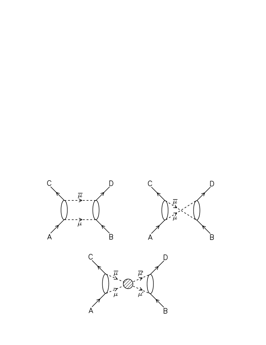
Figure 3: Two-pion and two-kaon exchange in the baryon-baryon process $A+B\to C+D$. The unshaded ellipse denotes the direct coupling of the two pseudoscalar mesons $\mu\bar{\mu}=\pi\pi,\,K\overline{K},\,\overline{K}K$ to the baryons without any correlation effects. The shaded circle in the lower diagram for the correlated exchange stands for the full off-shell amplitude of the process $\mu\bar{\mu}\to\mu^{\prime}\bar{\mu}^{\prime}$.

The Born terms for the transitions $A\overline{C}\rightarrow\pi\pi,K\overline{K}$ include contributions from baryon exchange as well as $\rho$-pole diagrams (cf. Ref. Jan95 ). The correlations between the two pseudoscalar mesons are taken into account by means of a coupled channel ($\pi\pi$, $K\bar{K}$) model Jan95 ; Loh90 generated from $s$- and $t$-channel meson exchange Born terms. This model describes the empirical $\pi\pi$ phase shifts over a large energy range from threshold up to 1.3 GeV. The amplitudes for the $A\bar{C}\rightarrow\pi\pi$, $K\bar{K}$ transitions in the pseudophysical region are then obtained by solving a covariant scattering equation with full inclusion of the $\pi\pi$ - $K\bar{K}$ correlations. The parameters of the $A\bar{C}\rightarrow\pi\pi$, $K\bar{K}$ model, which are interrelated through SU(3) symmetry, are determined by fitting to the quasiempirical $N\bar{N}\rightarrow\pi\pi$ amplitudes in the pseudophysical region, $t\leq 4m^{2}_{\pi}$ Reu96 , obtained by analytic continuation of the empirical $\pi N$ and $\pi\pi$ data.

Assuming analyticity for the amplitudes dispersion relations can be formulated for the baryon-baryon amplitudes, which connect physical amplitudes in the $s$-channel with singularities and discontinuities of these amplitudes in the pseudophysical region of the $t$-channel processes for the $J^{P}=0^{+}$ ($\sigma$) and $1^{-}$ ($\rho$) channel:

$$V^{(0^{+},1^{-})}_{A,B\to C,D}(t)\propto\int_{4m^{2}_{\pi}}^{\infty}dt^{\prime}{{\rm Im}V^{(0^{+},1^{-})}_{A,\overline{C}\to\overline{B},D}(t^{\prime})\over t^{\prime}-t},\ \ t<0.$$ (52)

Via unitarity relations the singularity structure of the baryon-baryon amplitudes for $\pi\pi$ and $K\overline{K}$ exchange are fixed by and can be written as products of the $A\overline{C}\to\pi\pi,\,K\overline{K}$ amplitudes

$${\rm Im}V^{(0^{+},1^{-})}_{A,\overline{C}\to\overline{B},D}(t^{\prime})\propto\sum_{\alpha=\pi\pi,K\overline{K}}T^{*,(0^{+},1^{-})}_{A,\overline{C}\to\alpha}\,T^{(0^{+},1^{-})}_{\overline{B},D\to\alpha}.$$ (53)

Thus, from the $A\overline{C}\rightarrow\pi\pi,\,K\overline{K}$ amplitudes the spectral functions can be calculated

$$\rho^{(0^{+},1^{-})}_{A,B\to C,D}(t^{\prime})\propto\sum_{\alpha=\pi\pi,K\overline{K}}T^{*,(0^{+},1^{-})}_{A,\bar{C}\to\alpha}\,T^{(0^{+},1^{-})}_{\bar{B},D\to\alpha}$$ (54)

which are then inserted into dispersion integrals to obtain the (on-shell) baryon-baryon interaction:

$$V^{(0^{+},1^{-})}_{A,B\to C,D}(t)\propto\int_{4m^{2}_{\pi}}^{\infty}dt^{\prime}{\rho^{(0^{+},1^{-})}_{A,B\to C,D}(t^{\prime})\over t^{\prime}-t},\ \ t<0.$$ (55)

The spectral function (54) for the ($0^{+}$) $\sigma$-channel has only one component but the one for the ($1^{-}$) $\rho$-channel consists of four linearly independent components, which reflects the more complicated spin structure of this channel Reu96 . Note that the amplitudes in Eq. (52) still contain the uncorrelated (upper diagrams in Fig. 3), as well as the correlated pieces (lower diagram). Thus, in order to obtain the contribution of the truly correlated $\pi\pi$ and $K\overline{K}$ exchange one must eliminate the former from the spectral function. This is done by calculating the spectral function generated by the Born term and subtracting it from the total spectral function:

$$\rho^{(0^{+},1^{-})}\longrightarrow\rho^{(0^{+},1^{-})}-\rho^{(0^{+},1^{-})}_{\rm Born}.$$ (56)

We should mention that the uncorrelated contributions are included too. But they are generated automatically by solving the scattering equation (1) for the interaction potential.

Finally, let us mention that the spectral functions characterize both the strength and range of the interaction. Clearly, for sharp mass exchanges the spectral function becomes a $\delta$-function at the appropriate mass.

For convenience in the concrete calculations the potential due to correlated $\pi\pi/K\overline{K}$ exchange is parametrized in terms of effective coupling strengths of (sharp mass) $\sigma$ and $\rho$ exchanges. The interaction resulting from the exchange of a $\sigma$ meson with mass $m_{\sigma}$ between two $J^{P}=1/2^{+}$ baryons $A$ and $B$ has the structure:

$$V^{\sigma}_{A,B\to A,B}(t)\ =\ g_{AA\sigma}g_{BB\sigma}{F^{2}_{\sigma}(t)\over t-m^{2}_{\sigma}},$$ (57)

where a form factor $F_{\sigma}(t)$ is applied at each vertex, taking into account the fact that the exchanged $\sigma$ meson is not on its mass shell. The correlated potential as given in Eq. (52) can now be parameterized in terms of $t$-dependent strength functions $G_{AB\to AB}(t)$, so that for the $\sigma$ case:

$$V^{(0^{+})}_{A,B\to A,B}(t)=G^{\sigma}_{AB\to AB}(t)F^{2}_{\sigma}(t){1\over t-m^{2}_{\sigma}}.$$ (58)

The effective coupling constants are then defined as

$$g_{AA\sigma}g_{BB\sigma}\quad\longrightarrow\quad G_{AB\to AB}^{\sigma}(t)={(t-m_{\sigma}^{2})\over\pi F^{2}_{\sigma}(t)}\int_{4m_{\pi}^{2}}^{\infty}{\rho^{(0^{+})}_{AB\to AB}(t^{\prime})\over t^{\prime}-t}dt^{\prime}.$$ (59)

In the concrete application one varies $m_{\sigma}^{2}$ in order to achieve that $G_{AB\to AB}^{\sigma}(t)\approx G_{AB\to AB}^{\sigma}$, i.e. that $G_{AB\to AB}^{\sigma}$ is indeed practically a constant. The form factor is parameterized by

$$F_{\sigma}(t)={\Lambda^{2}_{\sigma}\over\Lambda^{2}_{\sigma}-t}\ ,$$ (60)

with a cut–off mass $\Lambda_{\sigma}$ assumed to be the same for both vertices. This form guarantees that the on-shell behaviour of the potential (which is fully determined by the dispersion integral) is not modified strongly as long as the energy is not too high.

Similar relations can be also derived for the correlated exchange in the isovector-vector channel Reu96 , which in this case will involve vector as well as tensor coupling pieces.

4.2 Other ingredients of the Jülich meson-exchange hyperon-nucleon model

Besides the correlated $\pi\pi$ and $K\bar{K}$ exchange the new $YN$ model of the Jülich group takes into account exchange diagrams involving the well-established lowest lying pseudoscalar and vector meson SU(3) octets. Following the philosophy of the original Jülich $YN$ potential Hol89 the coupling constants in the pseudoscalar sector are fixed by strict SU(6) symmetry. In any case, this is also required for being consistent with the model of correlated $\pi\pi$ and $K\overline{K}$ exchange. The cut–off masses of the form factors (cf. discussion at the beginning of Sect. 4) belonging to the $NN$ vertices are taken over from the full Bonn $NN$ potential. The cut–off masses at the strange vertices are considered as open parameters though, in practice, their values are kept as close as possible to those found for the $NN$ vertices.

In addition there are some other new ingredients in the present $YN$ model as compared to the earlier Jülich models Hol89 ; Reu94 . First of all, we now take into account contributions from (scalar-isovector) $a_{0}(980)$ exchange. The $a_{0}$ meson is present in the original Bonn $NN$ potential MHE , and for consistency should also be included in the $YN$ model. Secondly, we consider the exchange of a strange scalar meson, the $\kappa$, with mass $\sim 1000$ MeV. Let us emphasize, however, that like in case of the $\sigma$ meson these particles are not viewed as being members of a scalar meson SU(3) multiplet, but rather as representations of strong meson-meson correlations in the scalar–isovector ($\pi\eta$–$K\overline{K}$) Jan95 and scalar–isospin-1/2 ($\pi K$) channels Loh90 , respectively. In principle, their contributions can also be evaluated along the lines of Ref. Reu96 , however, for simplicity in the present model they are effectively parameterized by one-boson-exchange diagrams with the appropriate quantum numbers assuming the coupling constants to be free parameters. Furthermore, the new model contains the exchange of an $\omega^{\prime}$ with a mass of $m_{\omega^{\prime}}$ = 1120 MeV considered to be an effective parametrization of short-range contributions from correlated $\pi-\rho$ exchange Jan96 in the vector-isoscalar sector. Its inclusion allows to keep the coupling constants of the genuine $\omega$(782) meson to the baryons in line with their SU(3) values, cf. the discussion in Ref. Hai05 . In the spirit of the EFT approach, we have also considered a version of the $YN$ potential in Hai05 where the $\kappa$ exchange was substituted by a local contact interaction.

Thus we have the following scenario: The long- and intermediate-range part of the new meson-exchange $YN$ interaction model is completely determined by SU(6) constraints (for the pseudoscalar and, in general, also for the vector mesons) and by correlated $\pi\pi$ and $K\overline{K}$ exchange. The short-range part is viewed as being due to correlated meson-meson exchanges but in practice is parametrized phenomenologically in terms of one-boson-exchange contributions in specific spin-isospin channels. In particular, no SU(3) relations are imposed on the short-range part. This assumption is based on our observation that the contributions in the $\rho$ exchange channel as they result from correlated $\pi\pi$ and $K\bar{K}$ no longer fulfill strict SU(3) relations Reu96 , but it also acknowledges the fact that at present there is no general agreement about who are the actual members of the lowest-lying scalar meson SU(3) multiplet, as already mentioned above. A graphical representation of all meson-exchange contributions that are included in the new $YN$ model is given in Fig. 4.

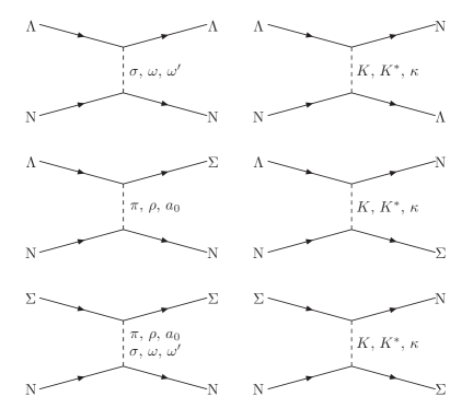
Figure 4: Contributions to the meson-exchange $YN$ model Hai05 in the $\Lambda N$ and $\Sigma N$ channels and in the $\Lambda N\to\Sigma N$ transition. Note that only $\pi$, $K$, $\omega$, and $K^{*}$ exchange are considered as being due to genuine SU(3) mesons. The other contributions are either fixed from correlated $\pi\pi$ and $K\overline{K}$ exchange ($\sigma$, $\rho$) or are viewed as an effective parametrization of meson-meson correlations ($a_{0}$, $\kappa$, $\omega$’) in the corresponding spin-isospin channels.

5 Results and discussion

In Fig. 5 we confront the results obtained from our $YN$ interactions with the $\Lambda p$, $\Sigma^{+}p$, $\Sigma^{-}p$, $\Sigma^{-}p\to\Sigma^{0}n$, and $\Sigma^{-}p\to\Lambda n$ data used in the fitting procedure. Here the solid curves correspond to the Jülich ’04 meson-exchange model and the shaded band represents the results of the chiral EFT for the considered cut–off region. For reasons of comparison we also include the results of one of the meson-exchange models (NSC97f) of the Nijmegen group (dashed line) Rij99 . A detailed comparison between the experimental scattering data considered and the values found in the fitting procedure for the EFT interaction (for $\Lambda=600$ MeV) is given in Table 3.

Table 3: Comparison between the 35 experimental $YN$ data and the results for the EFT interaction for the cut–off $\Lambda=600$ MeV. Momenta are in units of MeV and cross sections in mb. The achieved $\chi^{2}$ is given for each reaction channel separately.

$\Lambda p\rightarrow\Lambda p\;\;$ $\chi^{2}=7.5$			$\Lambda p\rightarrow\Lambda p\;\;$ $\chi^{2}=4.9$			$\Sigma^{-}p\rightarrow\Lambda n\;\;$ $\chi^{2}=5.5$
$p_{{\rm lab}}^{\Lambda}$	$\sigma_{{\rm exp}}$Sec68	$\sigma_{{\rm the}}$	$p_{{\rm lab}}^{\Lambda}$	$\sigma_{{\rm exp}}$Ale68	$\sigma_{{\rm the}}$	$p_{{\rm lab}}^{\Sigma^{-}}$	$\sigma_{{\rm exp}}$Eng66	$\sigma_{{\rm the}}$
135	209$\pm$58	170.0	145	180$\pm$22	161.6	110	174$\pm$47	244.2
165	177$\pm$38	145.4	185	130$\pm$17	130.4	120	178$\pm$39	210.0
195	153$\pm$27	123.5	210	118$\pm$16	113.7	130	140$\pm$28	183.0
225	111$\pm$18	104.7	230	101$\pm$12	101.9	140	164$\pm$25	161.4
255	87 $\pm$13	89.1	250	83 $\pm$13	91.5	150	147$\pm$19	143.9
300	46 $\pm$11	70.6	290	57 $\pm$9	74.3	160	124$\pm$14	129.5
$\Sigma^{+}p\rightarrow\Sigma^{+}p\;\;$ $\chi^{2}=0.6$			$\Sigma^{-}p\rightarrow\Sigma^{-}p\;\;$ $\chi^{2}=2.4$			$\Sigma^{-}p\rightarrow\Sigma^{0}n\;\;$ $\chi^{2}=7.0$
$p_{{\rm lab}}^{\Sigma^{+}}$	$\sigma_{{\rm exp}}$Eis71	$\sigma_{{\rm the}}$	$p_{{\rm lab}}^{\Sigma^{-}}$	$\sigma_{{\rm exp}}$Eis71	$\sigma_{{\rm the}}$	$p_{{\rm lab}}^{\Sigma^{-}}$	$\sigma_{{\rm exp}}$Eng66	$\sigma_{{\rm the}}$
145	123$\pm$62	96.7	142.5	152$\pm$38	143.4	110	396$\pm$91	200.0
155	104$\pm$30	93.0	147.5	146$\pm$30	137.5	120	159$\pm$43	177.4
165	92 $\pm$18	89.6	152.5	142$\pm$25	131.9	130	157$\pm$34	159.3
175	81 $\pm$12	86.7	157.5	164$\pm$32	126.8	140	125$\pm$25	144.7
			162.5	138$\pm$19	122.1	150	111$\pm$19	132.7
			167.5	113$\pm$16	117.6	160	115$\pm$16	122.7
$r^{{\rm exp}}_{R}=0.468\pm 0.010$			$r^{{\rm the}}_{R}=0.475$			$\chi^{2}=0.5$

The differential cross sections are calculated in the usual way using the partial wave amplitudes, for details we refer to Hol89 ; Fra80 . The total cross sections are found by simply integrating the differential cross sections, except for the $\Sigma^{+}p\to\Sigma^{+}p$ and $\Sigma^{-}p\rightarrow\Sigma^{-}p$ channels. For those channels the experimental total cross sections were obtained via Eis71

$$\sigma = \frac{2}{\cos\theta_{{\rm max}}-\cos\theta_{{\rm min}}}\int_{\cos\theta_{{\rm min}}}^{\cos\theta_{{\rm max}}}\frac{d\sigma(\theta)}{d\cos\theta}d\cos\theta\ ,$$ (61)

for various values of $\cos\theta_{{\rm min}}$ and $\cos\theta_{{\rm max}}$. Following Rij99 , we use $\cos\theta_{{\rm min}}=-0.5$ and $\cos\theta_{{\rm max}}=0.5$ in our calculations for the $\Sigma^{+}p\rightarrow\Sigma^{+}p$ and $\Sigma^{-}p\rightarrow\Sigma^{-}p$ cross sections, in order to stay as close as possible to the experimental procedure.

A good description of the low-energy $YN$ scattering data has been obtained with the discussed meson-exchange models but also within the EFT approach in the considered cut–off region, as is documented in Tables 2 and 3 and Figs. 5 and 6.

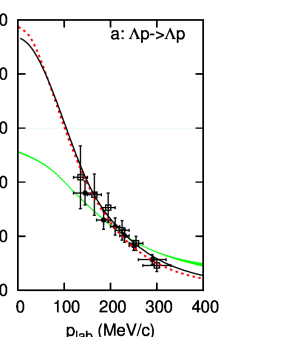
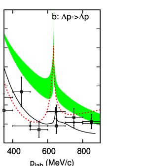
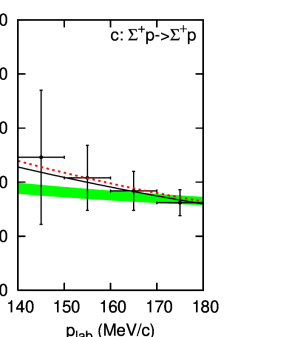
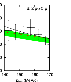
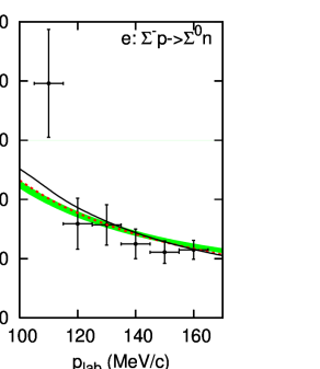
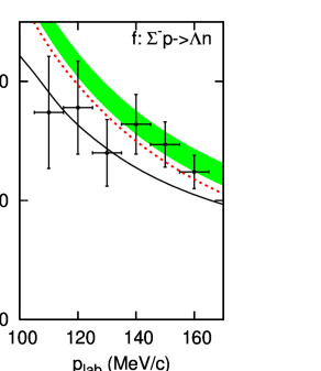
Figure 5: ”Total” cross section $\sigma$ (as defined in Eq. (61)) as a function of $p_{{\rm lab}}$. The experimental cross sections in (a) are taken from Refs. Sec68 (open squares) and  Ale68 (filled circles), in (b) from Refs. Kad71 (filled circles) and Hau77 (open squares) , in (c),(d) from Eis71 and in (e),(f) from Eng66 . The shaded band is the chiral EFT result for $\Lambda=550,...,700$ MeV Pol06 , the solid curve is the Jülich ’04 model Hai05 , and the dashed curve is the Nijmegen NSC97f potential Rij99 .

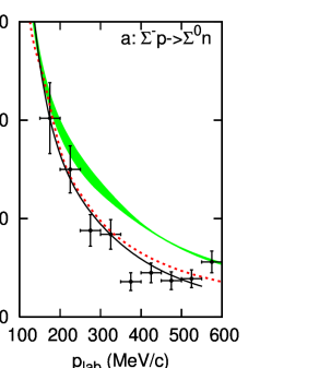
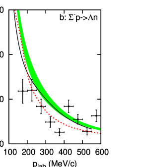
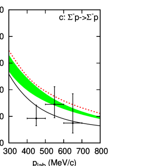
Figure 6: As in Fig. 5, but now the experimental cross sections in (a),(b) are taken from Refs. Ste70 and in (c) from Kon00 .

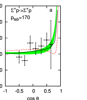
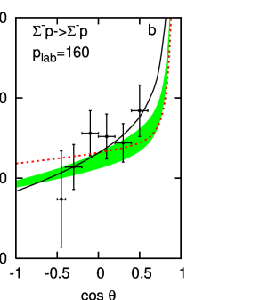
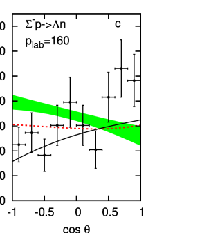
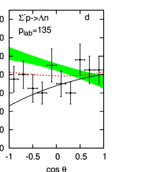
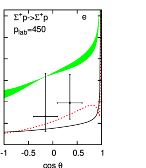
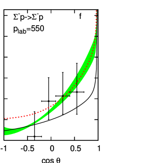
Figure 7: Differential cross section $d\sigma/d\cos\theta$ as a function of $\cos\theta$, where $\theta$ is the c.m. scattering angle, at various values of $p_{{\rm lab}}$ (MeV/c). The experimental differential cross sections in (a),(b) are taken from Eis71 , in (c),(d) from Eng66 , in (e) from Ahn99 and in (f) from Kon00 . Same description of curves as in Fig. 5.

Note that in the low-energy regime the cross sections are mainly given by the $S$-wave contribution, except for for the $\Lambda N\rightarrow\Sigma N$ cross section where the ${}^{3}D_{1}(\Lambda N)\leftrightarrow{}^{3}S_{1}(\Sigma N)$ transition provides the main contribution. Still all partial waves with total angular momentum $J\leq 2$ were included in the computation of the observables. The $\Lambda p$ cross sections show a clear cusp at the $\Sigma^{+}n$ threshold, see Fig. 5b. This cusp is very pronounced for the EFT interaction, peaking at 60 mb, but also in case of the Nijmegen NSC97f model. It is hard to see this effect in the experimental data, since it occurs over a very narrow energy range. In case of the EFT interaction the predicted $\Lambda p$ cross section at higher energies is too large (cf. Fig. 5b), which is related to the problem that some LO phase shifts are too large at higher energies. Note that this is also the case for the $NN$ interaction Epe00a . In a NLO calculation this problem will probably vanish. The differential cross sections at low energies, which have not been taken into account in the fitting procedure, are predicted well, see Fig. 7. The results of the meson-exchange models and of the chiral EFT are also in good agreement with data for total cross sections at higher energy Ste70 ; Kon00 which were likewise not included in the fitting procedure, as can be seen in Fig. 6.

The $\Lambda p$ and $\Sigma^{+}p$ scattering lengths and effective ranges are listed in Table 4 together with the corresponding hypertriton binding energies (preliminary results of $YNN$ Faddeev calculations from Nog06 ).

Table 4: The $YN$ singlet and triplet scattering lengths and effective ranges (in fm) and the hypertriton binding energy, $E_{B}$ (in MeV). The binding energies for the hypertriton (last row) Nog06 are calculated using the Idaho-N3LO $NN$ potential Entem:2003ft . The experimental value of the hypertriton binding energy is $-2.354(50)$ MeV Gibson:1995an . We notice that the deuteron binding energy is $-2.224$ MeV.

	EFT ’06				Jülich ’04	NSC97f Rij99
$\Lambda$ [MeV]	550	600	650	700
$a^{\Lambda p}_{s}$	$-1.90$	$-1.91$	$-1.91$	$-1.91$	$-2.56$	$-2.51$
$r^{\Lambda p}_{s}$	$1.44$	$1.40$	$1.36$	$1.35$	$2.75$	$3.03$
$a^{\Lambda p}_{t}$	$-1.22$	$-1.23$	$-1.23$	$-1.23$	$-1.66$	$-1.75$
$r^{\Lambda p}_{t}$	$2.05$	$2.13$	$2.20$	$2.27$	$2.93$	$3.32$
$a^{\Sigma^{+}p}_{s}$	$-2.24$	$-2.32$	$-2.36$	$-2.29$	$-4.71$	$-4.35$
$r^{\Sigma^{+}p}_{s}$	$3.74$	$3.60$	$3.53$	$3.63$	$3.31$	$3.14$
$a^{\Sigma^{+}p}_{t}$	$0.70$	$0.65$	$0.60$	$0.56$	$0.29$	$-0.25$
$r^{\Sigma^{+}p}_{t}$	$-2.14$	$-2.78$	$-3.55$	$-4.36$	$-11.54$	$-25.35$
$(^{3}_{\Lambda}\rm H)$ $E_{B}$	$-2.35$	$-2.34$	$-2.34$	$-2.36$	$-2.27$	$-2.30$

The magnitudes of the $\Lambda p$ singlet and triplet scattering lengths obtained within chiral EFT are smaller than the corresponding values of the Jülich ’04 and Nijmegen NSC97f models (last two columns), which is also reflected in the small $\Lambda p$ cross section near threshold, see Fig. 5a. But despite of this significant difference the EFT interaction yields a correctly bound hypertriton too, see last row in Table 4. The singlet $\Sigma^{+}p$ scattering length predicted by chiral EFT is about half as large as the values found for the meson-exchange $YN$ potentials. Like in the latter models and other $YN$ interactions, the value of the triplet $\Sigma^{+}p$ scattering length obtained by chiral EFT is fairly small. Contrary to NSC97f, but as in the Jülich ’04 $YN$ model, there is repulsion in this partial wave.

Some $S$- and $D$-wave phase shifts for $\Lambda p$ and $\Sigma^{+}p$ are shown in Fig. 8. As mentioned before, the limited accuracy of the $YN$ scattering data does not allow for a unique phase shift analysis. This explains why the chiral EFT phase shifts are quite different from the phase shifts of the new meson-exchange $YN$ interaction of the Jülich group but also from all models presented in Ref. Rij99 . Indeed, the predictions of the various meson-exchange models also differ between each other in most of the partial waves. In both the $\Lambda p$ and $\Sigma^{+}p$ ${}^{1}S_{0}$ and ${}^{3}S_{1}$ partial waves, the LO chiral EFT phase shifts are much larger at higher energies than the phases of the meson-exchange models. But this is not surprising. First we want to remind the reader that the empirical data $YN$ considered in the fitting procedure are at lower energies. Second, also for the $NN$ interaction in leading order these partial waves were much larger than the Nijmegen phase shift analysis, see Epe00a . It is expected that this problem for the $YN$ interaction can be solved by the derivative contact terms in a NLO calculation, just like in the $NN$ case. It is interesting to see that the ${}^{3}S_{1}$ $\Sigma^{+}p$ phase shift is repulsive in chiral EFT as well as in the new Jülich meson-exchange model, but attractive in the Nijmegen NSC97f model. This has consequences for the $\Sigma^{+}p$ differential cross section because, depending on the sign, the interference of the hadronic amplitude with the Coulomb amplitude differs, cf. Fig. 7. Unfortunately, the limited accuracy of the available $\Sigma^{+}p$ data does not allow to discriminate between these two scenarios.

Results for $P$-wave phase shifts can be found in Refs. Rij99 ; Hai05 ; Pol06 . Here we just want to remark that in case of LO chiral EFT the $P$-waves are the result of pseudoscalar meson exchange alone, since we only have contact terms in the $S$-waves in that order. Also, contrary to conventional meson-exchange models, in LO chiral EFT there are no spin singlet to spin triplet transitions, because of the potential form in Eqs. (25) and (49). Although the ${}^{3}D_{1}$ $\Lambda p$ phase shift near the $\Sigma N$ threshold rises quickly for our $YN$ interactions, cf. Fig. 8, it does not go through 90 degrees in both cases – unlike the Nijmegen model NSC97f Rij99 . The opening of the $\Sigma N$ channel is also clearly seen in the ${}^{3}S_{1}$ $\Lambda p$ partial wave for all considered interactions, but again there are significant differences in the concrete behavior.

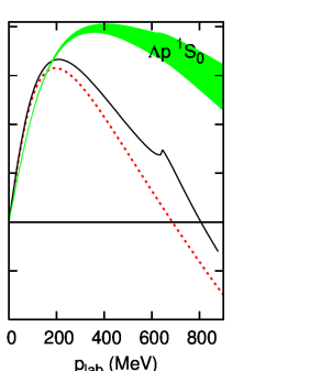
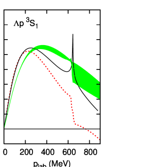
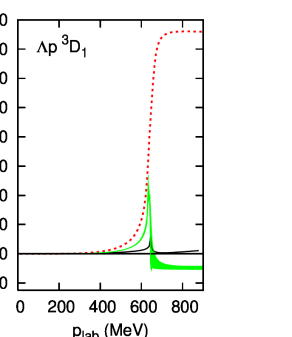
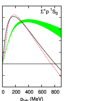
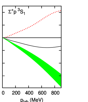
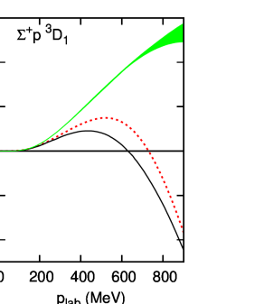
Figure 8: The $\Lambda p$ and $\Sigma^{+}p$ $S$-wave and ${}^{3}D_{1}$ phase shifts $\delta$ as a function of $p_{{\rm lab}}$. Since the phases of the Jülich ’04 model are calculated in the isospin basis, its $\Sigma N$ threshold does not exactly coincide with the others. Same description of curves as in Fig. 5.

Very recently the chiral EFT model has been employed in Faddeev-type investigations of the four-body systems ${}^{4}_{\Lambda}$H and ${}^{4}_{\Lambda}$He Nog06a . The binding energies of these hypernuclei are especially interesting predictions. It is has been very difficult in the past to describe their charge symmetry breaking (CSB) and the splitting of the $0^{+}$ ground and $1^{+}$ excited state at the same time Nogga:2001ef . In Table 5, we show the differences of the binding energies of the core nucleus and the hypernucleus, the $\Lambda$ separation energies, since these are only mildly dependent on the $NN$ interaction model used for the calculations Nogga:2001ef . We compare the $\Lambda$ separation energies based on chiral EFT and the two considered meson-exchange $YN$ interactions to the experimental numbers. It is seen that the separation energies for the excited states are somewhat dependent on the cut–off value chosen. Certainly, contributions from higher order will be sizable for these observables. However, within these uncertainties, the results agree remarkably well with the experimental separation energies, which is somewhat less the case for the meson-exchange potentials. The CSB of the separation energies is not well described by all of the interactions. The Nijmegen model NSC97f includes explicit CSB in the potential, which induces a sizable but too small effect on the separation energies. It will be interesting to study this observable in NLO of the chiral interaction, where first explicitly CSB terms contribute.

Table 5: $\Lambda$ separation energies of the $0^{+}$ ($E_{sep}(0^{+})$) and $1^{+}$ ($E_{sep}(1^{+})$) states and their difference $\Delta E_{sep}$ for ${}^{4}_{\Lambda}$H and the difference of the separation energies for the mirror hypernuclei ${}^{4}_{\Lambda}$He and ${}^{4}_{\Lambda}$H (CSB-$0^{+}$ and CSB-$1^{+}$). Results for the chiral EFT $YN$ interaction for various cut–offs $\Lambda$ are compared to predictions for the Jülich ’04 and Nijmegen NSC97f meson-exchange models and the experimental values Gibson:1995an .

	EFT ’06				Jülich ’04	NSC97f	Expt.
$\Lambda$ [MeV]	500	550	650	700
$E_{sep}(0^{+})$ [MeV]	2.63	2.46	2.36	2.38	1.87	1.60	2.04
$E_{sep}(1^{+})$ [MeV]	1.85	1.51	1.23	1.04	2.34	0.54	1.00
$\Delta E_{sep}$ [MeV]	0.78	0.95	1.13	1.34	-0.48	0.99	1.04
CSB-$0^{+}$ [MeV]	0.01	0.02	0.02	0.03	-0.01	0.10	0.35
CSB-$1^{+}$ [MeV]	-0.01	-0.01	-0.01	-0.01	—	-0.01	0.24

6 Summary and outlook

In this review we presented results based on two different approaches to the $YN$ interaction, namely on the traditional meson-exchange picture and on chiral effective field theory.

As far as meson-exchange models of the $YN$ interaction are concerned we focussed on the recent model of the Jülich group, whose main new feature is that the contributions both in the scalar-isoscalar ($\sigma$) and the vector-isovector ($\rho$) channels are constrained by a microscopic model of correlated $\pi\pi$ and $K\overline{K}$ exchange. Besides those contributions from correlated $\pi\pi$ and $K\overline{K}$ exchange this model incorporates also the standard one-boson exchanges of the lowest pseudoscalar and vector meson multiplets with coupling constants fixed by SU(6) symmetry relations. Thus, the long- and intermediate-range part of this $YN$ interaction model is completely determined – either by SU(6) constraints or by correlated $\pi\pi$ and $K\overline{K}$ exchange.

The $YN$ interaction derived within chiral EFT is based on a modified Weinberg power counting, analogous to the $NN$ force in Epe05 . The symmetries of QCD are explicitly incorporated. Also here it is assumed that the interactions in the various $YN$ channels are related via ${\rm SU(3)}_{f}$ symmetry. However, since we have done our study in leading order, in which the $NN$ interaction can not be described well, we do not connect the present $YN$ interaction with the $NN$ sector, but focus on the $YN$ system only.

To be specific, the leading-order potential consists of two pieces: firstly, the longer-ranged one-pseudoscalar-meson exchanges, related via ${\rm SU(3)}_{f}$ symmetry in the well-known way and secondly, the shorter ranged four-baryon contact term without derivatives. The latter contains five independent low-energy constants that need to be determined from the empirical data. We fixed those five free parameters by fitting to 35 low-energy $YN$ scattering data. The reaction amplitude is obtained by solving a regularized Lippmann-Schwinger equation for the chiral EFT interaction. The regularization is done by multiplying the strong potential with an exponential regulator function where we used a cut–off in the range between $550$ and $700$ MeV.

The meson-exchange picture has been already applied successfully to the $YN$ system in the past by many authors. Thus, it is not surprising that a good reproduction of the data could be achieved within this approach. But it is rather reassuring to see that also chiral effective field theory works remarkably well for the $YN$ interaction, in particular since we have, so far, restricted ourselves to lowest order only. Indeed, we could obtain a rather good description of the empirical data, as is reflected in the total $\chi^{2}$ which is the range between $28.3$ and $34.6$ for a cut–off in the range between $550$ and $700$ MeV. In addition low-energy differential cross sections and higher energy cross sections, that were not included in the fitting procedure, were predicted quite well.

In a first application to few-baryon systems involving strangeness we found that the chiral EFT yields a correctly bound hypertriton Nog06 . We did not explicitly include the hypertriton binding energy in the fitting procedure, but we have fixed the relative strength of the $\Lambda N$ singlet and triplet $S$-waves in such a way that a bound hypertriton could be obtained. It is interesting to note that a $\Lambda p$ singlet scattering length of $-1.9$ fm leads to the correct binding energy. Meson-exchange $YN$ models that yield comparable results for the hypertriton binding energy predict here singlet scattering lengths that are typically in the order of $-2.5$ fm.

In conclusion, our results strongly suggest that the chiral effective field theory scheme, applied in Ref. Epe05 to the $NN$ interaction, also works well for the $YN$ interaction. In the future it will be interesting to study the convergence of the chiral EFT for the $YN$ interaction by doing NLO and NNLO calculations. In particular a combined $NN$ and $YN$ study in chiral EFT, starting with a NLO calculation, needs to be performed. Also an SU(3) extension to the hyperon-hyperon ($YY$) sector is of interest. In this case only one additional low-energy constant arises within the EFT approach in LO. This constant could be fixed by available data on the reaction $\Xi^{-}p\to\Lambda\Lambda$ Ahn06 , say, and then predictions can be made for all reaction channels in the strangeness -2 sector. In particular, one would then be able to obtain an estimate for the $\Lambda\Lambda$ interaction, whose strength is rather crucial for the existence of doubly strange hypernuclei. With regard to the interactions presented in this review it will be interesting to see their performance when employed in further calculations of strange few-baryon systems as well as in hypernuclei. For example, preliminary results for the four-body hypernuclei ${}^{4}_{\Lambda}{\rm H}$ and ${}^{4}_{\Lambda}{\rm He}$ show that the chiral EFT predicts reasonable $\Lambda$ separation energies for ${}^{4}_{\Lambda}{\rm H}$, though the charge dependence of the $\Lambda$ separation energies is not reproduced (as expected at lowest order).

References

- (1) R. Machleidt, K. Holinde, and C. Elster, Phys. Rep. 149, 1 (1987).
- (2) R. Machleidt and I. Slaus, J. Phys. G27, R69 (2001).
- (3) P. M. M. Maessen, T. A. Rijken, and J. J. de Swart, Phys. Rev. C 40, 2226 (1989).
- (4) B. Holzenkamp, K. Holinde, and J. Speth, Nucl. Phys. A500, 485 (1989).
- (5) A. Reuber, K. Holinde, and J. Speth, Nucl. Phys. A570, 543 (1994).
- (6) K. Tominaga et al., Nucl. Phys. A642, 483 (1998).
- (7) T. A. Rijken, V. G. J. Stoks, and Y. Yamamoto, Phys. Rev. C 59, 21 (1999).
- (8) K. Tominaga and T. Ueda, Nucl. Phys. A693, 731 (2001).
- (9) J. Haidenbauer and U.-G. Meißner, Phys. Rev. C 72, 044005 (2005).
- (10) T. A. Rijken and Y. Yamamoto, Phys. Rev. C 73, 044008 (2006).
- (11) E. Klempt, F. Bradamante, A. Martin, and J.-M. Richard, Phys. Rept. 368, 119 (2002).
- (12) P. F. Bedaque and U. van Kolck, Annu. Rev. Nucl. Part. Sci. 52, 339 (2002).
- (13) D. Kaplan, nucl-th/0510023 .
- (14) E. Epelbaum, Prog. Nucl. Part. Phys. 57, 654 (2006).
- (15) E. Epelbaum, W. Glöckle, and U.-G. Meißner, Nucl. Phys. A747, 362 (2005).
- (16) D. R. Entem and R. Machleidt, Phys. Rev. C68, 041001 (2003).
- (17) S. Weinberg, Phys. Lett. B251, 288 (1990).
- (18) S. Weinberg, Nucl. Phys. B363, 3 (1991).
- (19) E. Epelbaoum, W. Glöckle, and U.-G. Meißner, Nucl. Phys. A637, 107 (1998).
- (20) M. J. Savage and M. B. Wise, Phys. Rev. D 53, 349 (1996).
- (21) H. W. Hammer, Nucl. Phys. A705, 173 (2002).
- (22) C. L. Korpa, A. E. L. Dieperink, and R. G. E. Timmermans, Phys. Rev. C 65, 015208 (2001).
- (23) D. B. Kaplan, M. J. Savage, and M. B. Wise, Nucl. Phys. B534, 329 (1998).
- (24) S. R. Beane, P. F. Bedaque, A. Parreño, and M. J. Savage, Nucl. Phys. A747, 55 (2005).
- (25) S. R. Beane et al., hep-lat/0612026 .
- (26) H. Polinder, J. Haidenbauer, and U.-G. Meißner, Nucl. Phys. A779, 244 (2006).
- (27) C. M. Vincent and S. C. Phatak, Phys. Rev. C 10, 391 (1974).
- (28) M. Walzl, U.-G. Meißner, and E. Epelbaum, Nucl. Phys. A693, 663 (2001).
- (29) J. D. Bjorken and S. D. Drell, Relativistic Quantum Fields, McGraw-Hill Inc., New York, 1965. We follow the conventions of this reference.
- (30) T.-P. Cheng and L.-F. Li, Gauge theory of elementary particle physics, Oxford University Press, Oxford, 1984.
- (31) T. A. Rijken, R. A. M. Klomp, and J. J. de Swart, in A Gift of Prophecy, Essays in Celebration of the Life of Robert Eugene Marshak, edited by E. C. G. Sudarshan, World Scientific, Singapore, 1995.
- (32) J. J. de Swart, Rev. Mod. Phys. 35, 916 (1963).
- (33) C. B. Dover and H. Feshbach, Ann. Phys. 198, 321 (1990).
- (34) E. Epelbaum, W. Glöckle, and U.-G. Meißner, Nucl. Phys. A671, 295 (2000).
- (35) U.-G. Meißner, Rep. Prog. Phys. 56, 903 (1993).
- (36) E. Epelbaum et al., Eur. Phys. J. A 15, 543 (2002).
- (37) E. Epelbaum, W. Glöckle, and U.-G. Meißner, Eur. Phys. J. A 19, 401 (2004).
- (38) B. Sechi-Zorn, B. Kehoe, J. Twitty, and R. A. Burnstein, Phys. Rev. 175, 1735 (1968).
- (39) G. Alexander et al., Phys. Rev. 173, 1452 (1968).
- (40) F. Eisele, H. Filthuth, W. Fölisch, V. Hepp, and G. Zech, Phys. Lett 37B, 204 (1971).
- (41) R. Engelmann, H. Filthuth, V. Hepp, and E. Kluge, Phys. Lett. 21, 587 (1966).
- (42) J. J. de Swart and C. Dullemond, Ann. Phys. 19, 485 (1962).
- (43) M. M. Nagels, T. A. Rijken, and J. J. de Swart, Phys. Rev. D 15, 2547 (1977).
- (44) E. Klempt, hep-ph/0404270 .
- (45) Y. Kalashnikova, A. E. Kudryavtsev, A. V. Nefediev, J. Haidenbauer, and C. Hanhart, Phys. Rev. C73, 045203 (2006).
- (46) A. Reuber, K. Holinde, H.-C. Kim, and J. Speth, Nucl. Phys. A608, 243 (1996).
- (47) G. Janssen, B. Pierce, K. Holinde, and J. Speth, Phys. Rev. D 52, 2690 (1995).
- (48) D. Lohse, J. Durso, K. Holinde, and J. Speth, Nucl. Phys. A516, 513 (1990).
- (49) G. Janssen, K. Holinde, and J. Speth, Phys. Rev. C 54, 2218 (1996).
- (50) P. La France and P. Winternitz, J. Physique 41, 1391 (1980).
- (51) J. A. Kadyk, G. Alexander, J. H. Chan, P. Gaposchkin, and G. H. Trilling, Nucl. Phys. B27, 13 (1971).
- (52) J. M. Hauptman, J. A. Kadyk, and G. H. Trilling, Nucl. Phys. B125, 29 (1977).
- (53) D. Stephen, PhD thesis, University of Massachusetts, 1975, unpublished.
- (54) Y. Kondo et al., Nucl. Phys. A676, 371 (2000).
- (55) J. K. Ahn et al., Nucl. Phys. A648, 263 (1999).
- (56) A. Nogga, J. Haidenbauer, H. Polinder, and U.-G. Meißner, in preparation.
- (57) B. F. Gibson and E. V. Hungerford, Phys. Rept. 257, 349 (1995).
- (58) A. Nogga, nucl-th/0611081 .
- (59) A. Nogga, H. Kamada, and W. Glöckle, Phys. Rev. Lett. 88, 172501 (2002).
- (60) J. Ahn et al., Phys. Lett. B 633, 214 (2006).