A Global Model of $\beta^{-}$-Decay Half-Lives Using Neural Networks

Abstract

Statistical modeling of nuclear data using artificial neural networks (ANNs) and, more recently, support vector machines (SVMs), is providing novel approaches to systematics that are complementary to phenomenological and semi-microscopic theories. We present a global model of $\beta^{-}$-decay halflives of the class of nuclei that decay 100% by $\beta^{-}$ mode in their ground states. A fully-connected multilayered feed forward network has been trained using the Levenberg-Marquardt algorithm, Bayesian regularization, and cross-validation. The halflife estimates generated by the model are discussed and compared with the available experimental data, with previous results obtained with neural networks, and with estimates coming from traditional global nuclear models. Predictions of the new neural-network model are given for nuclei far from stability, with particular attention to those involved in r-process nucleosynthesis. This study demonstrates that in the framework of the $\beta^{-}$-decay problem considered here, global models based on ANNs can at least match the predictive performance of the best conventional global models rooted in nuclear theory. Accordingly, such statistical models can provide a valuable tool for further mapping of the nuclidic chart.

1 Introduction

Currently, there is an urgent need for reliable estimates of $\beta^{-}$-decay halflives of nuclei far from stability. This need is driven both by the experimental programs of existing and future radioactive ion-beam facilities and by ongoing efforts toward understanding supernova explosions and the processes of nucleosynthesis in stars, notably the r-process [1]. Such estimates are also needed to provide guidance for nuclear structure theory itself, as totally new areas of the nuclear landscape are opened for exploration. Several models for determining $\beta^{-}$ halflives have been proposed and applied during the last few decades. These include the more phenomenological models based on Gross Theory as well as models (in various versions) that employ the Quasiparticle Random-Phase Approximation (QRPA), along with some approaches based on shell-model calculations. The latest version of Gross Theory, known as the Semi-Gross Theory (SGT), incorporates shell effects of the parent nucleus [2]. Extensive proton-neutron ($pn$) QRPA calculations have been carried out by two groups. The latest version of the models developed by the first group (Klapdor and coworkers) takes account of $pp$ and $pn$ forces and includes a schematic interaction for the first-forbidden (ff) $\beta$ decay (NBSC+pnQRPA) [3]. The latest version of the models developed by the second group (Möller and coworkers) combines the $pn$QRPA model with the statistical Gross Theory of ff decay (pnQRPA+ffGT) [4]. There is also a model of $\beta^{-}$-decay halflives in which the ground state of the parent nucleus is described by the extended Thomas-Fermi plus Strutinsky integral method and the continuum QRPA (CQRPA) [5]. Recently, a relativistic $pn$QRPA model has been applied in the treatment of neutron-rich nuclei in the $N=50$ and 82 regions [6]. Although there is continuous improvement, the predictive power of these conventional models is rather limited for $\beta^{-}$-decay halflives of nuclei that are mainly far from the stability, with deviations from experiment of at least an order of magnitude. This being the case, statistical modeling based on artificial neural networks (ANNs) and other adaptive techniques of statistical inference presents an interesting and potentially effective alternative for global modeling of $\beta$-decay lifetimes, as it does for other problems in nuclear systematics. Neural-network models have already been developed for other nuclear properties, including atomic masses, neutron separation energies, ground-state spins and parities, and branching probabilities in different decay channels, as well as $\beta^{-}$ halflives [7]. Very recently, global statistical models of some of these properties have also been developed based on Support Vector Machines (SVMs) [8]. In the present work [9], which continues a previous effort in statistical modeling of nuclear half-life systematics [7,10,11], we present a new global model for the halflives of nuclear ground states that decay 100% by the $\beta^{-}$ mode. The model is a feedforward artificial neural network (FF-ANN) which has been constructed by means of a more sophisticated technology than applied previously. The predictive power of this model is as good or better than that of the existing models created within nuclear theory. The methodology adopted is outlined in Sect. 2. Some results from the model are reported and evaluated in Sect. 3, which is followed in Sect. 4 by a brief summary and prospectus.

2 Methodology

After a large number of computer experiments on networks constructed with various choices of architectures, training and initialization algorithms, forms of activation function, and scaling of variables, we have arrived at an ANN model that is effective not only in approximating the observed $\beta^{-}$ decay half-life systematics, but also generalizes quite well to unknown regions of the nuclidic chart. This model is a fully connected feedforward (FF) multilayer network model with architecture symbolized by $[3-5-5-5-5-1|116]$. The activation functions of the neuron-like units are given by a hyperbolic-tangent sigmoid function in the intermediate (hidden) layers and a saturated linear function in the output layer. The three input units encode the atomic number $Z$, the neutron number $N$, and the corresponding pairing constant $\delta$ defined as

$$\delta=\left\{{\begin{array}[]{*{20}c}{+1,}\\ {0,}\\ {-1,}\\ \end{array}\begin{array}[]{*{20}c}{\begin{array}[]{*{20}c}{\rm for}&{\rm even-even}&{\rm nuclei}\,,\\ \end{array}}\\ {\begin{array}[]{*{20}c}{\rm for}&{\rm odd-mass}&{\rm nuclei}\,,\\ \end{array}}\\ {\begin{array}[]{*{20}c}{\rm for}&{\rm odd-odd}&{\rm nuclei}\,.\\ \end{array}}\\ \end{array}}\right.$$ (10)

When $Z$, $N$, and $\delta$ are fed into the input interface, the network performs its calculation and the single output unit decodes the network’s response – i.e., its estimate for $\log T_{1/2}$, the base-10 log of the $\beta^{-}$ halflife of nuclide $(Z,N)$. The four hidden layers, each containing five neuronal units, transfer information from input to output, processing it through weighted connections (or biases), in this case 116 in number. The central idea of neural-network modeling is that such parameters can be adjusted through a proper training algorithm to produce good overall performance on a training (or learning) set and good generalization on test nuclei absent from the training set. We have adopted the Levenberg-Marquardt optimization algorithm to train the network, while implementing a combination of two well-established techniques for improving generalization, namely, Bayesian regularization and cross-validation [12]. The Nguyen-Widrow method [12] was chosen for initialization of the network. The experimental data for our modeling of $\beta^{-}$ halflives have been taken from the Nubase2003 evaluation of nuclear and decay properties due to G. Audi et al. [13]. Considering only those cases in which the parent ground state decays 100% by the $\beta^{-}$ channel, we form a preliminary set made up of 905 nuclides. The halflives of nuclides in this set range from $0.15\times 10^{-2}\,{\rm s}$ for ³⁵Na to $2.43\times 10^{23}\,{\rm s}$ for ¹¹³Cd. We have worked mostly with a restricted set of 843 nuclides, formed by elimination of those nuclei having halflife greater than $10^{6}\,{\rm s}$. With the exclusion of these long-lived examples, one is dealing with a smaller but more homogeneous collection of nuclides that facilitates the training of the network. From the 843 nuclides (overall set) (sorted according to the value of the half-life), 503 ($\sim$ 60%) have been uniformly selected to serve as training examples (learning set); of those left over, 167 ($\sim$ 20%) have been also uniformly chosen to validate the learning procedure (validation set); and the remaining 168 nuclides ($\sim$ 20%) are reserved to test the accuracy of prediction (prediction set). This partitioning of the data was adopted to ensure that the distribution over halflives in the whole set is faithfully reflected in the learning, validation, and prediction sets.

The performance of the statistical model so designed and constructed is evaluated with the aid of two commonly used statistical metrics, namely the root-mean-square error (RMSE) and the mean-absolute-square error (MAE):

$${\rm RMSE}=\left[{\frac{1}{N_{\alpha}}\sum\limits_{k}{\left({y_{k}-\hat{y}_{k}}\right)^{2}}}\right]^{1/2}\,,\qquad{\rm MAE}=\frac{1}{N_{\alpha}}\sum\limits_{k}{\left|{y_{k}-\hat{y}_{k}}\right|}\,.$$ (11)

Here, ${\hat{y}_{k}}$ is the experimentally measured value of the base-10 logarithm of the halflife of nuclide $k$, and $y_{k}$ is the estimate of this quantity (the “calculated value”) produced by the network model. The sums in definitions (11) run over the $N_{\alpha}$ nuclides in the learning, validation, or prediction set, as appropriate. Smaller values of these metrics indicate higher accuracy. In the training procedure adopted, the RMSE was taken as the cost function, or objective function, to be minimized by adjustment of the weight parameters of the network.

In the literature on global modeling of $\beta^{-}$ lifetimes, several different figures of merit have been used to analyze model performance. The collaboration led by Klapdor [3] employs the average deviation defined by

$$\langle x\rangle_{K}=\frac{1}{N_{\alpha}}\sum\limits_{i}{x_{i}}\,,$$ (12)

where $x_{i}$ is given by $T_{{1/2},{({\rm exp})}}^{(i)}/T_{{1/2},{({\rm calc})}}^{(i)}$ if $T_{{1/2},{({\rm exp})}}^{(i)}\geq T_{{1/2}^{({\rm calc})}}^{(i)}$, the ratio otherwise being inverted, along with the corresponding standard deviation

$$\sigma_{K}=\left[{\frac{1}{N_{\alpha}}\sum\limits_{i}{\left({x_{i}-\langle x\rangle_{K}}\right)^{2}}}\right]^{{1\mathord{\left/{\vphantom{12}}\right.\kern-1.2pt}2}}.$$ (13)

(Again, the sums run over the appropriate set of nuclides.) Following Klapdor and coworkers, a more incisive analysis is achieved by determining the percentage $m$ of nuclides having measured ground-state halflife $T_{{1\mathord{\left/{\vphantom{1{2,{\rm exp}}}}\right.\kern-1.2pt}{2,{\rm exp}}}}$ within a prescribed range (e.g., not greater than $10^{6}$ $s$, 60 $s$, or 1 $s$), for which the calculated halflife is within a prescribed tolerance factor $f$ (in particular 2, 5, or 10) of the experimental value. Möller et al. [4] have used a measure $M_{r}$ similar to $\langle x\rangle_{K}$, but defined in terms of $\log_{10}T_{1/2}$ rather than $T_{1/2}$. Thus, they analyzed model performance in terms of the mean value of $r_{k}=y_{k}/{\hat{y}_{k}}$ and its associated standard deviation, given respectively by

$$M_{r}=\frac{1}{N_{\alpha}}\sum_{k}r_{k}\quad{\rm and}\quad\sigma_{r}=\left[\frac{1}{N_{\alpha}}\sum_{k}(r_{k}-M_{r})^{2}\right]^{1/2}\,.$$ (14)

Somewhat more useful are the mean deviation (range) and mean fluctuation (range), defined respectively as

$$M^{(10)}=10^{M_{r}}\quad{\rm and}\quad\sigma_{M^{(0)}}=10^{\sigma_{r}}\,.$$ (15)

For a closer analysis, these indices may again be calculated within prescribed halflife ranges.

3 Results

Table 1 presents the RMSE and the MAE of our global model on the indicated data sets. Also included for comparison are some results from an antecedent ANN model [10]. The improvement represented by the current model is apparent.

Table 1: Root-mean-square errors (RMSE) and mean-absolute errors (MAE) (Eqs. (11)) for learning, validation, and prediction subsets and the full data set (overall set), for current and previous FF-ANN models of $\beta^{-}$ lifetime systematics [10].

Current FF-ANN Model			Previous FF-ANN Model [10]
$[3-5-5-5-5-1|116]$			$[16-10-1|181]$
Data Set	RMSE	MAE	Data Set	RMSE
Learning	0.53	0.38	Learning	1.08
Validation	0.60	0.41	-	-
Prediction	0.65	0.46	Prediction	1.82
Overall	0.57	0.40	-	-

Next, adopting the performance metric of Möller and collaborators (Eqs. (14)-(15)), our model is compared with two global models based on the proton-neutron Quasiparticle Random-Phase Approximation ($pn$QRPA), namely the NBSC+$pn$QRPA model of Homma et al. [3] and the FRDM+$pn$QRPA model of Möller et al. [14]. Table 2 contains the results for $M^{(10)}$ and $\sigma_{M^{(10)}}$, according to the even-even, odd-odd, and odd-mass-number character of nuclides, excluding halflives greater than 1000 s. As seen in the table, the $pn$QRPA models tend to overestimate halflives for odd-odd nuclei (except for the shorter-lived nuclides in the FRDM+$pn$QRPA case). The FRDM+$pn$QRPA model also overestimates halflives for even-even nuclei. Our model also tends to overestimate the halflives of even-even nuclei, but to a substantially smaller degree. This shortcoming of the ANN model is partly due to the more limited abundance of these nuclei.

Table 2: Values of the performance measures $M^{(10)}$ and $\sigma_{M^{(10)}}$ (Eqs. (14)-(15)) for the current FF-ANN model (overall and prediction sets) and for the NBSC+pnQRPA [3] and FRDM+pnQRPA [14] models.

$\bf T_{{1\mathord{\left/{\vphantom{1{2,{\bf exp}}}}\right.\kern-1.2pt}{2,{\rm exp}}}}$		Overall Set			Prediction Set
(sec)	char.	$n$	$M^{(10)}$	$\sigma_{M^{(10)}}$	$n$	$M^{(10)}$	$\sigma_{M^{(10)}}$
$f<1$	o-o	76	1.04	2.53	11	0.86	1.98
	odd	125	1.16	2.25	32	1.05	2.40
	e-e	51	1.87	2.45	7	2.36	3.26
$f<10$	o-o	121	1.11	2.96	20	0.86	3.76
	odd	187	1.10	2.31	42	0.92	2.61
	e-e	87	1.65	2.56	17	1.80	2.58
$f<100$	o-o	158	1.08	3.06	28	0.76	3.20
	odd	261	1.08	2.45	57	0.97	2.91
	e-e	110	1.58	2.31	21	1.58	2.98
$f<1000$	o-o	191	1.12	3.06	35	0.78	3.13
	odd	329	1.07	2.73	68	0.84	3.07
	e-e	133	1.63	2.60	28	1.49	3.04
$\bf T_{{1\mathord{\left/{\vphantom{1{2,{\bf exp}}}}\right.\kern-1.2pt}{2,{\rm exp}}}}$		NBSC+pnQRPA [3]			FRDM+pnQRPA [14]
(sec)	char.	$n$	$M^{(10)}$	$\sigma_{M^{(10)}}$	$n$	$M^{(10)}$	$\sigma_{M^{(10)}}$
$f<1$	o-o	28	1.75	4.96	29	0.59	2.91
	odd	31	0.60	2.24	35	0.59	2.64
	e-e	10	1.15	2.36	10	3.84	3.08
$f<10$	o-o	66	1.89	4.60	59	0.76	8.83
	odd	81	0.92	3.84	85	0.78	4.81
	e-e	34	1.01	2.93	34	2.50	4.13
$f<100$	o-o	85	3.15	10.5	88	2.33	49.2
	odd	127	1.07	4.29	133	1.11	9.45
	e-e	52	1.13	3.58	54	2.61	4.75
$f<1000$	o-o	93	3.02	10.2	115	3.50	72.0
	odd	157	1.10	5.55	194	2.77	71.5
	e-e	63	1.39	6.10	71	6.86	58.5

The efficacy of our latest FF-ANN model has also been evaluated in terms of the metrics introduced by Klapdor and coworkers (Eqs. (12)-(13)). Table 3 includes our results as well as those of the NBSC+$pn$QRPA model [3]. Comparing the two models, especially the values for the percentage $m$, it is evident that the neural-network model is superior in estimating the $\beta^{-}$ lifetimes, both for the totality of the data and for the prediction set. The ANN model has the ability to reproduce approximately 90% of experimentally known halflives shorter than $10^{6}\,{\rm s}$ within a factor of 10 and about 50% within a factor of 2. That $m$ is reduced only slightly in going from the overall set to the prediction set is indicative of good generalization. However, the way in which the three subsets (for training, validation, and testing) were chosen dictates that the prediction involved in generating the results of Table 3 is primarily a matter of interpolation rather than extrapolation.

Table 3: Values of the performances measures $\langle x\rangle_{K}$ and $\sigma_{K}$ (Eqs. (12)-(13)) for our FF-ANN model (overall and prediction sets) and for the NBSC+$pn$QRPA model [3]. Also given are results for the percentage $m$ of nuclides having measured halflife within the prescribed range, for which the halflife given by the model lies within a tolerance factor $f$ of the experimental value.

	$\bf T_{{1\mathord{\left/{\vphantom{1{2,{\bf exp}}}}\right.\kern-1.2pt}{2,{\rm exp}}}}$	Overall Set			Prediction Set			NBSC+pnQRPA [3]
$f$	(sec)	m(%)	$\langle x\rangle_{K}$	$\sigma_{K}$	m(%)	$\langle x\rangle_{K}$	$\sigma_{K}$	m(%)	$\langle x\rangle_{K}$	$\sigma_{K}$
$f<10$	$<10^{6}$	92.0	2.46	1.72	90.5	2.69	1.85	76.7	3.00	-
	$<60$	96.5	2.21	1.52	96.1	2.48	1.64	87.2	2.81	-
	$f<1$	97.6	2.10	1.39	98.0	2.24	1.30	95.7	2.64	-
$f<5$	$<10^{6}$	82.8	1.99	0.95	79.2	2.10	0.97	-	-	-
	$<60$	90.2	1.88	0.84	87.3	2.05	0.91	-	-	-
	$f<1$	93.7	1.88	0.80	94.0	2.04	0.89	-	-	-
$f<2$	$<10^{6}$	53.5	1.41	0.27	49.4	1.48	0.28	33.8	1.43	-
	$<60$	60.6	1.41	0.27	53.9	1.48	0.27	42.0	1.41	-
	$f<1$	61.9	1.41	0.26	60.0	1.50	0.27	50.7	1.43	-

Thus, the capability of the ANN model in interpolation having been established, we must now assess its potential for extrapolation, or “extrapability.” In this aspect of model behavior, we expect a similar level of performance as seen in Table 3, for the early extrapolation regions close in $Z$ and $N$ to the learning and validation sets. Fig. 2 shows estimated halflives for nuclides in the Ni isotopic chain along with available experimental data, while Fig. 2 presents analogous results for the $N=82$ isotonic chain. For comparison, the plots include corresponding estimates from the hybrid $pn$QRPA+ffGT model [4], as well as results of some calculations by Pfeiffer, Kratz, and Möller [15] (GT*) based on the early Gross Theory (GT) of Takahashi et al. [16] but with updated mass values [17, 18]. It is interesting to compare the various predictions for the halflife of the doubly magic r-process ⁷⁸Ni nucleus ($N=50$, $Z=28$) with the value that was recently measured by Hosmer et al. [19] (Fig. 2). Our result lies within the error bar.

There is no firm and quantitative guideline by which the behavior of the different calculations can be judged, either theoretical or statistical, in the ranges where there are no experimental data. Nevertheless, one does expect, from the observed behavior of known nuclei, that the more neutron-rich an exotic isotope is, the shorter its halflife will be. This projected downward tendency under increasing $N$ is seen in all of the models considered. One does anticipate more drastic dependence of the halflife on the even/odd character of two neighboring isotopes. This sawtooth behavior is present in our ANN model, but it is probably somewhat exaggerated. The same behavior appears, if to a lesser degree, in continuum-Quasiparticle-RPA (CQRPA) approaches [5] and in other calculations [4, 16].

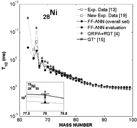
Figure 1: Halflives $T_{1/2}$ for $\beta^{-}$ decay of nuclides in the isotopic chain of ₂₈Ni. Included are experimental data and results of various models (see legend). The new measurement for the doubly magic r-process nuclide ${}^{78}_{28}$Ni is included (see legend).

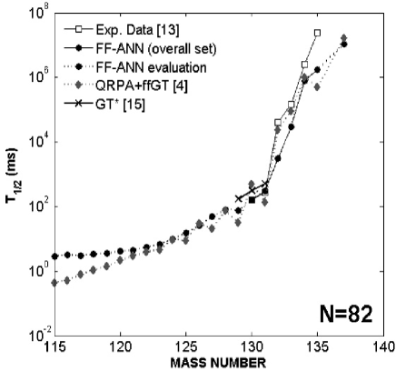
Figure 2: As in Fig. 2, but for the isotonic chain of $N=82$.

4 Conclusion and Prospects

The results presented here demonstrate that global statistical models based on Artificial Neural Networks have strong potential for successful exploitation of the accelerated acquisition of nuclear data and could provide a valuable tool in exploring the nature of $\beta^{-}$ halflives outside the stable valley. Accordingly, we plan further studies of the systematics of $\beta$ decay, employing still more advanced ANN models that embody new state-of-the-art optimization algorithms and more sophisticated training strategies, with the object of continued enhancement of the predictive power of these learning machines.

5 Acknowledgments

This research has been supported in part by the U. S. National Science Foundation under Grant No. PHY-0140316 and by the University of Athens under Grant No. 70/4/3309.

References

- [1] Opportunities in Nuclear Science: “A Long Range Plan in the Next Decade”(DOE/NSF, 2002); “Long Range Plan 2004” (NUPECC, 2004).
- [2] H. Nakata, T. Tachibana, M. Yamada, Nucl. Phys. A625, 521 (1997).
- [3] H. Homma et al., Phys. Rev. C 54, 2972 (1996).
- [4] P. Moller, B. Pfeiffer, K.-L. Kratz, Phys. Rev. C 67, 055802 (2003).
- [5] I. N. Borzov, S. Goriely, Phys. Rev. C 62 (2000) 035501.
- [6] T. Niksič et al., Phys. Rev. C 71 (2005) 014308.
- [7] J. W. Clark, in Scientific Applications of Neural Nets, J. W. Clark, T. Lindenau, M. L. Ristig, eds. (Springer, Berlin, 1999), p. 1; K. A. Gernoth, ibid., p. 139.
- [8] H. Li, J. W. Clark, E. Mavrommatis, S. Athanassopoulos, K. A. Gernoth, in Condensed Matter Theories, Vol. 20, J. W. Clark, R. M. Panoff, H. Li, eds. (Nova Science Publishers, N.Y. 2006) p. 505, nucl-th/0506080; J. W. Clark, H. Li, in Recent Progress in Many-Body Theories, Vol. 8, S. Hernandez and H. Cataldo, eds. (World Scientific, Singapore, 2006), nucl-th/0603037.
- [9] N. Costiris, E. Mavrommatis, K. A. Gernoth, J. W. Clark, to be published.
- [10] E. Mavrommatis, A. Dakos, K. A. Gernoth, J. W. Clark, Condensed Matter Theories, Vol. 13, J. da Providencia, F. B. Malik, eds. (Nova Sciences Publishers, Commack, NY, 1998), p. 423.
- [11] J. W. Clark, E. Mavrommatis, S. Athanassopoulos, A. Dakos, K. A. Gernoth”, Fission Dynamics of Atomic Clusters and Nuclei, D. M. Brink, F. F. Karpechine, F. B. Malik, and J. da Providencia, eds. (World Scientific, Singapore), pp. 76-85. [nucl-th/0109081]
- [12] H. Demuth, M. Beale, Guide Version 4 (The Mathworks Inc., 2000).
- [13] G. Audi, O. Bersillon, J. Blachot, A. H. Wapstra, Nucl. Phys. A729, 3 (2003).
- [14] P. Moller, J. R. Nix, K.-L. Kratz, At. Data Nucl. Data Tables 66, 131 (1997).
- [15] B. Pfeiffer, K.-L. Kratz, P. Moller, Institut für Kernchemie Internal Report (2003).
- [16] K. Takahashi, M. Yamada, T. Kondoh, At. Data Nucl. Data Tables 12, 101 (1973).
- [17] P. Moller, J. R. Nix, W. D. Myers, W. J. Swiatecki, At. Data Nucl. Data Tables 59, 185 (1995).
- [18] G. Audi, A. H. Wapstra, Nucl. Phys. A595, 409 (1995).
- [19] P. T. Hosmer et al., Phys. Rev. Lett. 94, 112501 (2005)