The Pion Cloud of the Nucleon: Facts and popular Fantasies

Abstract

I discuss the concept of the pion cloud surrounding the nucleon and other hadrons - and its limitations.

1 Introduction

Long before QCD, meson theory was invented to describe the nuclear forces Yuk . It was quickly realized that pion-nucleon scattering data require a large coupling constant. As a further consequence of this strong coupling, many virtual mesons – Yukawas pions – were expected to be associated with the nucleon. This was the birth of the pion cloud, the main topic of this contribution. Heisenberg and Wentzel developed a consistent approach to the strong coupling limit, treating the mesons as classical fields and the finite nucleon size providing an UV cutoff. For an early calculation of that period, see e.g. Ref. FHK . Many of these ideas have survived until today, but now we know that low-energy QCD is governed by the spontaneous breakdown of its chiral symmetry (for the light quarks) with the pion taking over a special role as a (Pseudo-)Goldstone boson. In this talk, I will be concerned with the pionic contribution to the nucleon (hadron) structure, loosely called the “pion cloud”. There is no doubt that is an important part of nucleon structure, but the main questions to be addressed are: i) is it possible to uniquely and unambiguously define the contribution of the “pion cloud” to any given observable? and ii) how could such a contribution be quantified? There is lots of folklore about this issue, my goal is to be more precise and show that while this concept provides a nice intuitive picture, it can hardly be made quantitative without resorting to uncontrolled models. But let us go step by step. The first question can best be addressed in the framework of chiral perturbation theory (CHPT) (for a recent review, see BMrev ). To be precise, consider a single nucleon. In baryon CHPT a nucleon typically emits a pion, this energetically forbidden $\pi$N intermediate state lives for a short while and then the pion is reabsorbed by the nucleon, in accordance with the uncertainty principle. This mechanism is responsible for the venerable old idea of the “pion cloud” of the nucleon, which in CHPT can be put on the firm ground of field theoretical principles. This will be discussed in more detail in the next section. As will be shown, such loop contributions are in general not scale-independent and thus can not provide the required model-independent definition. I will then analyze the low-energy structure of the nucleons’ electromagnetic form factors and show which constraints are set by fundamental principles (like unitarity and chiral symmetry) on their pionic contribution. This will then allow for an – albeit model-dependent – extraction of the longest range contribution to these fundamental nucleon structure quantities. Throughout this talk, I eschew models.

2 Chiral loops as a representation of the pion cloud

Beyond tree level, any observable calculated in CHPT receives contributions from tree and loop graphs. Naively, these loop diagrams qualify as the natural candidate for a precise definition of the “pion cloud” of any given hadron. The loop graphs not only generate the imaginary parts of the pertinent observables but are also – in most cases – divergent, requiring regularization and renormalization. In CHPT, one usually chooses a mass–independent regularization scheme to avoid power divergences (there are, however, instances where other regulators are more appropriate or physically intuitive. For a beautiful discussion of this and related issues, see e.g. Refs. Georgi:1994qn ; Espriu:1993if ). The method of choice in CHPT is dimensional regularization (DR), which introduces the scale $\lambda$. Varying this scale has no influence on any observable $O$ (renormalization group invariance),

$$\frac{d}{d\lambda}\,O(\lambda)=0~{},$$ (1)

but this also means that it makes little sense to assign a physical meaning to the separate contributions from the contact terms and the loops. Physics, however, dictates the range of scales appropriate for the process under consideration — describing the pion vector radius (at one loop) by chiral loops alone would necessitate a scale of about 1/2 TeV (as stressed long ago by Leutwyler). In this case, the coupling of the $\rho$–meson generates the strength of the corresponding one-loop counterterm that gives most of the pion radius — more on this below. The most intriguing aspects of chiral loops are the so-called chiral logarithms (chiral logs). In the chiral limit, the pion cloud becomes long-ranged and there is no more Yukawa factor $\sim\exp(-M_{\pi}r)$ to cut it off. This generates terms like $\log M^{2}_{\pi},1/M_{\pi},\ldots$, that is contributions that are non–analytic in the quark masses. Such statements can be applied to all hadrons that are surrounded by a cloud of pions which by virtue of their small masses can move away very far from the object that generates them. Stated differently, in QCD the approach to the chiral limit is non–analytic in the quark masses and the low–energy structure of QCD can therefore not be analyzed in terms of a simple Taylor expansion. The exchange of the massless Goldstone bosons generates poles and cuts starting at zero momentum transfer, such that the Taylor series expansion in powers of the momenta fails. This is a general phenomenon of theories that contain massless particles – the Coulomb scattering amplitude due to photon exchange is proportional to $e^{2}/t$, with $t=(p^{\prime}-p)^{2}$ the momentum transfer squared between the two charged particles. Let me return to the discussion of the chiral loops. As stated before, most loops are divergent. In DR, all one–loop divergences are simple poles in $1/(d-4)$, where $d$ is the number of space-time dimensions. Consequently, these divergences can be absorbed in the pertinent low-energy constants (LECs) that accompany the corresponding local operators at that order in harmony with the underlying symmetries. For a given LEC $L_{i}$ this amounts to $L_{i}\to L_{i}^{\rm ren}+\beta_{i}\,{\rm L}(\lambda)~{},$ where ${\rm L}\sim 1/(d-4)$ and $\beta_{i}$ is the corresponding $\beta$–function. The renormalized and finite $L_{i}^{\rm ren}$ must be determined by a fit to data (or calculated eventually using lattice QCD). Having determined the values of the LECs from experiment, one is faced with the issue of trying to understand these numbers. Not surprisingly, the higher mass states of QCD leave their imprint in the LECs. Consider again the $\rho$-meson contribution to the vector radius of the pion. Expanding the $\rho$-propagator in powers of $t/M_{\rho}^{2}$, its first term is a contact term of dimension four, with the corresponding finite LEC $L_{9}$ given by $L_{9}=F_{\pi}^{2}/2M_{\rho}^{2}\simeq 7.2\cdot 10^{-3}$, close to the empirical value $L_{9}=6.9\cdot 10^{-3}$ at $\lambda=M_{\rho}$. This so–called resonance saturation (pioneered in Refs.Ecker:1988te ; Ecker:1989yg ; Donoghue:1988ed ) holds more generally for most LECs at one loop and is frequently used in two–loops calculations to estimate the ${\cal O}(p^{6})$ LECs (for a recent study on this issue, see Kampf:2006bn ). Let us now discuss the the “pion cloud” of the nucleon in the context of these considerations. Consider as an example the isovector Dirac radius of the proton Bernard:2003rp (for precise definitions, see the next section). The first loop contributions appear at third order in the chiral expansion, leading to

$$\langle r^{2}\rangle_{1}^{V}=\left(0.61-\left(0.47\,{\rm GeV}^{2}\right)\,\tilde{d}(\lambda)+0.47\log\frac{\lambda}{1\,{\rm GeV}}\right)~{}{\rm fm}^{2}~{},$$ (2)

where $\tilde{d}(\lambda)$ is a dimension three pion–nucleon LEC that parameterizes the “nucleon core” contribution. Compared to the empirical value $(r_{1}^{v})^{2}=0.585$ fm² MMD we note that several combinations of $(\lambda,\tilde{d}(\lambda))$ pairs can reproduce the empirical result, e.g.

$$\left(1~{}\rm{GeV},+0.06~{}\rm{GeV}^{-2}\right),\left(0.943~{}\rm{GeV},\rm{0.00~{}GeV}^{-2}\right),\left(0.6~{}\rm{GeV},-0.46~{}\rm{GeV}^{-2}\right)\,.$$ (3)

An important observation to make is that even the sign of the “core” contribution to the radius can change within a reasonable range typically used for the scale $\lambda$. Physical intuition would tell us that the value for the coupling $\tilde{d}$ should be negative such that the nucleon core gives a positive contribution to the isovector Dirac radius, but field theory tells us that for (quite reasonable) regularization scales above $\lambda=943$ MeV this need not be the case. In essence, only the sum of the core and the cloud contribution constitutes a meaningful quantity that should be discussed. This observation holds for any observable - not just for the isovector Dirac radius discussed here.

3 Nucleon electromagnetic form factors: Basic definitions

To analyze the pion cloud contribution to the nucleons’ electromagnetic form factors in more detail, we must collect some basic definitions. These form factors are defined by the nucleon matrix element of the quark electromagnetic current,

$$\langle N(p^{\prime})|\bar{q}\gamma^{\mu}{\hat{Q}}q|N(p)\rangle=\bar{u}(p^{\prime})\left[\gamma^{\mu}\,F_{1}(q^{2})+\frac{i}{2m}\sigma^{\mu\nu}(p^{\prime}-p)_{\nu}\,F_{2}(q^{2})\right]u(p)~{},$$ (4)

with $q^{2}=(p^{\prime}-p)^{2}=t$ the invariant momentum transfer squared, ${\hat{Q}}$ the quark charge matrix, and $m$ the nucleon mass. $F_{1}(q^{2})$ and $F_{2}(q^{2})$ are the Dirac and the Pauli form factors, respectively. Following the conventions of MMD , we decompose the form factors into isoscalar ($S$) and isovector ($V$) components,

$$F_{i}(q^{2})=F_{i}^{S}(q^{2})+\tau_{3}\,F_{i}^{V}(q^{2})~{},\quad i=1,2\,,$$ (5)

subject to the normalization $F_{1}^{S}(0)=F_{1}^{V}(0)=1/2\,,$ $F_{2}^{S,V}(0)=(\kappa_{p}\pm\kappa_{n})/{2}~{},$ with $\kappa_{p}\,(\kappa_{n})=1.793\,(-1.913)$ the anomalous magnetic moment of the proton (neutron). We will also use the Sachs form factors,

$$G_{E}^{I}(q^{2})=F_{1}^{I}(q^{2})+\frac{q^{2}}{4m^{2}}F_{2}^{I}(q^{2})~{},\quad G_{M}^{I}(q^{2})=F_{1}^{I}(q^{2})+F_{2}^{I}(q^{2})~{},\quad I=S,V~{}.$$ (6)

These are commonly referred to as the electric and the magnetic nucleon form factors. The slope of the form factors at $q^{2}=0$ can be expressed in terms of a nucleon radius

$$\langle r^{2}\rangle_{i}^{I}=\frac{6}{F_{i}^{I}(0)}\left.\frac{dF_{i}^{I}(q^{2})}{dq^{2}}\right|_{q^{2}=0}\,,\quad i=1,2\,,\quad I=S,V\,,$$ (7)

and analogously for the Sachs form factors. The analysis of the nucleon electromagnetic form factors proceeds most directly through the spectral representation given by

$$F_{i}^{I}(q^{2})=\frac{1}{\pi}\,\int_{{(\mu_{0}^{I})}^{2}}^{\infty}\frac{\sigma_{i}^{I}(\mu^{2})\,d\mu^{2}}{\mu^{2}-q^{2}}~{},\quad i=1,2~{},\quad I=S,V~{},$$ (8)

in terms of the real spectral functions $\sigma_{i}^{I}(\mu^{2})={\rm Im}\,F_{i}^{I}(\mu^{2})$. The corresponding thresholds are given by $\mu_{0}^{S}=3M_{\pi}$, $\mu_{0}^{V}=2M_{\pi}$, with $M_{\pi}$ the charged pion mass. Since the isovector spectral function is non–vanishing for smaller momentum transfer (starting at the two–pion cut) than the isoscalar one (starting at the three–pion cut), the isovector spectral functions plays a more important role in the question of the pionic contribution to the nucleon structure. More precisely, let us consider the nucleon form factors in the space-like region. In the Breit–frame (where no energy is transferred), any form factor $F$ can be written as the Fourier–transform of a coordinate space density,

$$F({\bf q}^{2})=\int d^{3}{\bf r}\,{\rm e}^{i{\bf q}\cdot{\bf r}}\,\rho(r)~{},$$ (9)

with ${\bf q}$ the three–momentum transfer. In particular, comparison with Eq. (8) allows us to express the density $\rho(r)$ in terms of the spectral function

$$\rho(r)=\frac{1}{4\pi^{2}}\,\int_{\mu_{0}^{2}}^{\infty}d\mu^{2}\,\sigma(\mu^{2})\,\frac{{\rm e}^{-\mu r}}{r}~{}.$$ (10)

Note that for the electric and the magnetic Sachs form factor, $\rho(r)$ is nothing but the charge and the magnetization density, respectively. For the Dirac and Pauli form factors, Eq. (10) should be considered as a formal definition. This equation expresses the density as a linear combination of Yukawa distributions, each of mass $\mu$. The lightest mass hadron is the pion, and from Eq. (10) it is evident that pions are responsible for the long–range part of the electromagnetic structure of the nucleon. This contribution is commonly called the “pion cloud” of the nucleon and in fact this long–range low–$q^{2}$ contribution to the nucleon form factors can be directly derived from unitarity or be calculated on the basis of chiral perturbation theory, as discussed next.

4 Spectral functions and their low-energy constraints

The spectral functions defined in Eq. (8) are the central quantities in the dispersion-theoretical approach. They can in principle be constructed from experimental data. In practice, this program can only be carried out for the lightest two-particle intermediate states. Higher mass contributions are usually parameterized in terms of vector meson poles. For the discussion of the pion cloud, only the lightest mass (longest range) contributions to the spectral functions are of relevance. These will be discussed next.

Isovector case: Let us now evaluate the two–pion contribution in a model–independent way and draw some conclusions on the spatial extent of the pion cloud from that (see the next section). As pointed out long ago FF and further elaborated on in Ref. HP , unitarity allows us to determine the isovector spectral functions from threshold up to masses of about 1 GeV in terms of the pion charge form factor $F_{\pi}(t)$ and the P–wave $\pi\pi\bar{N}N$ partial waves, see Fig. 1. We use here the form

$${\rm Im}~{}G_{E}^{V}(t)=\frac{q_{t}^{3}}{m\sqrt{t}}\,\left|F_{\pi}(t)\right|^{2}\,J_{+}(t)~{},~{}~{}~{}{\rm Im}~{}G_{M}^{V}(t)=\frac{q_{t}^{3}}{\sqrt{2t}}\,\left|F_{\pi}(t)\right|^{2}\,J_{-}(t)~{},$$ (11)

where $q_{t}=\sqrt{t/4-M_{\pi}^{2}}$. The functions $J_{\pm}(t)$ are related to the $t$–channel P–wave $\pi$N partial waves $f_{\pm}^{1}(t)$ via $f_{\pm}^{1}(t)=F_{\pi}(t)\,J_{\pm}(t)$ in the conventional isospin decomposition, with the tabulated values of the $J_{\pm}(t)$ from LB . For the pion charge form factor $F_{\pi}$ we use the latest experimental data from CMD-2 CMD2 , KLOE KLOE , and SND SND .

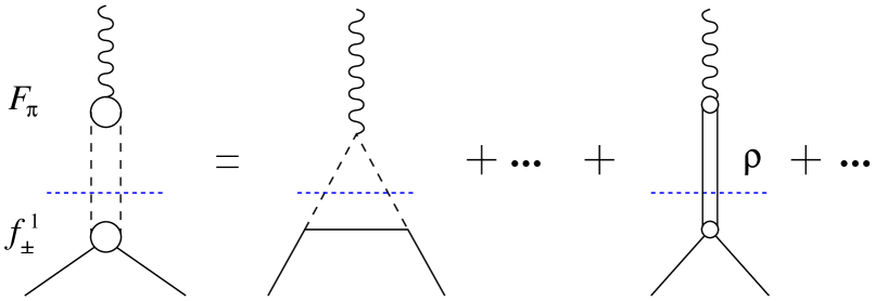
Figure 1: Two–pion contribution to the isovector nucleon form factors. On the left side, the exact representation based on unitarity is shown, whereas the triangle diagram on the right side leads to the strong enhancement of the isovector spectral functions close to threshold. Also shown is the dominant $\rho$–meson contribution. The solid, dashed, wiggly and double lines represent nucleons, pions, photons and the $\rho$, respectively.

We stress that the representation of Eq. (11) gives the exact isovector spectral functions for $4M_{\pi}^{2}\leq t\leq 16M_{\pi}^{2}$ but in practice holds up to $t\simeq 50M_{\pi}^{2}$. It has two distinct features. First, as already pointed out in FF , it contains the important contribution of the $\rho$–meson (see Fig. 1) with its peak at $t\simeq 30M_{\pi}^{2}$. Second, on the left shoulder of the $\rho$, the isovector spectral functions display a very pronounced enhancement close to the two–pion threshold, as shown in Fig. 2 (taken from Ref. BHM2pi ).

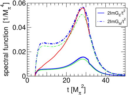
Figure 2: The two-pion spectral function using the new high statistics data for the pion form factor CMD2 ; KLOE ; SND . The spectral functions weighted by $1/t^{2}$ are shown for $G_{E}$ (solid line) and $G_{M}$ (dash-dotted line). The previous results by Höhler et al. LB (without $\rho$-$\omega$ mixing) are shown for comparison by the gray/green lines. The red solid line indicates the $\rho$-meson contribution to Im $G_{M}$ with a width $\Gamma_{\rho}=150\,$MeV.

This is due to the logarithmic singularity on the second Riemann sheet located at $t_{c}=4M_{\pi}^{2}-M_{\pi}^{4}/m^{2}=3.98M_{\pi}^{2}$, very close to the threshold. This pole comes from the projection of the nucleon Born graphs, or in modern language, from the triangle diagram also depicted in Fig. 1 (middle graph). If one were to neglect this important unitarity correction, one would severely underestimate the nucleon isovector radii HP2 . In fact, precisely the same effect is obtained at leading one–loop accuracy in chiral perturbation theory, as discussed first in GSS ; BKMrev . This topic was further elaborated on in the framework of heavy baryon CHPT BKMspec ; Norbert and in a covariant calculation based on infrared regularization KM (see also Schindler:2005ke ). It is important to note that there is a strict one-to-one correspondence between this unitarity correction and the field-theoretically defined one-pion loop – contrary to what is claimed in de Jager’s contribution to this workshop deJager:2006nt . Stated differently, the most important two–pion contribution to the nucleon form factors can be determined by using either unitarity or CHPT (in the latter case, of course, the $\rho$ contribution is not included). Clearly, this is an important input into the spectral functions used in the on-going dispersive analysis of the nucleon form factors by the Bonn-Mainz group MMD ; HMD ; HM ; BHMff (see also the work by Dubnicka and collaborators as reviewed in Ref. Adamuscin:2005aq ).

Isoscalar case: In the isoscalar electromagnetic channel, it was believed (but not proven) that the pertinent spectral functions rise smoothly from the three–pion threshold to the $\omega$-meson peak, i.e. that there is no pronounced effect from the three–pion cut on the left wing of the $\omega$-resonance (which also has a much smaller width than the $\rho$-meson). Chiral perturbation theory was used to settle this issue, see Ref. BKMspec . An investigation of the isoscalar spectral functions based on pion scattering data and dispersion theory as done for the isovector spectral functions seems not to be feasible at the moment since it requires the full dispersion–theoretical analysis of the three-body processes $\pi N\to\pi\pi N$ (or of the data on $\bar{N}N\to 3\pi$). Consider now the CHPT analysis. The imaginary parts of the isoscalar electromagnetic form factors open at the three–pion threshold $t_{0}=9\,M_{\pi}^{2}$. The leading two–loop diagrams to the three–pion cut contribution are depicted in the left panel of Fig. 3.

Figure 3: Left panel: Two–loop diagrams contributing to the imaginary parts of the isoscalar electromagnetic nucleon form factors. The solid, dashed and wiggly lines denote nucleons, pions and photons, respectively. Right panel: Spectral distribution of the isoscalar electric and magnetic nucleon form factors weighted with $1/t^{2}$ in the heavy nucleon limit. Shown are Im $G_{M}^{S}(t)/t^{2}$ (upper line) and Im $G_{E}^{S}(t)/t^{2}$ (lower line).

A compact form of the isoscalar spectral functions can be given in the limit $m\to\infty$. Furthermore, these results represent the genuine leading order contributions with all higher order effects (starting at order $q^{8}$ in the chiral expansion) switched off,

$${\rm Im}\,G_{E}^{S}(t)={3g_{A}^{3}\,t\over(4\pi)^{5}F_{\pi}^{6}}\int\int_{z^{2}<1}d\omega_{1}d\omega_{2}\,|{\bf{l_{1}}}|\,|{\bf{l_{2}}}|\,\sqrt{1-z^{2}}\,\arccos(-z)\,\,,$$ (12)

$${\rm Im}\,G_{M}^{S}(t)={g_{A}m\over(8\pi)^{4}F_{\pi}^{6}}\biggl{\{}L(t)\biggl{[}3t^{2}-10tM_{\pi}^{2}+2M_{\pi}^{4}+g_{A}^{2}\bigl{(}3t^{2}-2tM_{\pi}^{2}-2M_{\pi}^{4}\bigr{)}\biggr{]}$$

$$\quad+W(t)\biggl{[}t^{3}+2t^{5/2}M_{\pi}-39t^{2}M_{\pi}^{2}-12t^{3/2}M_{\pi}^{3}+65tM_{\pi}^{4}-50\sqrt{t}M_{\pi}^{5}-27M_{\pi}^{6}$$

$$\quad+g_{A}^{2}\bigl{(}5t^{3}+10t^{5/2}M_{\pi}-147t^{2}M_{\pi}^{2}+36t^{3/2}M_{\pi}^{3}+277tM_{\pi}^{4}-58\sqrt{t}M_{\pi}^{5}-135M_{\pi}^{6}\bigr{)}\biggr{]}\biggr{\}}\,\,,$$ (13)

with

$$L(t)={M_{\pi}^{4}\over 2t^{3/2}}\ln{\sqrt{t}-M_{\pi}+\sqrt{t-2\sqrt{t}M_{\pi}-3M^{2}_{\pi}}\over 2M_{\pi}}\,\,,~{}~{}W(t)={\sqrt{t}-M_{\pi}\over 96t^{3/2}}\sqrt{t-2\sqrt{t}M_{\pi}-3M^{2}_{\pi}}\,\,\,,$$ (14)

and ${\bf{l}_{1,2}}$ are the two independent pion momenta of the three-particle intermediate state (for precise definitions, see Ref. BKMspec ). Here, $g_{A}$ is the nucleon axial-vector coupling and $F_{\pi}$ the pion decay constant. Note that in the infinite nucleon mass limit Im $G_{E}^{S}(t)$ comes solely from graph (c) in Fig. 3 and quite astonishingly one can evaluate all integrals in closed form for Im $G_{M}^{S}(t)$. The behavior near threshold $t_{0}=9\,M_{\pi}^{2}$ of the imaginary parts for finite pion mass is

$${\rm Im}\,G^{S}_{E}(t)\sim(\sqrt{t}-3M_{\pi})^{3}\,,\qquad{\rm Im}\,G^{S}_{M}(t)\sim(\sqrt{t}-3M_{\pi})^{5/2}$$ (15)

which corresponds to a stronger growth than pure phase space. This feature indicates (as in the isovector case) that in the heavy nucleon mass limit $m\to\infty$ normal and anomalous thresholds coincide. In order to find these singularities for finite nucleon mass $m$ an investigation of the corresponding Landau equations is necessary polk . By using standard techniques we are able to find (at least) one anomalous threshold of diagrams (a) and (b) at

$$\sqrt{t_{c}}=M_{\pi}\biggl{(}\sqrt{4-M_{\pi}^{2}/m^{2}}+\sqrt{1-M_{\pi}^{2}/m^{2}}\biggr{)}\,\,,\quad\qquad t_{c}=8.90\,M_{\pi}^{2}~{},$$ (16)

which is very near to the (normal) threshold $t_{0}=9\,M_{\pi}^{2}$ and indeed coalesces with $t_{0}$ in the infinite nucleon mass limit. We note that diagram (d) does not possess this anomalous threshold $t_{c}=8.90\,M_{\pi}^{2}$, but only the normal one. We do not want to go here deeper into the rather complicated analysis of the full singularity structure of all two-loop diagrams but are mainly interested in the magnitude of the isoscalar electromagnetic imaginary parts. The resulting spectral distributions again weighted with $1/t^{2}$ are shown in the right panel of Fig. 3. They show a smooth rise and are two orders of magnitude smaller than the corresponding isovector ones. This smallness justifies the procedure in the dispersion–theoretical analysis like in MMD ; HMD ; HM ; BHMff to describe the isoscalar spectral functions solely by vector meson poles starting with the $\omega$-meson in the low–energy region. Nevertheless, it may be worthwhile to include these calculated isoscalar imaginary parts in future dispersion analyses. We finally remark that Im $G_{E,M}^{S}(t)/t^{4}$ which have the same asymptotic behavior (for $t\to\infty$) as Im $G^{V}_{E,M}(t)/t^{2}$ (considering only the leading $q^{3}$ contribution) do still not show any strong peak below the $\omega$–resonance. Im $G^{S}_{E}(t)/t^{4}$ is monotonically increasing from $t_{0}=9\,M_{\pi}^{2}$ to $t=30\,M_{\pi}^{2}$ and Im $G_{M}^{S}(t)/t^{4}$ develops some plateau between $t=20$ and $30\,M_{\pi}^{2}$. This observation is a further indication that there is indeed no enhancement of the isoscalar electromagnetic spectral function near threshold. Even though the isoscalar and isovector electromagnetic form factors behave formally very similar concerning the existence of anomalous thresholds $t_{c}$ very close to the normal thresholds $t_{0}$, the influence of these on the physical spectral functions is rather different for the two cases. Only in the isovector case a strong enhancement is visible. This is due to the different phase space factors, which are $(t-t_{0})^{3/2}$ and $(t-t_{0})^{4}$ for the isovector and isoscalar case, respectively. In latter case, the anomalous threshold at $t_{c}=8.9\,M_{\pi}^{2}$ is thus effectively masked.

5 The pion cloud as seen in the isovector nucleon form factors

To get a semi-quantitative idea about the size of the pion cloud in the nucleon electromagnetic form factors, let us separate the (uncorrelated) pion contribution from the $\rho$–contribution in the isovector spectral functions HMDcloud . For that we decompose the isovector spectral functions as

$${\rm Im}~{}G_{I}^{V}(t)={\rm Im}~{}G_{I}^{V,2\pi}(t)+{\rm Im}~{}G_{I}^{V,\rho}(t)~{},\quad I=E,M~{},$$ (17)

and analogously for Im $F_{1,2}^{V}(t)$. Using Eq. (10), we can then calculate the pion cloud contribution to the charge and magnetization density in the Breit–frame. The $\rho$–contribution in Eq. (17) can be well represented by a Breit–Wigner form with a running width Norbert ,

$${\rm Im}~{}G^{V,\rho}_{I}(t)=\frac{b_{I}M_{\rho}^{2}\sqrt{t}\Gamma_{\rho}(t)}{(M_{\rho}^{2}-t)^{2}+t\Gamma_{\rho}^{2}(t)}~{},\quad I=E,M~{},$$ (18)

with the mass $M_{\rho}=769.3\,$MeV and the width $\Gamma_{\rho}(t)=g^{2}(t-4M_{\pi}^{2})^{3/2}/(48\pi t)$, where the coupling $g=6.03$ is determined from the empirical value $\Gamma_{\rho}(M_{\rho}^{2})=150.2\,$ MeV, and the parameters $b_{I}$ can be adjusted to the height of the resonance peak. The corresponding expressions for the imaginary parts of the Dirac and Pauli form factors can be obtained from Eq. (6). It is clear that the separation into the (uncorrelated) pion contribution and the $\rho$–contribution introduces some model–dependence. To get an idea about the theoretical error induced by this procedure, we perform the separation in three different ways:

• The two–pion contribution can be directly obtained from the two–loop chiral perturbation theory calculation of Norbert . Together with the $\rho$–contribution of Eq. (18), this calculation gives a very good description of the empirical spectral functions. Note that on the right side of the $\rho$, the two–loop representation is slightly larger than the empirical one, so that we expect to obtain an upper bound by employing this procedure. We will use the analytical formulae given in Norbert where the low–energy constant $c_{4}$ was readjusted to avoid double counting of the $\rho$–contribution (see BKMlecs ).

• A lower bound on the two–pion contribution can be obtained by setting $F_{\pi}(t)=1$ in Eq. (11). This prescription does not only remove the $\rho$–pole but also some small uncorrelated two–pion contributions contained in the pion form factor.

• To obtain the two–pion contribution, we can also subtract Eq. (18) from the spectral function Eq. (11) including the full pion form factor. The parameters $b_{E}=1.512$ and $b_{M}=5.114$ are determined such that the two–pion contribution at the $\rho$–resonance matches the two–loop chiral perturbation theory calculation of Norbert . Variation of the $b_{I}$ around these values gives an additional error estimate. Note that a similar procedure was performed in UGMscal to extract scalar meson properties from the scalar pion form factor.

Using these three methods, we obtain a fairly good handle on the theoretical accuracy of the non-resonant two–pion contribution. We can now work out the density distribution of the two–pion contribution to the nucleon electromagnetic form factors. Before showing the results, some remarks are in order. As stated above, the spectral functions are determined by unitarity (or chiral perturbation theory) only up to some maximum value of $t$, denoted $t_{\rm max}$ in the following. Thus, we have simply set the spectral functions in the integral Eq. (10) to zero for momentum transfers beyond the value $t_{\rm max}=40M_{\pi}^{2}$.

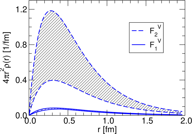
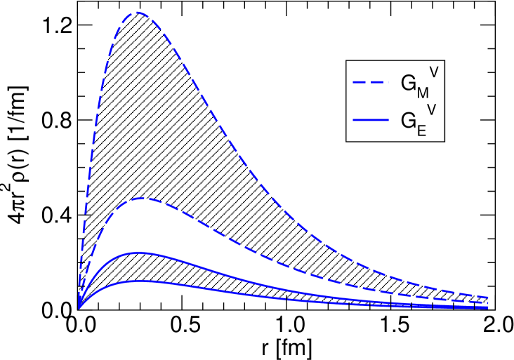
Figure 4: The densities of charge and magnetization due to the pion cloud. Left panel: $4\pi r^{2}\rho(r)$ for the isovector Pauli (upper band) and Dirac (lower band) form factors. Right panel: $4\pi r^{2}\rho(r)$ for the isovector magnetic (upper band) and electric (lower band) Sachs form factors.

In Fig. 4, we show the resulting densities for the isovector form factors weighted with $4\pi r^{2}$. The contribution of the “pion cloud” to the total charge or magnetic moment is then simply obtained by integration over $r$. The bands reflect the theoretical uncertainty in the separation. For all form factors, the lower and upper bounds are given by methods (b) and (a), respectively. Method (c) generally yields a result between these bounds, except for the Dirac form factor where it gives the upper bound. The weighted densities for the isovector Dirac and Pauli form factors are shown in the left panel of Fig. 4. We see that these charge distributions show a pronounced peak around $r\simeq 0.3\,$fm, quite consistent with earlier determinations (see e.g. UGM ; Holz ), and fall off smoothly with increasing distance. In the right panel of Fig. 4, we show the densities (again weighted with $4\pi r^{2}$) for the electric and magnetic Sachs form factors which come out very similar to the case of the Dirac and Pauli form factors. In comparison with Ref. FW , we generally obtain much smaller pion cloud effects at distances beyond 1 fm, e.g., by a factor 3 for $\rho_{E}^{V}(r)$ at $r=1.5$ fm. We have also studied the sensitivity of our results to the cut–off $t_{\rm{max}}$. While this may increase the value of the “pion cloud” contribution, it leaves the position of the maximum essentially unchanged. However, it is obvious from Eq. (10) that masses beyond 0.5 GeV and corresponding small–distance phenomena ($r\leq 0.4$ fm) should not be related to the pion cloud of the nucleon. Finally, we show the corresponding two–pion contribution to the charges and radii for the various nucleon form factors in Table 1. The contribution of the pion cloud to the isovector electric (magnetic) charge is 20% (10%) in the model of Ref. FW . This is consistent with our range of values for the electric charge but a factor of 1.5 smaller than our lower bound for the magnetic one, see Table 1. Furthermore, note that the pion cloud gives only a fraction of all form factors at zero momentum transfer. Normalized to the contribution of the pion cloud, the corresponding radii are of the order of 1 fm. In the model of FW , these radii are considerably larger, of the order of 1.5 fm. Note that if one shifts all the strength of the corresponding spectral functions to threshold, one obtains an upper limit $r_{\rm max}=\sqrt{3/2}\,M_{\pi}^{-1}\simeq 1.7\,$fm, assuming that the spectral functions are positive definite.

Table 1: Two–pion contribution to charges and radii (in fm²) for the various nucleon form factors. The radii are normalized to the physical charges and magnetic moments.

$F_{1}^{V}(0)$	$F_{2}^{V}(0)$	$G_{E}^{V}(0)$	$G_{M}^{V}(0)$	$\langle r^{2}\rangle_{1}^{V}$	$\langle r^{2}\rangle_{2}^{V}$	$\langle r^{2}\rangle_{E}^{V}$	$\langle r^{2}\rangle_{M}^{V}$
$0.07...0.08$	$0.4...1.0$	$0.1...0.2$	$0.4...1.0$	$0.1...0.2$	$0.2...0.3$	$0.2...0.3$	$0.2...0.3$

6 What can we conclude?

Let me summarize the pertinent conclusions of this talk:

• Chiral perturbation theory is the natural framework to investigate the role of pionic contributions to hadron (nucleon) structure. Nucleon observables receive contributions from pion loops, the “pion cloud“.

• In general at any given order in the chiral expansion beyond tree level, S-matrix elements and transition currents receive contributions from pion loops and local short-distance operators. Both these contributions are in general scale-dependent and thus it is possible to shuffle strength from one to the other. Consequently, an unambiguous extraction of the pion cloud contribution is not possible.

• The spectral functions that parameterize the physics of the isovector and isoscalar nucleon electromagnetic form factors are dominated for low masses by two- and three-pion exchanges, respectively. The two-pion contribution can be exactly worked out up to approximately 1 GeV by unitarity in terms of $\pi N$ scattering amplitudes and the pion vector form factor. The CHPT representation shares the same analytic properties, namely the strong enhancement on the left shoulder of the $\rho$ due to an anomalous threshold on the second sheet close to the physical threshold. A similar anomalous threshold effect in the isoscalar spectral functions is washed out by phase space factors. These constraints must be included in any serious analysis of the nucleon form factors.

• A model-dependent separation of the correlated from the uncorrelated two-pion exchange allows one to analyze the spatial extent of this longest range contribution to the isovector form factors. It is much more confined in space than in the analysis of Ref. FW .

• Concerning low momentum transfer bump-dip structures in the nucleon form factors for low $Q^{2}$, one should first realize that such structures have already been present in most dispersive analyses in the magnetic form factors. The novel structure in $G_{E}^{n}(Q^{2})$ proposed in Ref. FW can only be explained with spectral functions that contain additional light mass poles violating the strictures from unitarity and chiral symmetry as discussed above. According to the newest dispersive analysis BHMff , this bump-dip structure lies completely within the one sigma uncertainty and it requires an additional isoscalar/isovector pole close to the $\omega$/three-pion threshold. For a more detailed discussion on this topic, I refer to Ref. Hammer:2006mw .

References

- (1) H. Yukawa, Proc. Math.-Phys. Soc. Japan 17, 48 (1935).
- (2) H. Fröhlich, W. Heitler and N. Kemmer, Proc. Roy. Soc. A 166 , 155 (1938).
- (3) V. Bernard and U.-G. Meißner, Ann. Rev. Nucl. Part. Sci. 57 (2007) in print [hep-ph/0611231].
- (4) H. Georgi, Ann. Rev. Nucl. Part. Sci. 43, 209 (1993).
- (5) D. Espriu and J. Matias, Nucl. Phys. B 418, 494 (1994) [arXiv:hep-th/9307086].
- (6) G. Ecker, J. Gasser, A. Pich and E. de Rafael, Nucl. Phys. B 321, 311 (1989).
- (7) G. Ecker, J. Gasser, H. Leutwyler, A. Pich and E. de Rafael, Phys. Lett. B 223, 425 (1989).
- (8) J. F. Donoghue, C. Ramirez and G. Valencia, Phys. Rev. D 39, 1947 (1989).
- (9) K. Kampf and B. Moussallam, Eur. Phys. J. C 47, 723 (2006) [arXiv:hep-ph/0604125].
- (10) V. Bernard, T. R. Hemmert and U.-G. Meißner, Nucl. Phys. A 732, 149 (2004) [arXiv:hep-ph/0307115].
- (11) P. Mergell, U.-G. Meißner and D. Drechsel, Nucl. Phys. A 596, 367 (1996) [arXiv:hep-ph/9506375].
- (12) W. R. Frazer and J. R. Fulco, Phys. Rev. Lett. 2, 365 (1959).
- (13) G. Höhler and E. Pietarinen, Nucl. Phys. B 95, 210 (1975).
- (14) G. Höhler, ”Pion-Nucleon Scattering”, Landolt-Börnstein Vol. I/9b, ed. H. Schopper, Springer, Berlin, 1983.
- (15) R. R. Akhmetshin et al. [CMD-2 Collaboration], Phys. Lett. B 527, 161 (2002) [arXiv:hep-ex/0112031]; Phys. Lett. B 578, 285 (2004) [arXiv:hep-ex/0308008].
- (16) A. Aloisio et al. [KLOE Collaboration], Phys. Lett. B 606, 12 (2005) [arXiv:hep-ex/0407048].
- (17) M. N. Achasov et al., J. Exp. Theor. Phys. 101, 1053 (2005) [Zh. Eksp. Teor. Fiz. 101, 1201 (2005)] [arXiv:hep-ex/0506076].
- (18) M. A. Belushkin, H. W. Hammer and U.-G. Meißner, Phys. Lett. B 633, 507 (2006) [arXiv:hep-ph/0510382].
- (19) G. Höhler and E. Pietarinen, Phys. Lett. B 53, 471 (1975).
- (20) J. Gasser, M. E. Sainio and A. Svarc, Nucl. Phys. B 307, 779 (1988).
- (21) V. Bernard, N. Kaiser and U.-G. Meißner, Int. J. Mod. Phys. E 4, 193 (1995) [arXiv:hep-ph/9501384].
- (22) V. Bernard, N. Kaiser and U.-G. Meißner, Nucl. Phys. A 611, 429 (1996) [arXiv:hep-ph/9607428].
- (23) N. Kaiser, Phys. Rev. C 68, 025202 (2003) [arXiv:nucl-th/0302072].
- (24) B. Kubis and U.-G. Meißner, Nucl. Phys. A 679, 698 (2001) [arXiv:hep-ph/0007056].
- (25) M. R. Schindler, J. Gegelia and S. Scherer, Eur. Phys. J. A 26, 1 (2005) [arXiv:nucl-th/0509005].
- (26) K. de Jager, arXiv:nucl-ex/0612026.
- (27) H. W. Hammer, U.-G. Meißner and D. Drechsel, Phys. Lett. B 385, 343 (1996) [arXiv:hep-ph/9604294].
- (28) H. W. Hammer and U.-G. Meißner, Eur. Phys. J. A 20, 469 (2004) [arXiv:hep-ph/0312081].
- (29) M. A. Belushkin, H. W. Hammer and U.-G. Meißner, Phys. Rev. C (2007) in print; arXiv:hep-ph/0608337.
- (30) C. Adamuscin, S. Dubnicka, A. Z. Dubnickova and P. Weisenpacher, Prog. Part. Nucl. Phys. 55, 228 (2005) [arXiv:hep-ph/0510316].
- (31) R.J. Eden, P.V. Landshoff, D.I. Olive and J.C. Polkinghorne, The Analytic S–Matrix (Cambridge University Press, Cambridge, 1966).
- (32) H. W. Hammer, D. Drechsel and U.-G. Meißner, Phys. Lett. B 586, 291 (2004) [arXiv:hep-ph/0310240].
- (33) V. Bernard, N. Kaiser and U.-G. Meißner Nucl. Phys. A 615, 483 (1997) [arXiv:hep-ph/9611253].
- (34) U.-G. Meißner, Comm. Nucl. Part. Phys. 20, 119 (1991).
- (35) U.-G. Meißner, Phys. Rept. 161, 213 (1988).
- (36) G. Holzwarth, Z. Phys. A 356, 339 (1996) [arXiv:hep-ph/9606336].
- (37) J. Friedrich and T. Walcher, Eur. Phys. J. A 17, 607 (2003) [arXiv:hep-ph/0303054].
- (38) H. W. Hammer, Eur. Phys. J. A 28, 49 (2006) [arXiv:hep-ph/0602121].