Random Matrices and Chaos in Nuclear Spectra

Abstract

We speak of chaos in quantum systems if the statistical properties of the eigenvalue spectrum coincide with predictions of random–matrix theory. Chaos is a typical feature of atomic nuclei and other self–bound Fermi systems. How can the existence of chaos be reconciled with the known dynamical features of spherical nuclei? Such nuclei are described by the shell model (a mean–field theory) plus a residual interaction. We approach the question by using a statistical approach (the two–body random ensemble): The matrix elements of the residual interaction are taken to be random variables. We show that chaos is a generic feature of the ensemble and display some of its properties, emphasizing those which differ from standard random–matrix theory. In particular, we display the existence of correlations among spectra carrying different quantum numbers. These are subject to experimental verification.

I Random Matrices and Chaos

I.1 Introduction

This paper contains a colloquium talk on the application of random matrices to nuclear spectroscopy. We discuss the origin of random–matrix theory (RMT), some of its predictions, and its relation to classical chaos. We show that the predictions of RMT often agree very well with spectroscopic data in nuclei. In the main part of the paper, we address the question: How can this success of RMT be reconciled with our knowledge of the dynamical behavior of nuclei as embodied in the nuclear shell model? Although actually formulated for nuclei, we believe that our arguments apply likewise in modified form to other Fermi systems like atoms and molecules.

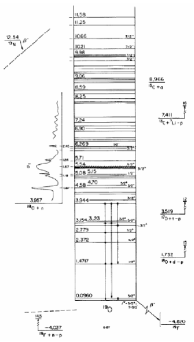
Near the ground state, the spectra of self–bound Fermi systems are essentially discrete. As an example, Fig. 1 shows the measured spectrum of the nucleus ¹⁹O. Up to the threshold for decay into a neutron (n) and ¹⁸O (the “neutron threshold”) at an excitation energy of 3.957 MeV, the levels shown decay only by gamma emission; the ground state is unstable against beta decay. The long lifetimes of these decay modes render the levels virtually discrete. Above neutron threshold, the levels acquire finite particle decay widths (which typically are much larger than those for beta and gamma decay) and are also seen as resonances in cross sections (like in the one for the reaction n + ¹⁸O). The levels in Fig. 1 carry quantum numbers which reflect symmetries of the nuclear Hamiltonian: Total spin $J$ corresponds to rotational invariance, total isospin $T$ to proton–neutron symmetry, parity $P$ to mirror reflection symmetry. In heavy nuclei, the Coulomb interaction between protons breaks the isospin quantum number. In its general appearance, Fig. 1 is representative not only for nuclei but also for atoms, molecules, and atomic clusters.

Figure 1: The spectrum of ¹⁹0. Taken from Ref. Ajz87 .

I.2 Regular Motion

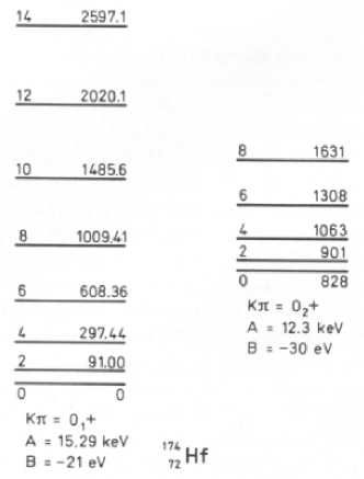
The excitation energies and widths for beta, gamma, and particle decay of the levels found experimentally can often be successfully described in terms of simple integrable dynamical models. In analogy to classical mechanics, we then speak of regular motion. A striking example is furnished by the existence of rotational bands. These are characterized by a spin/parity $J^{P}$ sequence $0^{+},2^{+},4^{+},\ldots$ and excitation energies proportional to $J(J+1)$. They correspond to a rotation of the entire (non–spherical) nucleus about some axis. Fig. 2 shows two such bands in the nucleus ¹⁷⁴Hf. Another example for regular motion is provided by the independent–particle model: nucleons move independently in the mean field of the nucleus. This model corresponds to the most elementary version of the nuclear shell model and accounts for the existence of “magic numbers” for neutrons and protons (i.e., numbers where a major shell is filled and where the nuclear binding energy attains maxima) as well as for spins and parities of ground states of nuclei differing by one unit in proton or neutron number from closed–shell nuclei. We discuss the nuclear shell model in more detail in the next Section.

Figure 2: Rotational bands in ¹⁷⁴Hf. Taken from Ref. Boh .

I.3 Non–regular Motion

The emphasis in this paper is on chaotic motion in nuclei. The previous Subsection serves as a reminder that there is strong evidence for regular motion in nuclei, especially in the vicinity of the ground state. We now turn to the equally strong evidence for chaotic motion. We put the argument in the form of a semi–historical narrative which will occupy the remainder of this Subsection.

The first evidence for chaotic motion in nuclei came from spectroscopic data on levels at neutron threshold, i.e., rather far from the ground state. In general, it is exceedingly difficult to unambiguously identify the positions, spins, and parities of such levels. Neutron time–of–flight spectroscopy offers the unique opportunity to acquire precise spectroscopic information in a range of excitation energies which is otherwise virtually inaccessible. The neutron threshold in medium–mass and heavy nuclei typically occurs at an excitation energy of 8 to 10 MeV (and not at $\approx$ 4 MeV as in ¹⁹O, see Fig. 1). Measuring the total cross section for slow neutrons versus kinetic energy, one observes resonances. Each of the resonances corresponds to a nuclear state at an excitation energy of around 8 or 10 MeV. The ground states of even–even nuclei have spin/parity $0^{+}$. Slow neutrons carry angular momentum zero and have spin $1/2$. For even–even target nuclei, the states seen, therefore, all have spin/parity $1/2^{+}$. We show here not the earliest but some of the best data. In the 1970s, the Columbia group around Rainwater measured time–of–flight spectra of slow neutrons scattered on a number of heavy nuclei. For each target nucleus, they observed a sequence of up to 200 $1/2^{+}$ levels. (That number was limited by the resolution of the time–of–flight spectrometer.) Fig. 3 shows their data for the total neutron scattering cross section on ²³⁸U versus neutron energy. We see a number of very narrow resonances (widths typically smaller than 1 eV) with typical spacings of 10 eV. The energies of the associated levels were determined with the help of an $R$–matrix multi–level analysis Lane .

Figure 3: Total cross section for scattering of neutrons by ²³⁸U versus neutron energy. Taken from Ref. Rain .

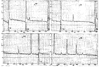
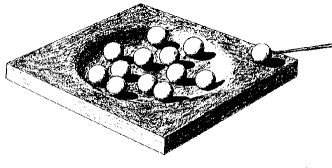
Already in the 1930s, similar data (of much inferior quality) had led N. Bohr to formulate his “compound nucleus hypothesis” NBohr . Bohr argued that the existence of narrowly spaced narrow resonances is incompatible with independent–particle motion in the nucleus. Indeed, simple estimates using a central potential yield single–particle $s$–wave level spacings around 1 MeV (and not 10 eV as shown in Fig. 3), and $s$–wave decay widths for neutron–instable states of around 100 keV (and not $<$ 1 eV as shown in Fig. 3). Bohr argued that the existence of such narrow resonances could not be understood without assuming strong interactions between the incident neutron and the nucleons in the target. A wooden toy model (shown in Fig. 4) was to demonstrate this idea of the compound nucleus. The billiard balls represent nucleons, the queue indicates the kinetic energy of the incident neutron, and the trough simulates the attractive mean field. Since the publication of N. Bohr’s 1937 paper and until the discovery of the nuclear shell model in 1949, the idea of independent–particle motion in the nucleus was virtually inacceptable in the nuclear physics community. And as we shall see, understanding chaos in nuclei is almost synonymous to reconciling N. Bohr’s idea of the compound nucleus with the nuclear shell model.

Figure 4: Wooden toy model simulating N. Bohr’s compound nucleus. Taken from Ref. NBohr1 .

I.4 Random Matrices

When Wigner Wign introduced random matrices into physics, he did not refer explicitly to N. Bohr’s 1937 paper NBohr . Nevertheless we believe that his work was motivated by and can be seen as the mathematical formulation of the idea of the compound nucleus. It is noteworthy that the work started in 1951, two years after the discovery of the shell model.

How can one deal with a situation where the constituents of a quantum system interact strongly? We suppose that we deal with a non–integrable system without remaining symmetries. By that we mean that extant symmetries of the Hamiltonian like total spin and parity have been taken into account; the Hamiltonian has block–diagonal form; the individual blocks are free of further symmetries; we focus attention on one such block to which we refer for simplicity as the Hamiltonian. Is it possible to make generic statements about the spectrum and eigenvalues of such a system? Following Wigner Wign , we consider the matrix representation $H_{\mu\nu}$ of the Hamiltonian in Hilbert space. Here $\mu,\nu=1,\ldots,N$ and $N\gg 1$ (we let $N\to\infty$ at the end of the calculation). Nuclei are time–reversal invariant. Therefore, we can choose a representation where $H_{\mu\nu}$ is real and symmetric. There are no further symmetries beyond rotational symmetry and parity. Now comes the decisive and unusual step: Rather than considering the individual Hamiltonian of the actual physical system, we study an entire ensemble of Hamiltonians all having the same symmetry. It turns out that while we cannot make generic statements about the individual Hamiltonian, such statements are possible about almost all members of the ensemble.

The ensemble is defined in such a way that it combines generality with the symmetry of $H$: It consists of real and symmetric matrices. To avoid a preferred direction in Hilbert space, it is chosen to be invariant under those transformations in Hilbert space which preserve the symmetry of $H$. These are the orthogonal transformations. The ensemble is defined in terms of a probability density in matrix space. That density has the form

$$C\exp\bigg{(}-\frac{N\ {\rm trace}(H^{2})}{\lambda^{2}}\bigg{)}\prod_{\mu\leq\nu}{\rm d}H_{\mu\nu}$$ (1)

The last factor is the product of the differentials of the independent matrix elements. That factor is orthogonally invariant, and so is the trace of $H^{2}$ in the exponent. The Gaussian factor is introduced because a cutoff is needed to render the integrals over matrix space convergent. The ensemble is characterized by a single parameter $\lambda$, which has the dimension of energy. This parameter determines the mean level spacing of the ensemble, i.e., the mean value of the distance between two neighboring eigenvalues. We will be interested in the fluctuations of the spacings of neighboring levels around that mean value, and in the correlations between spacings of different pairs of neighboring levels. These are characterized by certain local fluctuation measures which are introduced below. All measures depend on the level spacing expressed in units of the mean level spacing and are, therefore, independent of the parameter $\lambda$ and altogether parameter–free. The factor $C$ is a normalization factor. The factor $N$ in the exponent (with $N$ the matrix dimension) guarantees that the spectrum has finite range. Expression (1) defines the Gaussian orthogonal ensemble (GOE) of random matrices. Dyson dys showed that there are three canonical random–matrix ensembles defined by symmetry: the GOE, the Gaussian unitary ensemble (GUE) (for time–reversal non–invariant systems), and the Gaussian symplectic ensemble (GSE) (for systems with half–integer spin which are not rotationally invariant). GUE, GOE, and GSE carry the Dyson parameters $\beta=1,2,$ and $4$, respectively.

While the symmetry of the Hamiltonian and, thus, the form of the invariant measure in expression (1) is dictated by quantum mechanics, the choice of the Gaussian cutoff is arbitrary and dictated by convenience. It has been shown, however, that an entire class of different choices (like, for instance, taking the trace of the fourth power of $H$ in the exponent) yields the same results for the local fluctuation measures. This important property is referred to as universality of the ensemble. It guarantees that the local fluctuation measures predicted by the GOE are generic.

Random–matrix theory (RMT) only predicts ensemble averages of observables (calculated by integrating the observable over the ensemble (1)). But experimentally, we always deal with a single Hamiltonian, not an ensemble. The applicability of RMT to a single system is guaranteed by the property of ergodicity: For almost all members of the ensemble, the ensemble average of an observable (as given by RMT) is equal to the running average of that observable taken over the spectrum of a single member. Ergodicity guarantees that the quantitative and parameter–free predictions of RMT can be meaningfully compared with experimental data.

I.5 Fluctuation Measures

The two fluctuation measures most frequently employed in analyzing data are the nearest–neighbor spacing (NNS) distribution and the Dyson–Mehta or $\Delta_{3}$ statistic. Fig. 5 gives the NNS distribution $P_{\beta}(s)$, i.e., the probability distribution of spacings, versus $s$ (the actual spacing of two neighboring eigenvalues in units of their mean spacing) for Dyson’s three canonical ensembles. The distributions are characterized by level repulsion at short distances ($P_{\beta}(s)\propto s^{\beta}$ for small $s$) and a Gaussian falloff for large $s$. We note that if the system were integrable, all eigenvalues would carry different quantum numbers, and level repulsion were absent. The $\Delta_{3}$ statistic measures correlations between eigenvalue spacings. Let ${\cal N}(E)$ denote the total number of levels below energy $E$. Clearly ${\cal N}(E)$ is a step function which increases by one unit as $E$ passes an eigenvalue. The $\Delta_{3}$ statistic measures how well ${\cal N}(E)$ is on average approximated by a straight line. It is defined by

$$\Delta_{3}(L)=\bigg{\langle}{\rm min}_{a,b}\frac{1}{L}\int_{E_{0}}^{E_{0}+L}\ \bigg{(}{\cal N}(E^{\prime})-aE^{\prime}-b\bigg{)}^{2}{\rm d}E^{\prime}\bigg{\rangle}_{E_{0}}\ .$$ (2)

Minimization with respect to $a$ and $b$ determines the best straight line. The angular brackets denote an average over the initial energy $E_{0}$ and over the ensemble. All energies are in units of the mean level spacing, and $\Delta_{3}(L)$ is, therefore, parameter free. If the spacings were totally uncorrelated, then $\Delta_{3}$ would be linear in $L$. It would grow much less fast with $L$ if the spacings were correlated in such a way that a large spacing is always followed by a small one and vice versa. The actual behavior of $\Delta_{3}(L)$ is shown as a solid line in Fig. 7: $\Delta_{3}(L)$ grows essentially logarithmically with $L$. This property is referred to as the “stiffness” of RMT spectra.

Figure 5: The nearest–neighbor spacing distribution $P_{\beta}(s)$ versus $s$, the actual spacing in units of the mean level spacing, for the three canonical ensembles with $\beta=1,2,4$ (solid, dashed, and dotted lines). $\beta=2$ corresponds to the GOE. Taken from Ref. TG .

For our later discussion, it is important to note that a GOE spectrum does not carry any information content beyond the mean level spacing. This is obvious since any realization of $H$ is obtained by drawing random numbers from the Gaussian distribution (1). Thus, it would be useless to apply spectroscopic analyses to such a spectrum. Put differently, a GOE Hamiltonian has $N(N+1)/2$ independent matrix elements. Counting shows that we need to measure all $N$ eigenvalues and all $N$ eigenfunctions to reconstruct $H$. This is very different for typical dynamical systems where the Hamiltonian is known except for a small number of parameters.

I.6 Quantum Chaos

Suppose the fluctuation measures of an experimental spectrum agree with GOE predictions. What does such a result imply physically? The understanding of this question was much advanced by the study of few–degrees–of–freedom quantum systems which are chaotic in the classical limit. The development culminated in the Bohigas–Giannoni–Schmit conjecture Bohi . It says: The spectral fluctuation properties of a quantum system which is chaotic in the classical limit, coincide with those of the canonical random–matrix ensemble that has the same symmetry. The authors of Ref. Bohi supported their conjecture by calculating numerically the NNS distribution and the $\Delta_{3}$ statistic for the Sinai billiard, a system which is time–reversal invariant and fully chaotic in the classical limit, and comparing the result with the GOE prediction. This is shown in Figs. 6 and 7.

Figure 6: The NNS distribution for the Sinai billiard (histogram) and the GOE prediction (solid line). Taken from Ref. Bohi .

Figure 7: The $\Delta_{3}$ for the Sinai billiard (histogram) and the GOE prediction (solid line). Taken from Ref. Bohi .

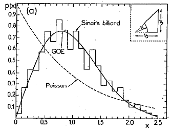
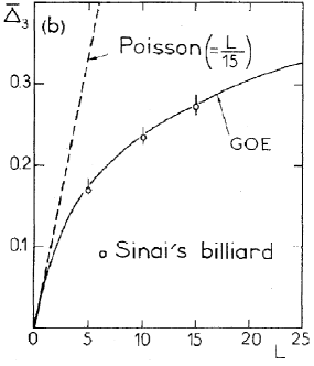
Agreement like the one shown in Figs. 6 and 7 has since been found in many other chaotic systems. Moreover, an analytical proof of the Bohigas–Giannoni–Schmit conjecture has recently been published heusler . That proof uses the semiclassical approximation and generic properties of chaotic trajectories. We are, thus, led to consider agreement between the spectral fluctuations of a physical system and RMT predictions as a signal for chaotic motion. It is in that sense that we will use the word chaos also in nuclei. This is done with a caveat: The semiclassical proof in Ref. heusler is not applicable directly to nuclei because nuclei are too dense to admit a semiclassical approximation.

Quantum chaos has been studied intensely during the last 20 years or so haake . These studies have focused mainly on dynamical systems with few degrees of freedom. The Sinai billiard is a prime example. Here chaos is due to the fact that the inner circle and the outer rectangle possess incommensurate symmetries. In contradistinction, the atomic nucleus is a many–body system. We will show that in such a system, the dynamical features which cause chaos are distinctly different from the ones which cause chaos in few–degrees–of–freedom systems.

I.7 Chaos in Nuclei

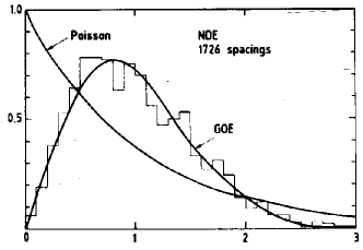
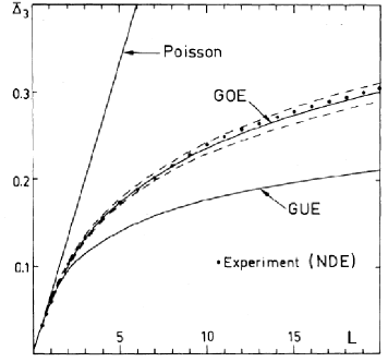
Now we are in the position to return to the data shown in Fig. 3. Combining the information on the excited levels in ²³⁹U obtained from these data with that of many similar experiments on the scattering of slow neutrons and of protons at the Coulomb barrier by other nuclei, Haq, Pandey, and Bohigas Haq formed the “nuclear data ensemble”. It consists of 1726 spacings. These were used to determine the NNS distribution and the $\Delta_{3}$ statistic. The results are shown in Figs. 8 and 9. The solid lines labeled “Poisson” correspond to totally uncorrelated levels and, thus, to integrable systems. The agreement with the GOE prediction is impressive. We conclude that at neutron threshold (and at the Coulomb barrier for protons) nuclei display chaotic motion. The deep physical insight of N. Bohr, who conceived the idea of the compound nucleus and who designed the wooden model of Fig. 4, is borne out by the data: Idealized models of billiards are prime examples of chaotic motion, and nuclear levels at neutron threshold display chaotic behavior. Since 1983, there has been growing evidence for chaotic motion in nuclei also at lower excitation energies, although the statistics of such data is usually not as good as near neutron threshold.

Figure 8: The NNS distribution for the nuclear data ensemble (histogram) and the GOE prediction (solid line). Taken from Ref. Haq .

Figure 9: The $\Delta_{3}$ for the nuclear data ensemble (data points) and the GOE prediction (solid line). Taken from Ref. Haq .

In conclusion, there is strong evidence for chaotic motion in nuclei. How can this evidence be reconciled with the extant information on nuclear dynamics (the shell model)? And – given the fact that GOE spectra carry zero information content beyond the mean level spacing – which is the information content of nuclear spectra in the regime of chaotic motion? These are the questions we address in the remainder of this paper.

II Dynamical Aspects

II.1 Chaos in the Nuclear Shell Model

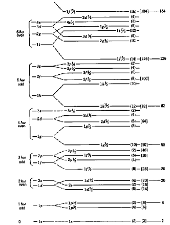
The shell model is the universal model for the structure of atoms and nuclei. In nuclei, it consists of a central potential $U$ with a strong spin–orbit interaction (the “mean field”) and a fairly weak “residual interaction” $V$ which accounts for the remaining part of the nucleon–nucleon interaction. The central potential $U$ defines the major shells shown in Fig. 10: The $1s$–shell, the $1p$–shell, the $2s1d$–shell, etc. in spectroscopic notation, the latter with the subshells $s_{1/2}$, $d_{3/2}$ and $d_{5/2}$ where the indices denote the nucleon spin. The subshells have different single–particle energies and the states within a major shell are, therefore, not totally degenerate. Still, large degeneracies remain when the shell contains more than a single nucleon. These degeneracies are lifted by the residual interaction $V$. That interaction conserves parity and is rotationally invariant and invariant under time reversal. It is weak in the sense that it produces configuration mixing primarily within the same major shell. More precisely: The magnitude of a typical matrix element is small compared with the spacing of the centroids of adjacent major shells but comparable with that of adjacent subshells in the same major shell. In all that follows we will, therefore, consider only a single major shell. And the residual interaction is predominantly a two–body interaction, $V=\sum_{\alpha<\beta}V(\vec{r}_{\alpha},\vec{r}_{\beta})$ although there is evidence that three–body forces are needed to obtain quantitative agreement with experimental spectra. Again, we will confine ourselves for simplicity to two–body forces.

Figure 10: Level sequence in the nuclear shell model. Taken from Ref. May .

The Hamiltonian of the shell model is

$$H=\sum_{\alpha}\left(-{\hbar^{2}\over 2m}\Delta_{\alpha}+U(\vec{r}_{\alpha})\right)+\sum_{\alpha<\beta}V(\vec{r}_{\alpha},\vec{r}_{\beta})\ .$$ (3)

Here, $\vec{r}_{\alpha}$ denotes the coordinates and spin/isospin degrees of freedom of the nucleon labeled $\alpha$. The single–particle part of $H$ has eigenstates $|j\rangle$ and eigenvalues $\varepsilon_{j}$. We use second quantization and write $H$ as

$$H=\sum_{j}\varepsilon_{j}a^{\dagger}_{j}a_{j}+{1\over 4}\sum_{ijkl}v(ij;kl)a^{\dagger}_{i}a^{\dagger}_{j}a_{l}a_{k}\ .$$ (4)

Here, $a_{j}^{\dagger}$ creates a nucleon in a single-particle state $j$. The two–body matrix elements $v(ij;kl)$ represent the residual interaction. In writing Eq. (4) we have not paid attention to conserved quantum numbers like spin and isospin. This was done in order to keep the notation simple. More details concerning this aspect are given in Section II.2.

In the shell model it is assumed that all shells but one are completely filled, and attention is focused on that last shell (the “valence shell”). Distributing the valence nucleons over the various subshells in the valence shell, one constructs a basis of antisymmetrized many–body states $|J\mu\rangle$. We use a short–hand notation where $J$ stands for total spin, total isospin, and parity, while $\mu$ is a running index. These are used to calculate the matrix elements

$$H_{\mu\nu}(J)=\langle J\mu|H|J\nu\rangle$$ (5)

of the Hamiltonian (4) in the subspace with quantum numbers $J$. Diagonalization of $H_{\mu\nu}(J)$ yields the eigenvalues and eigenfunctions. The latter are used to calculate various transition matrix elements. This scheme has been used with considerable success in many parts of the periodic table. Exceptions are mainly deformed nuclei which occur in the middle between large major shells. When we refer to Eq. (4) in the text further below, we always do so with the understanding that that equation refers to the valence shell only.

In the sequel we focus attention to the $2s1d$–shell (in short: the $sd$–shell). The $1s$–shell and the $1p$–shell are filled, taking a total of 16 nucleons. Thus, the $sd$–shell describes nuclei with mass numbers between 16 (O) and 40 (Ca). We do so for practical reasons: The dimensions of the Hamiltonian matrices in the $sd$–shell are quite manageable (maximal dimensions are of the order of $10^{3}$) while much larger numbers occur in higher shells. We sometimes consider also a single $j$–shell with half–integer $j$. Although not realistic in the framework of the nuclear shell model, this idealization is useful for purposes of orientation.

Which are the fluctuation properties of the resulting spectra? That question was studied, for instance, in Ref. Zel . The authors used standard single–particle energies and a standard two–body residual interaction to calculate the positions of the states with spin $J=2$ and isospin $T=0$ for 12 nucleons in the $sd$–shell. The matrix dimension is 874. In Figs. 11 and 12, the NNS spacing distribution and the $\Delta_{3}$ statistic for these levels are compared with GOE predictions. The agreement is very good. (It would be desirable to confirm this result experimentally. Unfortunately, the data needed are not available: There is no more than a handful of levels known for each value of spin and isospin; such levels cluster in the vicinity of the ground state). In Ref. Zel numerous further results (on thermodynamic properties, on the statistics of eigenfunctions etc.) were described. While it was found that the input used in shell–model calculations (the distribution of many–body matrix elements) differs from that used in the GOE, the results agree to a very large extent with GOE predictions.

Figure 11: NNS spacing distribution for the $J=2,T=0$ states of 12 nucleons in the $sd$–shell (histogram) compared to the GOE (line). Taken from Ref. Zel .

Figure 12: $\Delta_{3}$ statistic for the $J=2,T=0$ states of 12 nucleons in the $sd$–shell (data points) compared to the GOE (solid line). Taken from Ref. Zel .

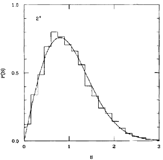
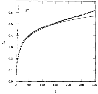
The result displayed in Figs. 11 and 12 and the other results obtained on chaos in shell–model calculations are surprising and call for a deeper analysis. Indeed, the Hamiltonian of the shell model is quite different from a GOE matrix. And yet, it is able to produce GOE–like spectral fluctuations! It does not seem unreasonable to speculate that the shell model would also be able to account for the GOE–like spectral fluctuations shown in Figs. 8 and 9 (this cannot be checked because of the huge dimensions of the matrices involved). At the same time, the shell model accounts well for some of the regular features observed experimentally like magic numbers and spectroscopic data on low–lying states. The questions raised at the end of Subsection I.7 must, therefore, be reformulated as follows: Are the results shown in Figs. 11 and 12 a generic property of the shell model or are they due to very special circumstances? In other words: How is chaos produced in the shell model? And what is the information content of shell–model spectra? A further question would be: How does the shell model manage to produce both regularity and chaos? We will not address that last question. Suffice it to say that regularity is mostly seen when we consider states with different quantum numbers like in Fig. 2, while chaos is manifest in long sequences of states carrying identical quantum numbers. The way we use them here, regularity and chaos are not neccessarily contradictory concepts.

II.2 Two–body Random Ensemble (TBRE)

To answer these questions, it is neccessary to go somewhat more deeply into the details of shell–model calculations. The single–particle states in the shell model carry the half–integer spin quantum number $j$. The two–body interaction scatters a pair of nucleons in states $(j_{1},j_{2})$ into states $(j_{3},j_{4})$ which may or may not be identical to $(j_{1},j_{2})$. The two–body interaction conserves total spin, total isospin, and parity. Coupling the initial and the final pair of states to total spin $s$ (and suppressing the analogous coupling for isospin for simplicity), we write the antisymmetrized reduced matrix elements of the two–body interaction in the form $\langle j_{3}j_{4}s|V|j_{1}j_{2}s\rangle$ or, more simply, as $v(\alpha)$ where the index $\alpha$ labels different two-body matrix elements. (The word “different” refers to matrix elements not connected by symmetry properties.) Counting (which must include spin and isospin) shows that in the $sd$–shell, $\alpha$ ranges from $1$ to $63$, and in a single $j$–shell with half–integer $j$, from $1$ to $j+1/2$.

Chaos has to do with the complete mixing of states in Hilbert space. How does the residual interaction accomplish such mixing? We focus attention on the two–body interaction and assume that all subshells belonging to a major shell are degenerate. (It is intuitively obvious and has been shown numerically that the mixing of shell–model states becomes weaker as the differences between single–particle energies of subshells become comparable to the magnitudes of the $v(\alpha)$.) We accordingly omit the single–particle energies in Eq. (4) altogether. The Hamiltonian $H_{\mu\nu}$ of Eq. (5) is then completely determined by the two–body interaction in Eq. (4). Thus, it has the form

$$H_{\mu\nu}(J)=\sum_{\alpha}v(\alpha)\ C_{\mu\nu}(J,\alpha)\ .$$ (6)

The sum over $\alpha$ is equivalent to the sum over $\{ijkl\}$ in Eq. (4). Each term in the sum in Eq. (6) is the product of two contributions. The $v(\alpha)$ stand for the matrix elements denoted by $v(ij;kl)$ in Eq. (4) (except that we have now paid proper attention to the coupling of angular momenta) and represent the specific features of the two–body interaction. Except for angular momentum coupling coefficients, the elements of the coefficient matrices $C_{\mu\nu}(J,\alpha)$ are the matrix elements of the operators $a^{\dagger}_{i}a^{\dagger}_{j}a_{l}a_{k}$ in Eq. (4). These matrices are determined by the major shell we are in, by the coupling scheme we have chosen to construct the states $|J\mu\rangle$, and by the specific two–body interaction operator labeled $\alpha$ which defines the matrix element $v(\alpha)$. The matrices $C_{\mu\nu}(J,\alpha)$ represent the geometry and symmetries of the shell model and are generic in the sense that they are independent of the actual choice of the residual interaction. The seemingly trivial Eq. (6) actually contains very useful information about chaos in the shell model.

To answer the question “How does the residual interaction cause chaos?” in the most general terms, we wish to study the Hamiltonian (6) for the most general two–body interaction. This is accomplished by assuming that the elements $v(\alpha)$ of the two–body interaction are Gaussian–distributed random variables with mean value zero and a common second moment. The value of that moment is irrelevant since it determines only the overall scale of the spectrum. With this assumption, the matrices (6) form an ensemble of Gaussian–distributed random matrices. This is the two–body random ensemble (TBRE) of the shell model originally introduced in the 1970s by French and Wong Fre and by Bohigas and Flores Boh2 . The TBRE is tailored to the shell model and, therefore, much more realistic than the GOE. The ensemble being defined in terms of an integration over the Gaussian variables $v(\alpha)$, statements derived by averaging over the ensemble hold for all members of the ensemble with the exception of a set of measure zero with respect to that integration measure.

Within the TBRE, the $v(\alpha)$ play a minor role only: They determine the specific linear combination of the matrices $C_{\mu\nu}(J,\alpha)$ which forms the Hamiltonian. If the Hamiltonian causes chaos for almost all choices of the $v(\alpha)$, that property must be inherent in the matrices $C_{\mu\nu}(J,\alpha)$. Therefore, an analytic theory has to address these matrices as the fundamental building blocks of the TBRE. Unfortunately, such a theory is in its infancy as yet. An analytically more accesible ensemble is provided by the embedded Gaussian orthogonal ensemble EGOE($k$) Mon . This is defined as a random matrix ensemble of $m$ Fermions occupying $l$ degenerate single–particle levels with Gaussian–distributed random $k$-body interaction matrix elements, but assumes no further symmetries like spin and isospin. For $k=m$, the EGOE($k$) becomes the GOE, and for $k=2$, it becomes the analogue of the TBRE without quantum numbers. For recent reviews, we refer the reader to Refs. Kota ; Benet . Less is kown for the TBRE. In the sequel, we describe some insights that have been gained over the last few years.

II.3 Comparison GOE–TBRE

The GOE has three important properties: It is invariant under orthogonal transformations (hence, analytically tractable), it is universal, and it is ergodic. The TBRE probably does not share any of these properties. The set of matrices $C_{\mu\nu}(J,\alpha)$ is fixed. A unitary transformation of all matrices generates another representation of the ensemble but not another member of the ensemble. Therefore, the TBRE is not unitarily invariant. It is not clear how a non–Gaussian distribution of the $v(\alpha)$ would affect spectral fluctuation properties of the TBRE. In the case of the GOE, local fluctuation properties and global spectral properties become separated in the limit $N\to\infty$. That separation is at the root of universality (local fluctuation properties do not depend on the form of the distribution of the matrix elements). By definition, the TBRE is linked to a specific shell; its matrices have finite dimension. Similarly for ergodicity: For the GOE, that property is proved by showing that correlation functions vanish with increasing distance of their energy arguments. The proof uses the limit $N\to\infty$. This limit does not exist in the TBRE. One is tempted to ask: Why bother with the TBRE? The answer is: The TBRE is more realistic than the GOE. Moreover, it might be possible to study the TBRE analytically for the case of a single $j$–shell and to prove universality and ergodicity in the limit $j\to\infty$.

Except for the mirror symmetry about the main digonal, every element of a GOE Hamiltonian matrix stands for an independent random variable. For $N\gg 1$, the number $N(N+1)/2$ of such variables is much larger than the matrix dimension $N$. The number $n$ of independent random variables in the TBRE is typically small in comparison with the matrix dimension. For the case of a single $j$–shell, $n$ grows linearly with $j$ while the typical matrix dimension grows exponentially with $j$. In the GOE, the analogues of the matrices $C_{\mu\nu}(J,\alpha)$ exist. These are the $N(N+1)/2$ matrices ${G}_{\mu}$ which either have a unit element somewhere in the main diagonal and zeros everywhere else, or have a unit element somewhere above the main diagonal, its mirror image below, and zeros everywhere else. The set $\{G_{\mu}\}$ forms a complete basis for real and symmetric matrices. In contradistinction, the matrices $C_{\mu\nu}(J,\alpha)$ do not form such a complete set. To be sure, every matrix $C_{\mu\nu}(J,\alpha)$ may be thought of as a linear combination of the ${G}_{\mu}$. But the number of matrices $C_{\mu\nu}(J,\alpha)$ is typically much smaller than $N(N+1)/2$. Therefore, many other linear combinations of the ${G}_{\mu}$ exist which are linearly independent of the $C_{\mu\nu}(J,\alpha)$ and which do not occur in the TBRE. The TBRE may be negatively defined by constraining all such linear combinations to be zero.

We are going to present evidence that the matrices $C_{\mu\nu}(J,\alpha)$ are the agents which cause chaos in the TBRE. In anticipation of this result, we give a qualitative argument why every matrix $C_{\mu\nu}(J,\alpha)$ may be thought of as a single representation of the GOE. In constructing the many–body basis states $|J\mu\rangle$, we may proceed as follows. We form Slater determinants by distributing $m$ nucleons over the single–particle states of a major shell. These are antisymmetric by construction but do not possess good quantum numbers $J$. States with good $J$ are obtained as linear combinations of such Slater determinants, a typical state $|J\mu\rangle$ consisting of a linear combination of many determinants. Although the two–body interaction has non–vanishing matrix elements only between determinants that differ in the occupation numbers of not more than two single–particle states, that fact makes sure that the matrices $C_{\mu\nu}(J,\alpha)$ are densely filled. Moreover, the coefficients in the linear combinations are determined by angular–momentum algebra, i.e., contain Clebsch–Gordan coefficients, Racah coefficients, and coefficients of fractional parentage. Although individually determined group–theoretically, these quantities combine to make the coefficients of the linear combinations almost random numbers. This stochastic aspect of the shell model has been emphasized by Zelevinsky and collaborators who employed the term “geometric chaoticity” Zel .

Thus, the matrices $C_{\mu\nu}(J,\alpha)$ are dense and their elements are close to being random. Our qualitative argument is subject to two caveats. First, the dimension of the matrices $C_{\mu\nu}(J,\alpha)$ is always finite. Second, the matrices $C_{\mu\nu}(J,\alpha)$ are not dense everywhere and may have a substructure with blocks that are completely empty. Consider, for instance, the $sd$–shell and the two–body operator $\alpha_{0}$ which scatters a pair of nucleons in states $(d_{3/2},d_{3/2})$ into states $(d_{5/2},d_{5/2})$. That operator has vanishing matrix elements between all many–body states $|J\mu\rangle$ which are constructed by filling only the $s_{1/2}$ shell and the $d_{3/2}$ shell with $m$ nucleons. The same statement applies to the matrix $C_{\mu\nu}(J,\alpha_{0})$.

III Properties of the TBRE

In this Section we display several properties of the TBRE which are either fundamentally different from those of the GOE or have no counterpart in the latter. The material in this Section is largely taken from Refs. Pap1 ; Pap2 ; Pap3 . The numerical examples are all obtained in the $sd$–shell or in a single $j$–shell.

III.1 How the matrices $C_{\mu\nu}(J,\alpha)$ mix the states

The $sd$–shell has subshells $s_{1/2},d_{5/2},d_{3/2}$. Let $n_{i}$ with $i=1,2,3$ denote the occupation numbers of these three subshells, and $m=\sum_{i}n_{i}$ the total number of nucleons in the $sd$–shell. The many–body basis states $|J\mu\rangle$ can be ordered in blocks with fixed values of $\{n_{1},n_{2},n_{3}\}$. For $m=12$ there exist 41 such partitions. The two–body matrix elements $v(\alpha)$ belong to one of three classes: (i) They leave the partition unchanged so that $\{n_{1},n_{2},n_{3}\}\to\{n_{1},n_{2},n_{3}\}$ (28 two–body matrix elements); (ii) they change the partition by moving one nucleon from one subshell to another while leaving the second nucleon in its subshell so that $\{n_{1},n_{2},n_{3}\}\to\{n_{1}+1,n_{2}-1,n_{3}\}$ etc. (22 two–body matrix elements); (iii) they change the partition by moving both nucleons from one subshell to another so that $\{n_{1},n_{2},n_{3}\}\to\{n_{1}-1,n_{2}-1,n_{3}+2\}$ cyclic or to $\{n_{1}-2,n_{2}+1,n_{3}+1\}$ cyclic (13 two–body matrix elements). The same classification applies to the matrices $C_{\mu\nu}(J,\alpha)$ since each of these and the corresponding $v(\alpha)$ contain the same two–body operator. Therefore, the $C_{\mu\nu}(J,\alpha)$ acquire block structure. For 12 nucleons coupled to $J=0,\ T=0$ this is shown in Fig. 13 where the 839 states are ordered according to the sizes of the blocks to which they belong.

Figure 13: (color online) The block structure of the matrices $C_{\mu\nu}(J,\alpha)$ for $m=12$ nucleons in the $sd$–shell coupled to total spin $J=0$ and total isospin $T=0$. Red: No change of partition. Green: Change of partition by moving one nucleon. Blue: Change of partition by moving two nucleons. White: There is no two–body matrix element that connects the states in question. Taken from Ref. Pap2 .

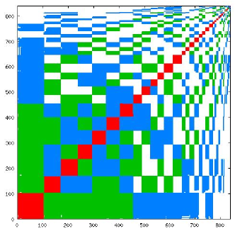
The block structure is clearly a consequence of the shell model with its subshells. It is bound to occur in every major shell. The structure is completely absent in the GOE where the matrices are densely filled. It is clear that a single matrix $C_{\mu\nu}(J,\alpha)$ cannot mix the states completely. Such mixing can be accomplished only by a linear combination of most or all of the $C_{\mu\nu}(J,\alpha)$ as in Eq. (6). Put differently, it is clear that a single or a few non–vanishing matrix elements $v(\alpha)$ cannot lead to a complete mixing of the basis states, i.e., to chaos. We expect that we need most or all of the $v(\alpha)$ for that purpose. This observation illustrates the caveat “with the exception of a set of measure zero” used in Subsection II.2: Putting one or several of the $v(\alpha)$’s identically equal to zero reduces the set $\{v(\alpha)\}$ to a set of measure zero with respect to the integration over all the variables $v(\alpha)$. The observation also sheds light on and reinforces the concept “geometric chaoticity” Zel . Indeed, the mixing is both, made possible and limited, by geometric constraints that result from the coupling of single-particle states to many-body states with good quantum numbers.

A few numbers may illustrate the way in which the matrices $C_{\mu\nu}(J,\alpha)$ fill their individual blocks. As a measure for such filling, we use the number of $C_{\mu\nu}(J,\alpha)$ which contribute on average to a given matrix element. When the partition is not changed (red blocks in Figure 13), that number is $25.2\pm 4.0$ (out of a total of 28 matrices). Within the red blocks, mixing is thus very thorough. This statement is supported by another measure (inverse participation ratios) not shown here. For the green blocks, the corresponding number is $7.2\pm 1.4$ (out of a total of 22 matrices) and for the blue blocks, $2.0\pm 0.9$ (out of a total of 13 matrices). Similar figures are obtained in the case of a single $j$–shell. The wealth of available numerical data (see, for instance, Figs. 11 and 12) shows that there is chaos for some choices of the $v(\alpha)$. This is not an accidental feature related to a particular choice of the residual interaction. Indeed, the numbers just given show that the mixing of states within each of the diagonal (red) blocks is virtually complete for almost every choice of the residual interaction. This fact ensures that a few non–diagonal matrix elements suffice to also mix different diagonal blocks very efficiently with each other. Thus, the seemingly small numbers cited for the green and blue blocks are actually quite sufficient to accomplish complete mixing of all states, even though some (white) blocks carry zero entries. As a result, we conclude from the structure of the matrices $C_{\mu\nu}(J,\alpha)$ that chaos is a generic structural property of the $sd$–shell. Since other major shells are structurally similar to the $sd$–shell, we conclude that chaos is generic in the shell model at large. We formulate this statement with one proviso: We have neglected the differences in the single–particle energies pertaining to different subshells. In realistic cases, our statement applies only if the magnitude of the matrix elements of the residual interaction is sufficiently large to mix different subshells sufficiently strongly. That is the case in practice.

While different subshells are mixed quite thoroughly and chaos is expected to prevail within every major shell, different major shells do largely retain their identity because the magnitudes of the $v(\alpha)$ are typically small compared to the spacings of major shells. This is demonstrated by experimental facts on the behavior of the neutron strength function or of spectroscopic factors which unfortunately cannot be presented and explained in the present framework.

We reiterate the remark that the strong mixing within a major shell does not preclude the existence of individual states at higher excitation energies that can be identified as distinct modes of motion of the nucleus (like the giant–dipole resonances). Deformed nuclei display collective motion like rotational bands and, in the ground–state domain, deviations from Wigner–Dyson spectral fluctuations. This last fact has been extensively discussed in the literature (see Ref. adel and references to earlier work therein). At this point, it is not clear how such features can be reconciled with the view of chaos in nuclei presented in this paper.

III.2 Information content of nuclear spectra

GOE spectra do not carry any information content. Spectral fluctuations in nuclei often agree with GOE predictions. Are such spectra void of physical information? We answer this provocative question in quantitative terms Pap3 but begin with a qualitative consideration.

The Hamiltonian (6) contains the matrix elements $v(\alpha)$ as parameters and is otherwise fixed. The number of these parameters is typically small compared with the matrix dimension. Therefore, a small number of data points (for instance, energies of levels with fixed spin $J$) suffices, in principle, to determine $H_{\mu\nu}(J)$. The Hamiltonian matrices of the levels with spins $J^{\prime}\neq J$ are governed by the ${\it same}$ set of matrix elements $v(\alpha)$ (only the matrices $C_{\mu\nu}(J^{\prime},\alpha)$ differ in form and dimension) and are, therefore, also known once the $v(\alpha)$ are determined. Hamiltonians describing other nuclei (different mass numbers) pertaining to the same major shell are likewise governed by the set $\{v(\alpha)\}$ and, thus, known too. (Again a caveat is needed: The set $\{v(\alpha)\}$ which empirically describes the data best may change with mass number). Thus, the situation is radically different from that of the GOE because the matrices $C_{\mu\nu}(J,\alpha)$ (the agents of chaos) are fixed by the shell model. A small number of parameters determines spectra of many $J$ values in many nuclei. TBRE spectra do carry information.

We turn to the quantitative question: How reliably can this information be deduced from data? To this end we cast the Hamiltonian (6) in another form. We seek a decomposition of the Hamiltonian into a sum of matrices that can be ordered with respect to their “relevance” or “importance”. The decomposition (6) is not useful for this purpose: The matrices $C_{\mu\nu}(J,\alpha)$ exhibit some degree of linear independence but a stronger metric concept is called for. For this purpose, we introduce the canonical scalar product for matrices, and switch from the matrices $C_{\mu\nu}(J,\alpha)$ to new matrices $B_{\mu\nu}(J,\alpha)$ that form an orthonormal basis set. With $d(J)$ the dimension of the Hilbert space spanned by the state vectors $|J\mu\rangle$, we define the real and symmetric overlap matrices

$$S_{\alpha\beta}(J)=d^{-1}(J)\ {\rm Trace}[C(J,\alpha)C(J,\beta)]\ .$$ (7)

These are diagonalized by orthogonal transformations ${\cal O}(J)$,

$$\{{\cal O}(J)S(J)[{\cal O}(J)]^{T}\}_{\alpha\beta}=s^{2}_{\alpha}(J)\delta_{\alpha\beta}$$ (8)

where $T$ denotes the transpose. The matrices $S_{\alpha\beta}(J)$ are positive semi-definite so that $s^{2}_{\alpha}(J)\geq 0$. The eigenvalues are arranged by decreasing magnitude, $s^{2}_{1}(J)\geq s^{2}_{2}(J)\geq\ldots\geq 0$. The real roots $s_{\alpha}(J)$ of the $s^{2}_{\alpha}(J)$’s are chosen positive or zero. If one or several eigenvalues vanish, we conclude from Eqs. (8) and (7) that there exist one or several linear combinations of the matrices $C(J,\alpha)$ that vanish identically. For the $a_{1}(J)$ non–vanishing eigenvalues $s^{2}_{\alpha}(J)$, we define

$$B_{\mu\nu}(J,\alpha)=\frac{1}{s_{\alpha}(J)}\sum_{\beta}{\cal O}_{\alpha\beta}C_{\mu\nu}(J,\beta)\ ,\ \alpha=1,\ldots,a_{1}(J)\ .$$ (9)

Except for possible degeneracies among the eigenvalues $s^{2}_{\alpha}(J)$, the matrices $B_{\mu\nu}(J,\alpha)$ are defined uniquely. By construction, these matrices are orthonormal with respect to the trace,

$$d^{-1}(J)\ {\rm Trace}[B(J,\alpha)B(J,\beta)]=\delta_{\alpha\beta}\ .$$ (10)

Written in terms of the matrices $B(J,\alpha)$, the Hamiltonian takes the form

$$H_{\mu\nu}(J)=\sum_{\alpha=1}^{a_{1}}w(J,\alpha)s_{\alpha}(J)B_{\mu\nu}(J,\alpha)\ .$$ (11)

We note that the eigenvalues $s^{2}_{\alpha}(J)$ indicate the weight and relevance of the corresponding basis matrix $B(J,\alpha)$ in the construction of the Hamiltonian (11). This weight has purely geometric origin. The dynamical weight $w(J,\alpha)$ stems from the two-body interaction and is given by

$$w(J,\alpha)=\sum_{\beta}{\cal O}_{\alpha\beta}v(\beta)\ ,\ \alpha=1,2,\ldots,a_{1}\ .$$ (12)

The $w(J,\alpha)$ have the same distribution as the $v(\alpha)$: They are Gaussian-distributed random variables with mean values zero and a common second moment. The form (11) of the Hamiltonian with the definitions (9) and (12) is completely equivalent to the original expression (6). It allows us to quantify the information content of nuclear spectra. If for some value of $J$ one or several eigenvalues $s^{2}_{\alpha}(J)$ vanish, the number $a_{1}(J)$ of variables $w(J,\alpha)$ is smaller than the number of elements $v(\alpha)$. For that value of $J$ it is then impossible to determine more than $a_{1}(J)$ linear combinations of the $v(\alpha)$ from data. We shall see that such vanishing eigenvalues always occur. Moreover, if some eigenvalues are significantly smaller than the leading ones, then Eq. (11) shows that their influence on the spectrum is small (we recall that the matrices $B(J,\alpha)$ obey Eq. (10)), and it will be difficult to deduce their values from data. We conclude that it is important to determine the eigenvalues $s^{2}_{\alpha}(J)$. That can be done without prior knowledge of the form of the residual interaction (i.e., of the values of the $v(\alpha)$) since the eigenvalues are determined by the matrices $C_{\mu\nu}(J,\alpha)$, i.e., by the shell model itself.

In Refs. Pap2 ; Pap3 , the distribution of the roots $s_{\alpha}(J)$ of the eigenvalues was given for a single $j$–shell with $j=19/2$ and for some nuclei in the $sd$–shell. All these distributions are very similar. By way of example, we reproduce in Fig. 14 the graph for the states with isospin zero in the nucleus ²⁴Mg.

Figure 14: Roots $s_{\alpha}(J)$ of the eigenvalues $s^{2}_{\alpha}(J)$ defined in Eq. (8) versus total spin $J$ for the $T=0$ states in ²⁴Mg. Taken from Ref. Pap3 .

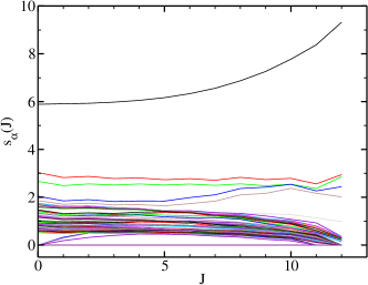
We note that all roots change smoothly with $J$. The largest, $s_{1}(J)$, is significantly larger than all others. For the case of the single $j$–shell, it can be shown analytically that the corresponding linear combination $B_{\mu\nu}(J,1)$ of the matrices $C_{\mu\nu}(J,\alpha)$ is approximately equal to the matrix representation of the monopole operator which in turn is approximately equal to the unit matrix. The numerical results indicate that these statements are generic; they hold also for ²⁴Mg. Hence, $s_{1}(J)$ determines essentially the centroid of the spectrum of states with spin $J$ and has little influence on spectral fluctuations. The latter are largely determined by the remaining non–vanishing eigenvalues and associated matrices $B_{\mu\nu}(J,\alpha)$. Because of the orthogonality relation (10), the latter are almost traceless.

The root $s_{1}(J)$ is followed in magnitude by four eigenvalues that are distinct from the remaining set. We observe that some eigenvalues in that set vanish for large values of $J$ (this is because the matrix dimension shrinks with increasing $J$ and eventually becomes too small to support a large number of eigenvalues) and that at least one eigenvalue vanishes for all values of $J$. This is because the operator ${\vec{J}}^{2}$ for total spin $J$ is a two-body operator. Thus, the matrix representation of the term ${\vec{J}}^{2}-J(J+1)$ can be written as a linear combination of the matrices $C_{\mu\nu}(J,\alpha)$. This linear combination vanishes identically.

Figure 14 shows that it is difficult to determine those $w(J,\alpha)$’s from data which belong to the smallest eigenvalues, and that the problem cannot be solved by combining data for different spin values. Practitioners of the shell model avoid the difficulty by combining a fit to data with ${\it ab\ initio}$ values of the $v(\alpha)$ obtained from many–body theory, see, for instance, Refs Bro ; Hon .

III.3 Preponderance of ground states with spin zero

In 1998, Johnson, Bertsch, and Dean Joh reported that in even–even nuclei (nuclei with even proton and neutron numbers), the TBRE yields ground states with spin zero much more frequently than corresponds to the fraction of spin-zero states in the model space. Subsequent work Bij ; Jac showed that similar regularities exist in bosonic and electronic many–body systems. The phenomenon has received intense attention, and we refer the reader to the reviews Zel1 ; Zhao1 . The problem has been understood quantitatively for bosonic models of the nucleus within mean-field calculations Bij01 . For the nuclear shell model, two approaches yield good agreement with numerical simulations. Zhao et al. Zhao2 devised an algorithm that accurately predicts the fraction of ground states with a given spin. The other approach considers fluctuations of and correlations between the $J$-dependent spectral widths and also leads to semi-quantitative predictions. It was put forward in Ref. Pap1 , and is described in what follows.

Key to the understanding of the phenomenon is the observation that the spectral widths $\sigma_{J}$ of states with different $J$ values are correlated. The spectral widths are defined by

$$\sigma^{2}_{J}=d^{-1}(J)\ {\rm Trace}[H^{2}(J)]\ .$$ (13)

From Eqs. (11) and (10), we have

$$\sigma^{2}_{J}=\sum_{\alpha=1}^{a_{1}}w^{2}(J,\alpha)s^{2}_{\alpha}(J)\ .$$ (14)

Spectral widths pertaining to different $J$ depend upon the same random variables $v(\alpha)$ (the $w(J,\alpha)$ are linear functions of the $v(\alpha)$, see Eq. (12)) and are, therefore, correlated.

Before using this fact, we relate the spectral width $\sigma_{J}$ to the position of the lowest (or highest) state with spin $J$, more precisely, to the distance $R_{J}$ of the lowest (or highest) level in the spectrum from the origin (the spectral radius). (We do not distinguish the lowest from the highest state since the $v(\alpha)$ have random signs.) The spectral radius is expected to be a random variable. We ask for the probability $p_{j}$ with which, for a given value of $J$, $R_{J}$ takes maximum value. The probability of finding a ground state with spin $J$ is given by $p_{J}$.

We define the scaling factor $r_{J}$ by writing

$$R_{J}=r_{j}\sigma_{J}\ .$$ (15)

Eq. (15) is useful in the present context because it turns out that (in contrast to $\sigma_{J}$) $r_{J}$ hardly fluctuates with the $v(\alpha)$. For the case of 6 fermions in the $j=19/2$ shell and for the states with spin $J=0$, this is shown in the inset of Fig. 15. Similarly constant (non–fluctuating) behavior of $r_{J}$ was found for other cases (different spin values, different number of nucleons, nuclei in the $sd$–shell). Therefore, the fluctuations and correlations of the widths $\sigma_{J}$ directly affect those of the spectral radii $R_{J}$. The linear fits to $r_{J}$, obtained as shown in the inset, are used for the plot of $r_{J}$ versus $J$ shown in Fig. 15 (and similarly for other cases). The overall monotonic decrease of $r_{J}$ with $J$ reflects the overall monotonic decrease of the dimensions $d(J)$ with $J$. Indeed, average shell–model spectra are known to have approximately Gaussian shape. It is then intuitively obvious that $r_{J}$ grows with $d(J)$. The decrease of $r_{J}$ with increasing $J$ shown in the figure enhances the chance for states with small spins $J$ to form the ground state. The same is true of the odd–even staggering of $r_{J}$ (which is due to the same reason and, everything else being equal, gives, for instance, preference to spin zero over spin 1).

Figure 15: (color online) The scaling factor $r_{J}$ of Eq. (15) versus $J$ for six fermions in the $j=19/2$ shell (solid line). Inset: Linear fit to $r_{J}$ for the states with $J=0$. The dots correspond to 900 realizations of the ensemble. Taken from Ref. Pap1 .

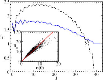
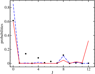
It remains to study the probabilities that the spectral widths $\sigma_{J}$ attain maximum values. For the case displayed in Fig. 15, these are shown as red lines in Fig. 16. The states with lowest and highest spins have the largest probabilities. Here the correlations play a role: For some choice of the $v(\alpha)$, the spectral width for some other spin value may take an unusually large value but so do, at the same time and for most cases, $\sigma_{0}$ and $\sigma_{42}$. The blue line in Fig. 16 gives the probability that the product $r_{J}\sigma_{J}$ attains maximum value. Because of the effect shown in Fig. 15, the highest spin value is suppressed, and spin zero wins. The result must be compared with the actual probabilities (dots) that a state with spin $J$ forms the ground state. The agreement, although not perfect, shows that the explanation accounts for the main features of the phenomenon.

Figure 16: (color online) Six fermions in the $j=19/2$ shell with 900 realizations of the TBRE. Solid red line: Numerical probabilities for $\sigma_{J}$ to have maximum value. Dashed blue line: Numerical probabilities for $r_{J}\sigma_{J}$ to have maximum value. Dots: Numerical probabilities for state with spin $J$ to be the ground state. Taken from Ref. Pap1 .

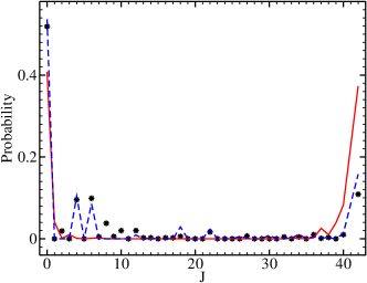
Similar results were obtained for eight Fermions in the $j=19/2$ shell, for ²⁰Ne, and for ²⁴Mg. Figure 17 shows the case of states with $T=0$ in ²⁴Mg.

Figure 17: (color online) Same as Fig. 16 for the $T=0$ states in ²⁴Mg. Taken from Ref. Pap3 .

III.4 Correlations between spectra carrying different quantum numbers

In the TBRE the preponderance of ground states with spin zero is, to a large extent, due to the correlations between spectral widths $\sigma_{J}$ pertaining to different values of $J$. The correlations are caused by the fact that all widths $\sigma_{J}$ depend on the same random variables $v(\alpha)$. Eq. (6) shows that the same statement holds for the Hamiltonians $H_{\mu\nu}(J)$ pertaining to different spin values and, more generally, for the Hamiltonians pertaining to nuclei belonging to the same major shell.

From the point of view of the shell model, these statements are not terribly surprising. A change of the residual interaction causes simultaneous changes in the spectra of all nuclei belonging to the same major shell. In the framework of a statistical description, this fact is tantamount to the existence of spectral correlations. Still, it is remarkable that such correlations have never been addressed in the framework of RMT until quite recently. It is, in fact, not obvious how to model such correlations in canonical RMT. The standard approach consists of assuming that correlations do not exist. This assumption is usually stated explicitly in the statistical theory of nuclear reactions. Let $S_{ab}(E,J)$ be an element of the statistical scattering matrix for scattering from channel $a$ into channel $b$ at energy $E$ and total spin $J$. It is assumed that elements pertaining to different $J$ values are uncorrelated. This assumption implies the symmetry of compound–nucleus scattering cross sections about $90$ degrees scattering angle in the center–of–mass system.

It is obviously of interest to test these standard assumptions of RMT using the TBRE. While tests for correlations of the statistical scattering matrix have apparently not yet been performed, tests of spectral correlations for levels both in the same nucleus carrying different quantum numbers, and in different nuclei do exist Pap3 . The level density $\rho(E,J)$ for levels with spin $J$ and energies $E_{\mu}(J)$ (where $\mu$ is a running index) is given by

$$\rho(E,J)=\sum_{\mu}\delta(E-E_{\mu}(J))\ .$$ (16)

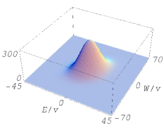
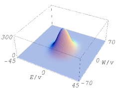
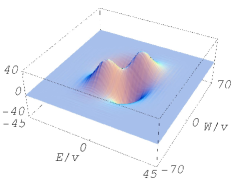
As a measure of spectral correlations, we use the correlator

$$C(E_{1},J_{1};E_{2},J_{2}) = \overline{\rho(E_{1},J_{1})\rho(E_{2},J_{2})}$$ (17)

$$\ \ -\overline{\rho(E_{1},J_{1})}\ \overline{\rho(E_{2},J_{2})}\ .$$

In Fig. 18 we show the two terms on the right–hand side of Eq. (17) and the resulting correlator versus the energies $E_{1},E_{2}$ of the two sets of spin states for the $J=0,T=0$ and the $J=2,T=0$ states in ²⁴Mg. The correlator has a maximum value of about $13$ percent of the mean value of the product of the level densities.

Figure 18: Correlations between the level densities for states with spin $0$ and spin $2$ (both with $T=0$) in ²⁴Mg. Left panel: Mean value of the product of the two level densities. Middle panel: Product of the mean level densities. Right panel: The correlator of Eq. (17). (From 400 realizations of the ensemble). Taken from Ref. Pap3 .

In Fig. 19 we show the same quantities for the $J=0,T=0$ states in ²²Ne and in ²⁴Mg. Here the correlator has a maximum value of $6$ percent. In both cases, the existence of spectral correlations is definitely established.

Figure 19: Same as Fig. 18 except for the correlations between the level densities for states with spin $0$ and isospin $0$ in ²⁰Ne and in ²⁴Mg. Left panel: Mean value of the product of the two level densities. Middle panel: Product of the mean level densities. Right panel: The correlator of Eq. (17). (From 400 realizations of the ensemble). Taken from Ref. Pap3 .

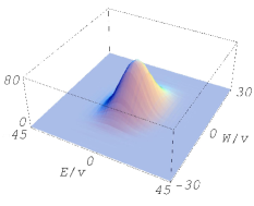
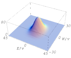
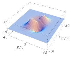
The correlators shown in Figures 18 and 19 are obtained by averaging over the ensemble and are, therefore, entirely theoretical. Do they have any correspondence in reality (where we deal with a single Hamiltonian rather than an ensemble)? Presently, this question cannot be answered using experimental data – the data set is not sufficient. However, shell–model calculations can serve as a substitute. Realistic single–particle energies and an optimized two–body interaction (the “Brown–Wildenthal interaction” Bro ) were used to calculate the energies of low–lying states with spins $J=0$ and $J=2$ ($J=1/2$ and $J=5/2$) in a number of even–even (odd–even, respectively) nuclei in the $sd$–shell Pap3 . The correlations between nearest–neighbor level spacings of the lowest few states with different spins were evaluated as in Eq. (17), the ensemble average being replaced by the running average over the set of nuclei just mentioned. Figure 20 shows the result (displayed in the same form as in Figs. 18 and 19). Again, the existence of correlations is established. We observe that these are particularly pronounced for the lowest levels where they amount to about $10$ percent.

Figure 20: Same as Fig. 18 except for the correlations between pairs of nearest–neighbor spacings of low–lying levels with different spins obtained by averaging over a number of nuclei in the $sd$–shell (see text). The indices $i$ and $j$ label the spacings consecutively starting from the lowest state. Left panel: Mean value of the product of the two spacings. Middle panel: Product of the mean values of the two spacings. Right panel: The correlator. Taken from Ref. Pap3 .

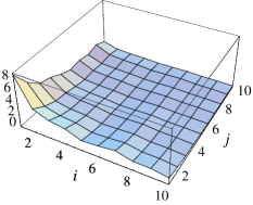
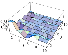
Our analysis establishes the existence of correlations between spectra carrying different quantum numbers. All examples were taken from the $sd$–shell, however, where the dimensions of the Hamiltonian matrices are rather small (typically $10^{2}$ to $10^{3}$). The maxima of the correlators are in the $10$ percent range. It is not clear how these results carry over to other major shells where both the matrix dimensions and the number of independent two–body matrix elements are much bigger. The statistical theory of nuclear reactions is mainly used in such shells. Therefore, definitive conclusions must wait for a further analysis.

IV Summary and Conclusions

In the first part of this paper, we have introduced random matrices and the concept of (quantum) chaos. Both are linked by the Bohigas–Giannoni–Schmit conjecture. Random–matrix theory predicts fluctuation properties of spectra in a parameter–free fashion. In many cases, the fluctuation properties of nuclear spectra agree with these predictions: The nuclear dynamics is (partly) chaotic. To relate this observation to known dynamical features of spherical nuclei, we have, in the second part, described the nuclear shell model (a mean–field theory with residual interactions). We have pointed out that shell–model spectra also show chaos. To explain this observation, we have defined the two–body random ensemble (TBRE) as the generic Gaussian random–matrix ensemble of the shell model. In part three, we have displayed a number of properties of that ensemble, mainly using the $sd$–shell. We have focused attention on those properties in which the TBRE differs from standard RMT: (i) The TBRE generically produces chaos. Thus, chaos in nuclei is not due to a particular feature of the residual interaction. The mechanism which mixes the basis states of Hilbert space differs significantly from that of canonical RMT. Chaos is due to the “building block” matrices $C_{\mu\nu}(J,\alpha)$. In each major shell, these matrices are fixed once and for all. They are determined entirely by intrinsic properties of the shell model and are independent of any particular residual interaction. (ii) The spectra of matrices drawn at random from a canonical ensemble of RMT do not carry any information content. Because of the role played by the fixed matrices $C_{\mu\nu}(J,\alpha)$, this is not so for the TBRE. On the contrary, it is possible to extract relevant physical information from nuclear spectra. We have analyzed the degree to which this can be done. (iii) The preponderance of ground states with spin zero in the TBRE is, to a large extent, due to correlations between widths of spectra with different spin values. (iv) Correlations exist more generally also between spectra carrying different quantum numbers and in different nuclei belonging to the same major shell. The implications of this last statement have not yet been fully explored.

The examples used to illustrate or prove these assertions were taken from the $sd$–shell or from a single $j$–shell. The line of reasoning suggests very strongly, however, that the spectral fluctuation properties of the TBRE agree with RMT predictions for all major shells. We have confined ourselves to a two–body residual interaction and to the TBRE. It is obvious that the inclusion of three–body forces would enhance the tendency of the system towards chaotic dynamics.

Throughout most of the paper, we have assumed that the single–particle energies of subshells belonging to a major shell are degenerate. Within this approximation, we have shown that quantum chaos is a generic feature of the nuclear shell model. This means that most choices of the residual interaction (but not all) will result in spectra showing spectral fluctuations that agree with RMT predictions. Actually, the neglect of the differences of single–particle energies of subshells is not completely justified. The magnitude of a typical two–body matrix element which mixes different subshells is comparable with the difference of the corresponding single–particle energies. The resulting incomplete mixing of many–body states within a major shell reveals itself in slight deviations from RMT predictions Zel . Moreover, the residual interaction is far too weak to thoroughly mix adjacent major shells. This is why shell structure remains the hallmark of nuclear physics, in spite of quantum chaos. It is in that sense that spherical nuclei display only partial quantum chaos.

Low–lying states in spherical nuclei often display regular features. This statement is not at variance with our conclusions. Indeed, chaos manifests itself mainly in the fluctuation properties of spectra. These are defined in terms of statistical measures tests of which require a large number of levels with identical quantum numbers. The regular features just mentioned refer to properties of a small number of levels in the ground–state domain which carry different quantum numbers. The properties of these levels may be particularly sensitive to a specific component of the two–body interaction. Modelling the entire residual interaction in terms of that component may give rise to regular motion.

Our discussion has been confined to spherical nuclei. Nuclei with mass numbers lying in the middle of large major shells (like the rare–earth nuclei) cannot be successfully described in terms of the spherical shell model. The dimensions of the many–body Hilbert spaces are too large. One uses instead collective models with a small number of degrees of freedom. The connection between these and the spherical shell model is not firmly established. However, quantum chaos is prevalent in these nuclei, too, with the exception of cases of distinct symmetries Whe .

There are several open questions and directions for future research. (i) We are still lacking a deeper analytical understanding of the TBRE and its fluctuation properties. An analytical approach must be based on properties of the matrices denoted by $C_{\mu\nu}(J,\alpha)$ in this paper. While a theoretical description for shells with several subshells is probably very difficult, focus on a single $j$–shell might simplify the problem. (ii) The TBRE predicts correlations between spectra with different quantum numbers (e.g., different masses, spins, or isospins) for nuclei within a major shell. The expermimental verification is difficult due to limitations in the length and completeness of observed nuclear spectra, but other Fermi systems might be more accessible. (iii) The correlations between spectra with different quantum numbers might also affect the scattering matrix, more precisely: Such correlations might induce correlations among $S$–matrix elements carrying different total spin quantum numbers. The present analysis of fluctuating cross sections in compound nuclei neglects any such correlations. A better understanding of this problem would be highly desirable.

Nuclear spectroscopy is a mature field with a history of more than 50 years. In spite of this fact it continues to offer great challenges. We have addressed one of them: The way chaos is induced by the two–body interaction of the shell model, an interaction which is at the same time responsible for the many regular features seen in nuclei.