Temperature-dependent errors in nuclear lattice simulations

Abstract

We study the temperature dependence of discretization errors in nuclear lattice simulations.  We find that for systems with strong attractive interactions the predominant error arises from the breaking of Galilean invariance.  We propose a local “well-tempered” lattice action which eliminates much of this error.  The well-tempered action can be readily implemented in lattice simulations for nuclear systems as well as cold atomic Fermi systems.

I Introduction

Nuclear lattice simulations address the nuclear many-body problem by combining numerical lattice methods with effective field theory.  There have been several recent studies on the subject of nuclear lattice simulations Müller et al. (2000); Abe et al. (2004); Lee et al. (2004); Lee and Schaefer (2005); Hamilton et al. (2005); Seki and van Kolck (2006); Lee and Schafer (2006a, b); Borasoy et al. (2006a, b).  The starting point is the usual starting point of effective field theory.  All local interactions consistent with the symmetries of low-energy nuclear physics are organized by counting factors of $Q/\Lambda_{\text{high}}$, where$\ Q$ is the typical nucleon momentum scale and $\Lambda_{\text{high}}$ is the high-momentum scale where the effective theory eventually breaks down.  For chiral effective field theory we have $\Lambda_{\text{high}}\sim 4\pi f_{\pi},$ and for effective field theory without pions $\Lambda_{\text{high}}\sim m_{\pi}$.  Interactions in the effective theory are truncated at some order in $Q/\Lambda_{\text{high}}$, and the remaining interactions are put on a space-time lattice.  Coefficients for the interactions are determined by matching to scattering phase shifts and few-nucleon spectra.  Once the interaction coefficients of the lattice effective theory are determined, the many-body system can be simulated nonperturbatively using Monte Carlo.  The method can be applied to nuclei at zero temperature as well as the thermodynamics of nuclear and neutron matter at nonzero temperature.  Similar lattice effective field theory techniques have been used to study cold atomic Fermi systems in the limit of short range interactions and long scattering length Chen and Kaplan (2004); Wingate (2005); Bulgac et al. (2006); Lee (2006); Burovski et al. (2006a, b); Lee .

In addition to $Q$ and $\Lambda_{\text{high}}$ there is also a momentum cutoff scale $\Lambda$.  On the lattice with lattice spacing $a$, the cutoff momentum scale is $\Lambda=\pi a^{-1}$.  Ideally one should increase $\Lambda$ systematically to extrapolate to the continuum limit $\Lambda\rightarrow\infty$.  For any finite set of diagrams with the required local counterterms this is not a problem.  However when diagrams are iterated to all orders complications arise when the interactions involve singular potentials.  For example in pionless effective field theory it is known that a three-body counterterm is required at leading order Efimov (1971, 1993); Bedaque et al. (1999a, b); Bedaque et al. (2000); Platter et al. (2004, 2005); Braaten and Hammer (2006); Borasoy et al. (2006a); Platter (2006).  With the three-body counterterm in place the continuum limit is well defined for few-body calculations.  Unfortunately at very high cutoff momentum this approach involves removing spurious deeply-bound states by hand, and there is no way to do this in many-body simulations.  The problem is no better in effective field theory with pions.  In this case the pion tensor force generates instabilities in higher partial wave channels at large $\Lambda$ Nogga et al. (2005); Birse (2005); Epelbaum (2006); Epelbaum and Meißner (2006).  In short the presence of continuum limit instabilities and computational constraints means that for many-body simulations one is restricted to a finite range of values for $\Lambda$.  Therefore it is important to understand and control errors that occur at finite cutoff momentum.

In this study we investigate finite cutoff errors on the lattice at nonzero temperature.  While our results and conclusions apply to general few- and many-body nuclear systems, we center our discussion on simulations of dilute neutron matter.  In particular we consider an idealized limit of neutron matter with zero range two-body interactions.  We take this zero-range two-body contact interaction as the only interaction.  Therefore $\Lambda_{\text{high}}\rightarrow\infty,$ and it is straightforward to show that this idealized theory has no continuum limit instabilities.  For these reasons it is a useful testing ground to study $Q/\Lambda$ cutoff errors without additional complications.  Zero-range neutron matter is a good approximation to actual dilute neutron matter when the spacing between neutrons is sufficiently large.  This occurs at about $1\%$ of normal nuclear matter density or less.

Our interest in finite cutoff errors at nonzero temperature is motivated by a recent analysis of zero-range neutron matter on the lattice which found sizable lattice errors at nonzero temperature Lee and Schafer (2006a).  This stands in contrast with zero temperature simulations which found little dependence on lattice spacing Lee (2006, ).  The lattice spacing dependence at nonzero temperature was first noticed in the results of many-body lattice simulations and then analyzed by calculating coefficients of the virial expansion.  The second-order virial coefficient $b_{2}(T)$, where $T$ is temperature, was found to be too large when computed on the lattice.  While the source of the error was unknown, it was suggested that tuning the two-body interaction to give the correct value for $b_{2}(T)$ might improve the results of the many-body simulation.  This suggestion was carried out in Lee and Schafer (2006b), and the many-body lattice results with the retuned interaction showed little residual dependence on lattice spacing.  Similar cutoff errors were found in Burovski et al. (2006a, b).  However the analysis did not distinguish between cutoff errors due to nonzero temperature and cutoff errors due to nonzero density.

In this paper we answer some of the questions raised by the findings in Lee and Schafer (2006a) and Lee and Schafer (2006b).  In particular we discuss the source of the large temperature-dependent lattice errors, why the measured energies tended to be too low, and why in Lee and Schafer (2006b) it was possible to cancel much of the error by retuning the two-body interaction.  We also propose a simple modified lattice action which eliminates most of the large temperature-dependent lattice errors from the beginning.  The results of our analysis should be useful for reducing systematic errors in future nuclear lattice simulations as well as other strongly-attractive fermionic systems.

II Virial expansion

The virial expansion for the equation of state has been used to study neutron and nuclear matter as well as fermionic atoms near the classical regime Ho and Mueller (2004); Horowitz and Schwenk (2005a, b); Rupak (2006)  The virial expansion can be regarded as a power series in fugacity, $z=e^{\beta\mu}$, where $\beta$ is the inverse temperature and $\mu$ is the chemical potential.  For example the logarithm of the grand canonical partition function per unit volume for neutron matter can be written as

$$\frac{1}{V}\ln Z_{G}=\frac{2}{\lambda_{T}^{3}}\left[z+b_{2}(T)z^{2}+b_{3}(T)z^{3}\cdots\right],$$ (1)

where

$$\lambda_{T}=\sqrt{\frac{2\pi\beta}{m}}$$ (2)

is the thermal wavelength and $m$ is the neutron mass.  We can use the virial expansion to compute thermodynamic observables when the thermal wavelength is smaller than the interparticle spacing.  The neutron density, $\rho$, can be computed by taking a derivative of $\ln Z_{G}$ with respect to the chemical potential,

$$\rho=\frac{1}{\beta V}\frac{\partial}{\partial\mu}\ln Z_{G}\text{.}$$ (3)

To second order in the virial expansion we find

$$\rho=\frac{2}{\lambda_{T}^{3}}\left[z+2b_{2}(T)z^{2}+\cdots\right].$$ (4)

Taking into account Fermi statistics, we get

$$b_{2}^{\text{free}}(T)=-2^{-5/2}\approx-0.177$$ (5)

for a free gas of neutrons.

With the interactions turned on, the second virial coefficient can be computed by extracting the term in the partition function proportional to $z^{2}$,

$$b_{2}(T)-b_{2}^{\text{free}}(T)=\frac{\lambda_{T}^{3}}{2V}\left\{Tr_{2}[\text{exp}(-\beta H)]-Tr_{2}[\text{exp}(-\beta H_{\text{free}})]\right\}.$$ (6)

$Tr_{2}$ denotes the trace over all two neutron states, $H$ is the full Hamiltonian, and $H_{\text{free}}$ is the free Hamiltonian.  By integrating over the center of mass momentum and enforcing spherical boundary conditions on the relative displacement between the two particles, the density of scattering states can be related to the total elastic phase shift $\delta(E)$ Beth and Uhlenbeck (1937),

$$b_{2}(T)-b_{2}^{\text{free}}(T)=\frac{\beta}{2^{1/2}\pi}\int_{0}^{\infty}dE\;e^{-\beta E/2}\delta(E)+\text{bound state contribution.}$$ (7)

If there are two-body bound states in the spectrum with binding energies $E_{B,i}$, there is an additional contribution

$$\frac{3}{2^{1/2}}{\displaystyle\sum\limits_{i}}\left(e^{\beta\left|E_{B,i}\right|}-1\right).$$ (8)

In the unitary limit, where the effective range is zero and scattering length is infinite, we get

$$b_{2}(T)=3\times 2^{-\frac{5}{2}}\approx 0.530.$$ (9)

For zero effective range but arbitrary scattering length $a_{\text{scatt}}$ the second virial coefficient is

$$b_{2}(T)=\left\{\genfrac{}{}{0.0pt}{}{\frac{e^{x^{2}}}{\sqrt{2}}\left[1-\operatorname{erf}(\left|x\right|)\right]-\frac{1}{4\sqrt{2}}\text{ \ for }x<0,}{\sqrt{2}e^{\frac{\left|E_{B}\right|}{k_{B}T}}-\frac{e^{x^{2}}}{\sqrt{2}}\left[1-\operatorname{erf}(x)\right]-\frac{1}{4\sqrt{2}}\text{ \ for }x>0,}\right.$$ (10)

where $\operatorname{erf}$ is the error function, $E_{B}$ is the two-particle binding energy for positive scattering length, and

$$x=\frac{\lambda_{T}}{\sqrt{2\pi}a_{\text{scatt}}}.$$ (11)

As the effective range goes to zero we have the relation

$$\left|E_{B}\right|=\frac{1}{ma_{\text{scatt}}^{2}},$$ (12)

and therefore we can write

$$b_{2}(T)=\left\{\genfrac{}{}{0.0pt}{}{\frac{e^{x^{2}}}{\sqrt{2}}\left[1-\operatorname{erf}(\left|x\right|)\right]-\frac{1}{4\sqrt{2}}\text{ \ for }x<0,}{\frac{e^{x^{2}}}{\sqrt{2}}\left[1+\operatorname{erf}(x)\right]-\frac{1}{4\sqrt{2}}\text{ \ for }x>0.}\right.$$ (13)

III One-dimensional model

We begin our analysis of finite cutoff errors with a one-dimensional model.  The model consists of nonrelativistic spin-1/2 fermions with an attractive zero-range interaction and is the continuum limit of the attractive one-dimensional Hubbard model.  Both the attractive and repulsive versions of the one-dimensional Hubbard model have been studied in the literature Yang (1967); Lieb and Wu (1968); McGuire (1966); Ahn et al. (1995); Matveenko (1998); Guerrero et al. ; Salwen et al. (2004).  We consider the attractive case as a toy model of short-range attractive forces in nuclear systems.  As we will see, the problem of large discretization errors appears even in this one-dimensional model which has no ultraviolet divergences.

In the continuum limit the Hamiltonian has the form

$$H=-\frac{1}{2m}\sum_{i=\uparrow,\downarrow}\int dx\;a_{i}^{\dagger}(x)\frac{\partial^{2}}{\partial x^{2}}a_{i}(x)+C\int dx\;a_{\downarrow}^{\dagger}(x)a_{\uparrow}^{\dagger}(x)a_{\uparrow}(x)a_{\downarrow}(x),$$ (14)

where $m$ is the mass, $C<0$, and $a_{i}$ and $a_{i}^{\dagger}$ are annihilation and creation operators for spin $i$.  The connected amputated two-particle Green’s function equals the sum of bubble diagrams shown in Fig. 1.

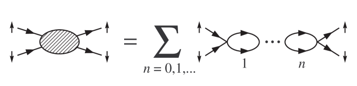
Figure 1: The connected amputated two-particle Green’s function.

Any connected scattering process consists of two-particle Green’s functions linked together with free particle propagators.

Let $G_{2}(p_{0},p_{x})$ be the amplitude for the connected amputated two-particle Green’s function, where$\ p_{0}$ is the total energy and $p_{x}$ is the total spatial momentum of the two particles.  We sum the bubble diagrams in Fig. 1 and get

$$G_{2}(p_{0},p_{x})=\frac{-iC}{1-iC\cdot\Pi\left(p_{0},p_{x}\right)}=\frac{1}{-\frac{1}{iC}+\Pi\left(p_{0},p_{x}\right)},$$ (15)

where

$$\Pi\left(p_{0},p_{x}\right)=\int\frac{dq_{0}dq_{x}}{\left(2\pi\right)^{2}}\frac{i}{\frac{p_{0}}{2}+q_{0}-\frac{\left(\frac{p_{x}}{2}+q_{x}\right)^{2}}{2m}+i\varepsilon}\times\frac{i}{\frac{p_{0}}{2}-q_{0}-\frac{\left(\frac{p_{x}}{2}-q_{x}\right)^{2}}{2m}+i\varepsilon}.$$ (16)

In the continuum limit we find

$$\Pi\left(p_{0},p_{x}\right) =-\frac{m}{2\sqrt{mp_{0}-\frac{p_{x}^{2}}{4}}},$$ (17)

$$G_{2}(p_{0},p_{x}) =\frac{1}{-\frac{1}{iC}-\frac{m}{2\sqrt{mp_{0}-\frac{p_{x}^{2}}{4}}}}.$$ (18)

Since $C<0$ there is a bound state pole in the two-particle Green’s function at energy

$$p_{0}=-\frac{mC^{2}}{4}+\frac{p_{x}^{2}}{4m}.$$ (19)

We can obtain the same result by solving the Schrödinger equation for the two-particle system in the center of mass frame.  If $x$ is the relative separation between particles then, in the center of mass frame, the reduced Hamiltonian is

$$H_{CM}=-\frac{1}{m}\frac{\partial^{2}}{\partial x^{2}}+C\delta(x),$$ (20)

and the ground state wavefunction is

$$\psi_{0}(x)\propto\exp\left(\frac{1}{2}mC\left|x\right|\right).$$ (21)

The ground state energy with center of mass kinetic energy included is

$$E_{0}(p_{x})=-\frac{mC^{2}}{4}+\frac{p_{x}^{2}}{4m},$$ (22)

where $p_{x}$ is the total momentum.

The one-dimensional system is finite in the continuum limit and therefore no regularization nor renormalization is needed.  Nevertheless we impose an ultraviolet cutoff on the momentum in order to study the resulting cutoff errors.   With a momentum cutoff at $\Lambda$ we find

$$\Pi\left(p_{0},p_{x},\Lambda\right)=-\frac{m}{2\sqrt{mp_{0}-\frac{p_{x}^{2}}{4}}}\times\left[1+O\left(\frac{Q^{2}}{\Lambda^{2}}\right)\right],$$ (23)

where $Q^{2}$ is some homogeneous combination of the parameters $mp_{0}$ and $p_{x}^{2}$.  The combination will depend on the details of the chosen regularization scheme.  The regularized two-particle Green’s function has the form

$$G_{2}(p_{0},p_{x},\Lambda)=\frac{1}{-\frac{1}{iC(\Lambda)}-\frac{m}{2\sqrt{mp_{0}-\frac{p_{x}^{2}}{4}}}\times\left[1+O\left(\frac{Q^{2}}{\Lambda^{2}}\right)\right]}.$$ (24)

We define the scale-dependent coupling $C(\Lambda)$ so that the pole in the rest frame remains exactly at

$$p_{0}=-\frac{mC^{2}}{4}.$$ (25)

III.1 One- and two-particle lattice dispersion relation in one dimension

We investigate the cutoff error in more detail using a Hamiltonian lattice formalism.  On the lattice the cutoff momentum scale $\Lambda$ corresponds with $\pi a^{-1}$, where $a$ is the lattice spacing.  Throughout our discussion of the lattice formalism we use dimensionless parameters and operators, which correspond with physical values multiplied by the appropriate power of $a$.  However final results are reported into physical units.  We start with the simplest possible lattice Hamiltonian giving (14) in the continuum limit.  We let

$$H^{(0)}=K^{(0)}+V^{(0)},$$ (26)

$$K^{(0)}=\frac{1}{m}\sum_{n_{x},i}a_{i}^{\dagger}(n_{x})a_{i}(n_{x})-\frac{1}{2m}\sum_{n_{x},i}\left[a_{i}^{\dagger}(n_{x})a_{i}(n_{x}+1)+a_{i}^{\dagger}(n_{x})a_{i}(n_{x}-1)\right],$$ (27)

$$V^{(0)}=C\sum_{n_{x}}a_{\downarrow}^{\dagger}(n_{x})a_{\uparrow}^{\dagger}(n_{x})a_{\uparrow}(n_{x})a_{\downarrow}(n_{x}).$$ (28)

We refer to $H^{(0)}$ as the standard lattice Hamiltonian.  The zero superscript signifies that it is the simplest possible lattice formulation.  Later in our discussion we consider more complicated lattice actions.  We choose the mass to be $m=939$ MeV and fix the lattice spacing at $a=(50$ MeV$)^{-1}$.  This corresponds with a cutoff momentum of $\Lambda=\pi a^{-1}\simeq 157$ MeV.

The single-particle dispersion relation for the standard lattice Hamiltonian is given by

$$\omega^{(0)}(p_{x})=\frac{1}{m}\times\left(1-\cos p_{x}\right)=\frac{p_{x}^{2}}{2m}+O\left(p_{x}^{4}\right).$$ (29)

In Fig. 2 we have plotted $\omega^{(0)}(p_{x})$ versus the continuum result $\omega(p_{x})=p_{x}^{2}/(2m)$ for momenta in the first Brillouin zone $\left|p_{x}\right|\leq\Lambda$.

Figure 2: Single-particle dispersion relation for the standard lattice action with $m=939$ MeV and $\Lambda=\pi a^{-1}\simeq 157$ MeV.  We also show the continuum limit.

The relative error between $\omega^{(0)}$ and $\omega$ is $10\%$ or less for $\left|p_{x}\right|<\Lambda/3.$

We now consider two-particle states with one spin-up particle and one spin-down particle.  We start with a small value for the coupling, $C=-0.0400$.  Let $p_{x}$ be the total momentum of the two-particle system.  In the continuum limit the ground state energy at zero total momentum is

$$E_{0}(p_{x}=0)=-\frac{mC^{2}}{4}=-0.3756\text{\ MeV.}$$ (30)

It is convenient to place the two-particle system in a periodic box.  We choose the box length to be $L=1$ MeV^-1.  Since the ground state wavefunction depends on the relative separation $x$ as

$$\psi_{0}(x)\propto\exp\left(\frac{1}{2}mC\left|x\right|\right)\approx\exp\left[-(19\text{\ MeV)}\cdot\left|x\right|\right],$$ (31)

the effect of the boundary at $L=1$ MeV^-1 on the ground state energy is negligible.  The box length does however determine the level spacing between unbound scattering states.

For the lattice calculation the interaction strength is tuned so that the ground state energy in the rest frame matches the continuum result of $-0.3756$ MeV.  This gives an adjusted coefficient of $C(\Lambda)\simeq-0.0407.$  In Fig. 3 we show the two lowest energy levels of the two-particle system as functions of $p_{x}$.  The two-particle ground state and lowest scattering state energies for the lattice are labelled $E_{0}^{(0)}$ and $E_{1}^{(0)}$ respectively, while the corresponding continuum limit values are labelled $E_{0}$ and $E_{1}$.

Figure 3: The lowest two-particle energies for the standard lattice action, $E_{0}^{(0)}$ and $E_{1}^{(0)}$, and the corresponding continuum limit values, $E_{0}$ and $E_{1}$.  The continuum coupling is $C=-0.0400$ while the lattice coupling is $C(\Lambda)=-0.0407.$

The mismatch between lattice and continuum results for the two-particle energies is roughly the same size as the mismatch between single-particle lattice and continuum kinetic energies, $\omega^{(0)}$ and $\omega$.

Keeping other parameters the same we now repeat the two-particle energy calculations at stronger coupling, $C=-0.1000$.  In this case the continuum limit ground state energy at $p_{x}=0$ is

$$E_{0}(p_{x}=0)=-\frac{mC^{2}}{4}=-2.348\text{\ MeV.}$$ (32)

Tuning the lattice interaction to match this ground state energy gives an adjusted coefficient of $C(\Lambda)\simeq-0.1105$.  Results for the two-particle ground state and lowest scattering state are shown in Fig. 4.

Figure 4: The lowest two-particle energies for the standard lattice action, $E_{0}^{(0)}$ and $E_{1}^{(0)}$, and the corresponding continuum limit values, $E_{0}$ and $E_{1}$.  The continuum coupling is $C=-0.1000$ while the lattice coupling is $C(\Lambda)=-0.1105.$

While the agreement for the first excited states $E_{1}^{(0)}$ and $E_{1}$ has not changed noticeably, the deviation between lattice and continuum results for the ground state energy has increased substantially for $p_{x}\neq 0$.  We have chosen the lattice coupling $C(\Lambda)$ so that $E_{0}^{(0)}=E_{0}$ at $p_{x}=0,$ and so the disagreement between $E_{0}^{(0)}$ and $E_{0}$ is proportional $p_{x}^{2}.$

III.2 Broken Galilean invariance

In the continuum limit Galilean invariance requires that the total energy of the two-particle system rises quadratically with the total momentum $p_{x}$,

$$E(p_{x})=E(0)+\frac{p_{x}^{2}}{4m}.$$ (33)

However any regularization scheme with a preferred reference frame breaks Galilean invariance to some extent.  In the following we show how broken Galilean invariance on the lattice can result in large cutoff errors at strong coupling.

Let the momenta of the two particles be $p_{x}/2-q_{x}$ and $p_{x}/2+q_{x}$, where $p_{x}$ is the total momentum and $2q_{x}$ is the relative momentum between the particles.  We consider first the ground state.  The average value of the relative momentum $2q_{x}$ for the two-body ground state wavefunction grows proportionally with $m\left|C\right|$.  For $C=-0.0400$ we have $m\left|C\right|=37.6$ MeV, while for $C=-0.1000$ we have $m\left|C\right|=93.9$ MeV.  For the latter case $2q_{x}$ is not small compared with the cutoff momentum $157$ MeV.  It is not so large as to invalidate the assumption that we have a sensible low-energy effective field theory.  However it is large enough that one of the constituent particle momenta can reach the Brillouin zone boundary at $\pm\Lambda$ even though $\left|p_{x}/2\right|$ is less than $\Lambda$.  At the zone boundary the lattice kinetic energy $\omega^{(0)}$ is significantly lower than the continuum kinetic energy $\omega$.  This error in the dispersion relation produces a ground state energy $E_{0}^{(0)}(p_{x})$ which is lower than the continuum result $E_{0}(p_{x})$ at strong coupling.  This is the effect we observe in Fig. 4.

The problem with large relative momentum does not occur for low-energy scattering states above the ground state.  This is because the wavefunctions for these scattering states are peaked around the asymptotic momenta of the particles, $p_{x}/2-q_{x}$ and $p_{x}/2+q_{x}$.  In the infinite $L$ limit we have

$$E=\frac{1}{2m}\left(\frac{p_{x}}{2}-q_{x}\right)^{2}+\frac{1}{2m}\left(\frac{p_{x}}{2}+q_{x}\right)^{2}=\frac{p_{x}^{2}}{4m}+\frac{q_{x}^{2}}{m},$$ (34)

$$q_{x}^{2}=mE-\frac{p_{x}^{2}}{4}.$$ (35)

If $mE$ and $p_{x}^{2}$ are much less than $\Lambda^{2}$, it follows that $q_{x}^{2}$ is also much less than $\Lambda^{2}$.  Hence the single-particle momenta $p_{x}/2-q_{x}$ and $p_{x}/2+q_{x}$ are small compared with $\Lambda,$ and cutoff errors should remain small for low-energy scattering states even at strong coupling.

III.3 Cutoff errors at nonzero temperature

In the classical regime the equipartition theorem tells us that the distribution of momenta $p_{x}$ satisfies

$$\left\langle\frac{p_{x}^{2}}{4m}\right\rangle=\frac{1}{2}T,\qquad p_{x}^{\text{rms}}=\sqrt{2mT}.$$ (36)

Since the cutoff errors are proportional to $p_{x}^{2}$, this suggests that at fixed lattice spacing the cutoff errors for the dilute system should increase linearly with $T$.  One approach to removing this error at nonzero $T$ is to define the lattice coupling $C(\Lambda)$ by matching the continuum energy $E_{0}(p_{x})$ at $\left|p_{x}\right|=\sqrt{2mT}$ rather than at $p_{x}=0.$  In Fig. 5 we show the two-particle energies when $C(\Lambda)$ is fit to $E_{0}(p_{x})$ at $\left|p_{x}\right|=p_{x}^{\text{rms}}\simeq 60$ MeV.

Figure 5: The two-particle energies for the lattice, $E_{0}^{(0)}$ and $E_{1}^{(0)}$, and continuum, $E_{0}$ and $E_{1}$. The continuum coupling is $C=-0.1000$ while the lattice coupling $C(\Lambda)$ is set by matching $E_{0}(p_{x})$ at $\left|p_{x}\right|=p_{x}^{\text{rms}}\simeq 60$ MeV.

This redefinition has the unattractive feature that the lattice coupling $C(\Lambda)$ is now temperature dependent.  Furthermore it does not fix the problem of strongly-broken Galilean invariance.  The cutoff error has simply been shifted to momenta $\left|p_{x}\right|\neq p_{x}^{\text{rms}}$.  However it does remove large cutoff errors from the lattice simulation at temperature $T$.  This is essentially the approach used in Lee and Schafer (2006a, b), where the lattice coupling $C(\Lambda)$ was determined by matching the continuum limit value for the second virial coefficient $b_{2}(T)$, where $T$ is the chosen simulation temperature.

There are other techniques which actually reduce the breaking of Galilean invariance on the lattice.  One possibility is to remove all of the $O\left(\frac{Q^{2}}{\Lambda^{2}}\right)$ dependence using higher-dimensional operators.  This includes two-derivative interactions such as

$$O_{1}(x)=\frac{d}{dx}\left[a_{\downarrow}^{\dagger}(x)a_{\uparrow}^{\dagger}(x)\right]\frac{d}{dx}\left[a_{\uparrow}(x)a_{\downarrow}(x)\right],$$ (37)

$$O_{2}(x) =a_{\downarrow}^{\dagger}(x)a_{\uparrow}^{\dagger}(x)\left[\frac{d^{2}a_{\uparrow}(x)}{dx^{2}}a_{\downarrow}(x)-2\frac{da_{\uparrow}(x)}{dx}\frac{da_{\downarrow}(x)}{dx}+a_{\uparrow}(x)\frac{d^{2}a_{\downarrow}(x)}{dx^{2}}\right]$$

$$+\left[\frac{d^{2}a_{\downarrow}^{\dagger}(x)}{dx^{2}}a_{\uparrow}^{\dagger}(x)-2\frac{da_{\downarrow}^{\dagger}(x)}{dx}\frac{da_{\uparrow}^{\dagger}(x)}{dx}+a_{\downarrow}^{\dagger}(x)\frac{d^{2}a_{\uparrow}^{\dagger}(x)}{dx^{2}}\right]a_{\uparrow}(x)a_{\downarrow}(x).$$ (38)

$O_{1}$ could be tuned to cancel the broken Galilean invariance while $O_{2}$ could be tuned to reset the effective range to zero.  However new interactions such as these can introduce sign oscillations and other complications in Monte Carlo simulations.  Therefore we first try a less expensive approach where the interaction is left alone and only the lattice kinetic energy is modified.

III.4 $O(a^{2})$-improved and $O(a^{2})$-well-tempered actions in one dimension

Let us consider replacing the standard lattice kinetic energy action in (27) with an $O(a^{2})$-improved kinetic energy with next-to-nearest neighbor hopping,

$$K^{(1)} =\frac{5}{4}\times\frac{1}{m}\sum_{n_{x},i}a_{i}^{\dagger}(n_{x})a_{i}(n_{x})-\frac{4}{3}\times\frac{1}{2m}\sum_{n_{x},i}\left[a_{i}^{\dagger}(n_{x})a_{i}(n_{x}+1)+a_{i}^{\dagger}(n_{x})a_{i}(n_{x}-1)\right]$$

$$+\frac{1}{12}\times\frac{1}{2m}\sum_{n_{x},i}\left[a_{i}^{\dagger}(n_{x})a_{i}(n_{x}+2)+a_{i}^{\dagger}(n_{x})a_{i}(n_{x}-2)\right].$$ (39)

This gives the dispersion relation

$$\omega^{(1)}(p_{x})=\frac{1}{m}\times\left[\frac{5}{4}-\frac{4}{3}\cos p_{x}+\frac{1}{12}\cos\left(2p_{x}\right)\right]=\frac{p_{x}^{2}}{2m}+O\left(p_{x}^{6}\right).$$ (40)

Matching $E_{0}(p_{x}=0)=-2.348$ MeV for the improved lattice action gives an adjusted coefficient of $C(\Lambda)=-0.1173$.  Results for the two-particle ground state and lowest scattering state with the improved action are shown in Fig. 6.

Figure 6: The lowest two-particle energies for the improved lattice action, $E_{0}^{(1)}$ and $E_{1}^{(1)}$, and the continuum energies, $E_{0}$ and $E_{1}$.  The continuum coupling is $C=-0.1000$ while the lattice coupling is $C(\Lambda)=-0.1173$.

We see that the deviation between lattice and continuum results for the ground state energy has been reduced for $p_{x}\neq 0$.

While the errors for the improved action are better than that for the standard action, better agreement seems possible.  Instead of removing the $O\left(p_{x}^{4}\right)$ term from the lattice dispersion relation, this time we tune the coefficient of the $O\left(p_{x}^{4}\right)$ term to match as best as possible the continuum dispersion relation $\omega(p_{x})=p_{x}^{2}/(2m)$ over the full range $-\Lambda\leq p_{x}\leq\Lambda$.  Let us define the $O(a^{2})$-well-tempered lattice kinetic energy action $K^{\text{(wt1)}}$ and dispersion relation $\omega^{\text{(wt1)}}(p_{x})$,

$$K^{\text{(wt1)}} =K^{(0)}+s\left(K^{(1)}-K^{(0)}\right),$$ (41)

$$\omega^{\text{(wt1)}}(p_{x}) =\omega^{(0)}(p_{x})+s\left(\omega^{(1)}(p_{x})-\omega^{(0)}(p_{x})\right),$$ (42)

where the unknown coefficient $s$ is given by the integral constraint

$${\displaystyle\int\limits_{-\Lambda}^{\Lambda}}dp_{x}\;\omega^{\text{(wt1)}}(p_{x})={\displaystyle\int\limits_{-\Lambda}^{\Lambda}}dp_{x}\;\frac{p_{x}^{2}}{2m}.$$ (43)

Solving for $s$ gives $s=\frac{2}{3}\pi^{2}-4\approx 2.5797$.  We show a comparison of the lattice dispersion relations $\omega^{(0)}$, $\omega^{(1)}$, $\omega^{\text{(wt1)}}$, and the continuum limit $\omega$ in Fig. 7.

Figure 7: Comparsion of the lattice dispersion relations $\omega^{(0)}$, $\omega^{(1)}$, $\omega^{\text{(wt1)}}$, and the continuum limit $\omega$.

Matching $E_{0}(p_{x}=0)=-2.348$ MeV for the well-tempered lattice action gives an adjusted coefficient of $C(\Lambda)=-0.1260$.  Results for the two-particle ground state and lowest scattering state for the well-tempered action are shown in Fig. 8.

Figure 8: The lowest two-particle energies for the well-tempered lattice action, $E_{0}^{(\text{wt}1)}$ and $E_{1}^{(\text{wt}1)}$, and continuum, $E_{0}$ and $E_{1}$.  The continuum coupling is $C=-0.1000$ while the lattice coupling is $C(\Lambda)=-0.1260$.

The deviation between lattice and continuum results for the ground state energy has been substantially reduced.

IV Zero-range neutrons in three dimensions

We now explore how various lattice actions affect cutoff errors in three dimensions.  We consider spin-1/2 fermions in three dimensions with zero-range attraction.  This gives an approximate description of interacting neutrons below $1\%$ of nuclear matter density.  To demonstrate the generality of our lattice error analysis we consider both the grand canonical ensemble in the Euclidean lattice formalism as well as the canonical ensemble in the Hamiltonian lattice formalism.

In the continuum limit the Hamiltonian for zero-range neutrons has the form

$$H=-\frac{1}{2m}\sum_{i=\uparrow,\downarrow}\int d^{3}\vec{r}\;a_{i}^{\dagger}(\vec{r})\vec{\nabla}^{2}a_{i}(\vec{r})+C\int d^{3}\vec{r}\;a_{\downarrow}^{\dagger}(\vec{r})a_{\uparrow}^{\dagger}(\vec{r})a_{\uparrow}(\vec{r})a_{\downarrow}(\vec{r}).$$ (44)

Just as in our one-dimensional model, the connected amputated two-particle Green’s function for zero-range neutrons in three dimensions is given by the sum of chained bubble diagrams shown in Fig. 1.  Any connected scattering process can be constructed from two-particle Green’s functions linked together with free particle propagators.  While the two-particle Green’s function is divergent, all of the new loop integrations produced by connecting two-neutron Green’s functions are ultraviolet finite.

Let $G_{2}(p_{0},\vec{p})$ be the amplitude for the connected amputated two-particle Green’s function, where$\ p_{0}$ is the total energy and $\vec{p}$ is the total spatial momentum of the two particles.  We sum the bubble diagrams in Fig. 1 and get

$$G_{2}(p_{0},\vec{p})=\frac{-iC}{1-iC\cdot\Pi\left(p_{0},\vec{p}\right)}=\frac{1}{-\frac{1}{iC}+\Pi\left(p_{0},\vec{p}\right)},$$ (45)

where

$$\Pi\left(p_{0},\vec{p}\right)=\int\frac{dq_{0}d^{3}\vec{q}}{\left(2\pi\right)^{4}}\frac{i}{\frac{p_{0}}{2}+q_{0}-\frac{\left(\frac{\vec{p}}{2}+\vec{q}\right)^{2}}{2m}+i\varepsilon}\times\frac{i}{\frac{p_{0}}{2}-q_{0}-\frac{\left(\frac{\vec{p}}{2}-\vec{q}\right)^{2}}{2m}+i\varepsilon}.$$ (46)

Since $\Pi\left(p_{0},\vec{p}\right)$ is ultraviolet divergent we renormalize the coupling $C$ to absorb the divergence.  In the end we get

$$G_{2}(p_{0},\vec{p},\Lambda)=\frac{i4\pi/m}{-\frac{1}{a_{\text{scatt}}}-i\sqrt{mp_{0}-\frac{\vec{p}^{2}}{4}}+\Lambda\cdot O\left(\frac{Q^{2}}{\Lambda^{2}}\right)},$$ (47)

where $a_{\text{scatt}}$ is the s-wave scattering length and $Q^{2}$ is some homogeneous combination of the parameters $mp_{0}$ and $\vec{p}^{2}$ which depends on the regularization scheme.  The cutoff error can be regarded as a momentum/energy-dependent $O(Q^{2}/\Lambda)$ modification to the inverse scattering length.

IV.1 One- and two-particle lattice dispersion relation in three dimensions

Just as in the one-dimensional case we start with the simplest possible lattice Hamiltonian that reproduces (44) in the continuum limit.  We let

$$H^{(0)}=K^{(0)}+V^{(0)},$$ (48)

$$K^{(0)}=\frac{3}{m}\sum_{\vec{n}_{s},i}a_{i}^{\dagger}(\vec{n}_{s})a_{i}(\vec{n}_{s})-\frac{1}{2m}\sum_{\vec{n}_{s},\hat{l}_{s},i}\left[a_{i}^{\dagger}(\vec{n}_{s})a_{i}(\vec{n}_{s}+\hat{l}_{s})+a_{i}^{\dagger}(\vec{n}_{s})a_{i}(\vec{n}_{s}-\hat{l}_{s})\right],$$ (49)

$$V^{(0)}=C\sum_{\vec{n}_{s}}a_{\downarrow}^{\dagger}(\vec{n}_{s})a_{\uparrow}^{\dagger}(\vec{n}_{s})a_{\uparrow}(\vec{n}_{s})a_{\downarrow}(\vec{n}_{s}).$$ (50)

Here $\vec{n}_{s}$ is a three-dimensional spatial lattice vector and $\hat{l}_{s}=\hat{x},\hat{y},\hat{z}$ are lattice unit vectors in each of the 3 spatial directions.  The $s$ subscript is our notation for spatial lattice vectors with no time component. $\ H^{(0)}$ is the standard lattice Hamiltonian.  The zero superscript again signifies that it is the simplest possible lattice formulation.  We take the same values $m=939$ MeV for the neutron mass and $a=(50$ MeV$)^{-1}$ for the lattice spacing.  This again yields $\Lambda=\pi a^{-1}\approx 157$ MeV for the cutoff momentum.  The single-particle dispersion relation for the standard lattice Hamiltonian is

$$\omega^{(0)}(\vec{p}_{s})=\frac{1}{m}\sum_{l_{s}=x,y,z}\left(1-\cos p_{l_{s}}\right)=\frac{\vec{p}_{s}^{2}}{2m}+O\left(\left|\vec{p}_{s}\right|^{4}\right).$$ (51)

We consider a lattice system which is a periodic cubic lattice of length $L$.  If we set the two-body scattering pole in the rest frame at energy $E_{\text{pole}}$ then the cutoff-dependent coefficient $C(\Lambda)$ satisfies

$$-\frac{1}{C(\Lambda)}=\lim_{L\rightarrow\infty}\frac{1}{L^{3}}\sum_{\vec{k}_{s}}\frac{1}{-E_{\text{pole}}+2\omega^{(0)}(2\pi\vec{k}_{s}/L)},$$ (52)

where the components of $\vec{k}_{s}$ are integers from $0,1,\cdots,L-1$.  If there is a two-body bound state then we can take $E_{\text{pole}}$ equal to negative the binding energy.  Alternatively we can choose $E_{\text{pole}}$ to be the pole nearest threshold and use Lüscher’s formula for the finite volume two-body spectrum Lüscher (1986); Beane et al. (2004),

$$E_{0}(L)=\dfrac{4\pi a_{\text{scatt}}}{m_{N}L^{3}}[1-c_{1}\frac{a_{\text{scatt}}}{L}+c_{2}\frac{a_{\text{scatt}}^{2}}{L^{2}}+\cdots],$$ (53)

where $c_{1}=-2.837297,$ $c_{2}=6.375183.$

As an example we set $E_{\text{pole}}=-0.300$ MeV and find that $C(\Lambda)=-9.464\times 10^{-5}$ MeV^-2.  This corresponds with a scattering length $a_{\text{scatt}}=11.76$ fm.  For $L=30$ we plot the energy of the lowest two energy states $E_{0}^{(0)}$ and $E_{1}^{(0)}$ as a function of the total momentum in Fig. 9 and compare with the corresponding continuum limit values, $E_{0}$ and $E_{1}$.  In physical units $L=30$ corresponds with $118$ fm.  This is about ten times the scattering length and so finite volume effects are negligible.  The box length does however determine the level spacing between unbound scattering states.  We take the total momentum $\vec{p}_{s}$ along the $x$-axis so that $\vec{p}_{s}=(p_{x},0,0)$.

Figure 9: The lowest two-particle energies for the standard lattice action, $E_{0}^{(0)}$ and $E_{1}^{(0)}$, and the corresponding continuum limit values, $E_{0}$ and $E_{1}$.

Just as we found in the one-dimensional model at strong coupling, we encounter the same problem of broken Galilean invariance.  While the agreement between the excited states $E_{1}^{(0)}$ and $E_{1}$ is not bad, the deviation between lattice and continuum results for the ground state energy is substantial for $p_{x}\neq 0$.  Since we have chosen the lattice coupling $C(\Lambda)$ so that $E_{0}^{(0)}=E_{0}$ at $p_{x}=0,$ the disagreement between $E_{0}^{(0)}$ and $E_{0}$ is proportional $p_{x}^{2}.$

IV.2 $O(a^{2})$-improved and $O(a^{2})$-well-tempered actions in three dimensions

Just as in the one-dimensional case we can replace the standard lattice kinetic energy with an $O(a^{2})$-improved kinetic energy,

$$K^{(1)} =\frac{5}{4}\times\frac{3}{m}\sum_{\vec{n}_{s},i}a_{i}^{\dagger}(\vec{n}_{s})a_{i}(\vec{n}_{s})-\frac{4}{3}\times\frac{1}{2m}\sum_{\vec{n}_{s},\hat{l}_{s},i}\left[a_{i}^{\dagger}(\vec{n}_{s})a_{i}(\vec{n}_{s}+\hat{l}_{s})+a_{i}^{\dagger}(\vec{n}_{s})a_{i}(\vec{n}_{s}-\hat{l}_{s})\right]$$

$$+\frac{1}{12}\times\frac{1}{2m}\sum_{\vec{n}_{s},\hat{l}_{s},i}\left[a_{i}^{\dagger}(\vec{n}_{s})a_{i}(\vec{n}_{s}+2\hat{l}_{s})+a_{i}^{\dagger}(\vec{n}_{s})a_{i}(\vec{n}_{s}-2\hat{l}_{s})\right].$$ (54)

This gives the dispersion relation

$$\omega^{(1)}(\vec{p}_{s})=\frac{1}{m}\sum_{l_{s}=x,y,z}\left[\frac{5}{4}-\frac{4}{3}\cos p_{l_{s}}+\frac{1}{12}\cos\left(2p_{l_{s}}\right)\right]=\frac{\vec{p}_{s}^{2}}{2m}+O\left(\left|\vec{p}_{s}\right|^{6}\right).$$ (55)

In this case the renormalization condition for $C(\Lambda)$ is

$$-\frac{1}{C(\Lambda)}=\lim_{L\rightarrow\infty}\frac{1}{L^{3}}\sum_{\vec{k}_{s}}\frac{1}{-E_{\text{pole}}+2\omega^{(1)}(2\pi\vec{k}_{s}/L)},$$ (56)

and for $E_{\text{pole}}=-0.300$ MeV we find $C(\Lambda)=-1.1031\times 10^{-4}$ MeV^-2.  Results for the two-particle ground state and lowest scattering state with the improved action are shown in Fig. 10.

Figure 10: The lowest two-particle energies for the improved lattice action, $E_{0}^{(1)}$ and $E_{1}^{(1)}$, and the continuum energies, $E_{0}$ and $E_{1}$.

The results are somewhat better for the $O(a^{2})$-improved kinetic energy, though the agreement between $E_{1}^{(1)}$ and $E_{1}$ all the way up to the cutoff momentum should be regarded as accidental.  As in the one-dimensional case, we expect that better agreement may be possible for the ground state using a well-tempered action.

We define the $O(a^{2})$-well-tempered kinetic energy as

$$K^{\text{(wt1)}}=K^{(0)}+s\left(K^{(1)}-K^{(0)}\right),$$ (57)

where $s$ is given by the following integral constraint on the resulting dispersion relation:

$${\displaystyle\int\limits_{-\Lambda}^{\Lambda}}{\displaystyle\int\limits_{-\Lambda}^{\Lambda}}{\displaystyle\int\limits_{-\Lambda}^{\Lambda}}dp_{x}dp_{y}dp_{z}\;\omega^{\text{(wt1)}}(\vec{p}_{s})={\displaystyle\int\limits_{-\Lambda}^{\Lambda}}{\displaystyle\int\limits_{-\Lambda}^{\Lambda}}{\displaystyle\int\limits_{-\Lambda}^{\Lambda}}dp_{x}dp_{y}dp_{z}\;\frac{\vec{p}_{s}^{2}}{2m}.$$ (58)

Since both $\omega^{\text{(wt1)}}(\vec{p}_{s})$ and $\vec{p}_{s}^{2}/(2m)$ decompose as a sum of separate terms for $p_{x}$, $p_{y}$, and $p_{z}$, this gives the same result as in the one-dimensional case, $s=\frac{2}{3}\pi^{2}-4\approx 2.5797$.  For the well-tempered action

$$-\frac{1}{C(\Lambda)}=\lim_{L\rightarrow\infty}\frac{1}{L^{3}}\sum_{\vec{k}_{s}\text{ integer}}\frac{1}{-E_{\text{pole}}+2\omega^{(\text{wt}1)}(2\pi\vec{k}_{s}/L)},$$ (59)

and for $E_{\text{pole}}=-0.300$ MeV we find $C(\Lambda)=-1.3273\times 10^{-4}$ MeV^-2.  Results for the two-particle ground state and lowest scattering state with the well-tempered action are shown in Fig. 11.

Figure 11: The lowest two-particle energies for the well-tempered lattice action, $E_{0}^{(\text{wt}1)}$ and $E_{1}^{(\text{wt}1)}$, and the continuum energies, $E_{0}$ and $E_{1}$.

Just as in the one-dimensional model, we find the deviation between lattice and continuum results for the ground state energy has been substantially reduced.

The well-tempered kinetic energy appears to fix much of the strongly-broken Galilean invariance on the lattice.  In the remainder of our analysis we see if it also fixes the large discretization errors at nonzero temperature.  We do this by calculating the second virial coefficient $b_{2}(T)$, which was found to have large discretization errors in Lee and Schafer (2006a).  There are several ways to calculate $b_{2}(T)$ on the lattice, and it is not obvious that the lattice errors are the same for different calculations.  Therefore in the next two sections we consider two different lattice calculations of $b_{2}(T)$.  The first calculation relies on the virial expansion of the density in the grand canonical ensemble,

$$\rho=\frac{2}{\lambda_{T}^{3}}\left[z+2b_{2}(T)z^{2}+\cdots\right].$$ (60)

We use the Euclidean lattice formalism with nonzero temporal lattice spacing for this calculation.  The second method finds $b_{2}(T)$ by means of the two-particle partition function,

$$b_{2}(T)-b_{2}^{\text{free}}(T)=\frac{\lambda_{T}^{3}}{2V}\left\{Tr_{2}[\text{exp}(-\beta H)]-Tr_{2}[\text{exp}(-\beta H_{\text{free}})]\right\}.$$ (61)

We use the Hamiltonian lattice formalism for this calculation.

V Grand canonical Euclidean lattice calculation for $b_{2}(T)$

In this section we calculate the second virial coefficient $b_{2}(T)$ in the grand canonical ensemble using the Euclidean lattice formalism.  We use the same values $m=939$ MeV for the neutron mass and $a=(50$ MeV$)^{-1}$ for the lattice spacing.  We set the temporal lattice spacing at $a_{t}=(24$ MeV$)^{-1}$.  These are the same values as used in Lee and Schafer (2006a, b).  We define $\alpha_{t}$ as the ratio of temporal to spatial lattice spacings.  In our notation $\vec{n}=(n_{t},\vec{n}_{s})$ denotes space-time lattice vectors. $\ c$ and $c^{\ast}$ are Grassmann variables for the neutrons in the path integral formalism. $\ \hat{0}$ is a lattice unit vector in the temporal direction.  $\hat{l}_{s}=\hat{x},\hat{y},\hat{z}$ are lattice unit vectors for the spatial directions.   Also $\mu$ is the chemical potential, $L$ is the spatial length of the cubic lattice, and $L_{t}$ is the temporal length.

In the grand canonical ensemble the partition function can be written as

$$\mathcal{Z}\propto\int DcDc^{\ast}\exp\left(-S\right),$$ (62)

where

$$S=S_{\text{free}}+C^{\prime}\alpha_{t}e^{2\mu\alpha_{t}}\sum_{\vec{n}}c_{\downarrow}^{\ast}(\vec{n})c_{\uparrow}^{\ast}(\vec{n})c_{\uparrow}(\vec{n})c_{\downarrow}(\vec{n}),$$ (63)

and the standard free lattice action is given by

$$S_{\text{free}}^{(0)} =\sum_{\vec{n},i}\left[c_{i}^{\ast}(\vec{n})c_{i}(\vec{n}+\hat{0})-e^{\mu\alpha_{t}}c_{i}^{\ast}(\vec{n})c_{i}(\vec{n})\right]+\alpha_{t}e^{\mu\alpha_{t}}\times\frac{3}{m}\sum_{\vec{n},i}c_{i}^{\ast}(\vec{n})c_{i}(\vec{n})$$

$$-\alpha_{t}e^{\mu\alpha_{t}}\times\frac{1}{2m}\sum_{\vec{n},\hat{l}_{s},i}\left[c_{i}^{\ast}(\vec{n})c_{i}(\vec{n}+\hat{l}_{s})+c_{i}^{\ast}(\vec{n})c_{i}(\vec{n}-\hat{l}_{s})\right].$$ (64)

Our coupling constant $C^{\prime}$ differs from the coupling constant $C$ appearing in Lee and Schaefer (2005); Lee and Schafer (2006a, b).  However the two are simply related,

$$C^{\prime}\alpha_{t}=-\left(e^{-C\alpha_{t}}-1\right)\left(1-\frac{3\alpha_{t}}{m}\right)^{2}.$$ (65)

Let us define

$$S_{\text{static}}=\sum_{\vec{n},i}\left[c_{i}^{\ast}(\vec{n})c_{i}(\vec{n}+\hat{0})-e^{\mu\alpha_{t}}c_{i}^{\ast}(\vec{n})c_{i}(\vec{n})\right].$$ (66)

Then we have

$$S_{\text{free}}^{(0)}=S_{\text{static}}+\alpha_{t}e^{\mu\alpha_{t}}S_{\text{kinetic}}^{(0)},$$ (67)

where

$$S_{\text{kinetic}}^{(0)}=\frac{3}{m}\sum_{\vec{n},i}c_{i}^{\ast}(\vec{n})c_{i}(\vec{n})-\frac{1}{2m}\sum_{\vec{n},\hat{l}_{s},i}\left[c_{i}^{\ast}(\vec{n})c_{i}(\vec{n}+\hat{l}_{s})+c_{i}^{\ast}(\vec{n})c_{i}(\vec{n}-\hat{l}_{s})\right].$$ (68)

$S_{\text{kinetic}}^{(0)}$ is analogous with $K^{(0)}$ in (49).  The $O(a^{2}$)-improved action has the form

$$S_{\text{free}}^{(1)}=S_{\text{static}}+\alpha_{t}e^{\mu\alpha_{t}}S_{\text{kinetic}}^{(1)},$$

where

$$S_{\text{kinetic}}^{(1)} =\frac{5}{4}\times\frac{3}{m}\sum_{\vec{n},i}c_{i}^{\ast}(\vec{n})c_{i}(\vec{n})-\frac{4}{3}\times\frac{1}{2m}\sum_{\vec{n},\hat{l}_{s},i}\left[c_{i}^{\ast}(\vec{n})c_{i}(\vec{n}+\hat{l}_{s})+c_{i}^{\ast}(\vec{n})c_{i}(\vec{n}-\hat{l}_{s})\right]$$

$$+\frac{1}{12}\times\frac{1}{2m}\sum_{\vec{n}_{s},\hat{l}_{s},i}\left[c_{i}^{\ast}(\vec{n})c_{i}(\vec{n}+2\hat{l}_{s})+c_{i}^{\ast}(\vec{n})c_{i}(\vec{n}-2\hat{l}_{s})\right].$$ (69)

The $O(a^{2}$)-well-tempered action has the form

$$S_{\text{free}}^{(\text{wt}1)}=S_{\text{static}}+\alpha_{t}e^{\mu\alpha_{t}}S_{\text{kinetic}}^{(\text{wt}1)}$$ (70)

where

$$S_{\text{kinetic}}^{(\text{wt}1)}=S_{\text{kinetic}}^{(\text{0})}+s\left(S_{\text{kinetic}}^{(1)}-S_{\text{kinetic}}^{(0)}\right),$$ (71)

$$s=\frac{2}{3}\pi^{2}-4\approx 2.5797.$$ (72)

For each lattice action we define the free neutron propagator,

$$D_{\text{free}}(\vec{k})=\frac{\int DcDc^{\ast}\;\tilde{c}_{i}(\vec{k})\tilde{c}_{i}^{\ast}(-\vec{k})\exp\left(-S_{\text{free}}\right)}{\int DcDc^{\ast}\;\exp\left(-S_{\text{free}}\right)}\text{ (no sum on }i\text{),}$$ (73)

where the components of $\vec{k}=(k_{0},\vec{k}_{s})$ are integers.  Our conventions for the lattice Fourier transform are

$$\tilde{f}(\vec{k}) =\sum_{\vec{n}}e^{i\frac{2\pi n_{t}k_{0}}{L_{t}}}e^{i\frac{2\pi\vec{n}_{s}\cdot\vec{k}_{s}}{L}}f(\vec{n}),$$ (74)

$$f(\vec{n}) =\frac{1}{L_{t}L^{3}}\sum_{\vec{k}}e^{-i\frac{2\pi n_{t}k_{0}}{L_{t}}}e^{-i\frac{2\pi\vec{n}_{s}\cdot\vec{k}_{s}}{L}}\tilde{f}(\vec{k}).$$ (75)

Let $\omega(2\pi\vec{k}_{s}/L)$ be the lattice dispersion relation, either $\omega^{(0)}(2\pi\vec{k}_{s}/L)$, $\omega^{(1)}(2\pi\vec{k}_{s}/L),$ or $\omega^{(\text{wt1)}}(2\pi\vec{k}_{s}/L)$ as defined in the previous section.  Then we have

$$D_{\text{free}}(\vec{k})=\frac{1}{e^{-i\frac{2\pi k_{0}}{L_{t}}}-e^{\mu\alpha_{t}}+\alpha_{t}e^{\mu\alpha_{t}}\omega(2\pi\vec{k}_{s}/L)}.$$ (76)

In Lee and Schaefer (2005) it was shown that the cutoff-dependent coupling constant is given by the constraint

$$-\frac{1}{\alpha_{t}C^{\prime}(\Lambda)}=\lim_{L\rightarrow\infty}\frac{1}{L^{3}}\sum_{\vec{k}_{s}}\frac{1}{e^{-\alpha_{t}E_{\text{pole}}}-\left[1-\alpha_{t}\omega(2\pi\vec{k}_{s}/L)\right]^{2}}.$$ (77)

We use the Euclidean lattice action to compute the neutron density as a function of temperature, chemical potential, and interaction strength.  Let $\rho_{\text{free}}$ be the free neutron density and $\rho$ be the neutron density with interactions.  Then from the virial expansion we get

$$\rho-\rho_{\text{free}}=\frac{4}{\lambda_{T}^{3}}\left[b_{2}(T)-b_{2}^{\text{free}}(T)\right]z^{2}+O(z^{3}).$$ (78)

We note that our convention for the second lattice coefficient $b_{2}(T)$ is slightly different from the one used in Lee and Schafer (2006a).  The densities $\rho_{\text{free}}$ and $\rho$ are computed using the free and full neutron propagators,

$$\rho_{\text{free}} =\frac{1}{\beta L^{3}}\frac{\partial}{\partial\mu}\ln\mathcal{Z}_{\text{free}}=2\left[1-\frac{1}{L_{t}L^{3}}\sum_{\vec{k}}D_{\text{free}}(\vec{k})e^{-i\frac{2\pi k_{0}}{L_{t}}}\right],$$ (79)

$$\rho =\frac{1}{\beta L^{3}}\frac{\partial}{\partial\mu}\ln\mathcal{Z}=2\left[1-\frac{1}{L_{t}L^{3}}\sum_{\vec{k}}D(\vec{k})e^{-i\frac{2\pi k_{0}}{L_{t}}}\right].$$ (80)

The full neutron propagator $D(\vec{k})$ can be expressed in terms of the neutron self-energy, $\Sigma(\vec{k})$,

$$D(\vec{k})=\frac{D_{\text{free}}(\vec{k})}{1-\Sigma(\vec{k})D_{\text{free}}(\vec{k})}.$$ (81)

We compute the self-energy to order $z^{2}$ by summing the two-particle bubble diagrams shown in Fig. 12.

Figure 12: Two-particle bubble diagrams contributing to the neutron self-energy to order $z^{2}$.

Further details of the calculation can be found in Lee and Schaefer (2005).

In addition to these local actions we also consider a dispersion relation given by

$$\omega^{(\text{quad})}(2\pi\vec{k}_{s}/L)=\frac{1}{2m}\sum_{l_{s}=x,y,z}\left(\frac{2\pi}{L}k_{l_{s}}^{\prime}\right)^{2},$$ (82)

where

$$k_{l_{s}}^{\prime}\equiv\operatorname{mod}(k_{l_{s}},L),\text{\quad}\left|k_{l_{s}}^{\prime}\right|\leq L/2.$$ (83)

This quadratic dispersion relation was used in Bulgac et al. (2006) to reduce cutoff effects.  Since it equals the continuum dispersion relation for $\left|2\pi\vec{k}_{s}/L\right|\leq\Lambda$ we expect it also to be effective in reducing errors due to broken Galilean invariance.  However it does not correspond with a local lattice action.  It was implemented in Bulgac et al. (2006) by Fourier transforming back and forth between position space and momentum space.  Unfortunately this results in a steeper computational scaling for the Monte Carlo algorithm as a function of volume.  Nevertheless there is no significant computational problem for the perturbative calculation presented here, and so we include it in our analysis for comparison.

We can compute $b_{2}(T)$ at any small fugacity, and so we choose $z=e^{-5}\approx 0.0067$.  We take the lattice length to be $L=8$, which is sufficiently large enough that the finite volume error for the local actions is less than $1\%$.  The non-local action associated with $\omega^{(\text{quad})}$ appears to have a slightly larger finite volume error.  Using each of these dispersion relations, we compute the second virial coefficient for a range of scattering lengths, $a_{\text{scatt}}=-4.675,$ $-9.35$, $-18.70$, $+18.70$, $+9.35$ fm.  In Fig. 13 we show the results for $b_{2}(T)$ as a function of inverse scattering length for dispersion relations $\omega^{(0)}$, $\omega^{(1)}$, $\omega^{(\text{wt1})}$, and $\omega^{(\text{quad})}$ at $T$ = 1.0 MeV.  We also show the continuum limit result given in (13).  Analogous results at temperature $T$ = 2.0 MeV are shown in Fig. 14.

Figure 13: Plot of $b_{2}(T)$ for $\omega^{(0)}$, $\omega^{(1)}$, $\omega^{(\text{wt1})}$, $\omega^{(\text{quad})}$ and the continuum limit for $T$ = 1.0 MeV.

Figure 14: Plot of $b_{2}(T)$ for $\omega^{(0)}$, $\omega^{(1)}$, $\omega^{(\text{wt1})}$, $\omega^{(\text{quad})}$ and the continuum limit for $T$ = 2.0 MeV.

We see that of the various lattice dispersion relations, $\omega^{(\text{wt1})}$ and $\omega^{(\text{quad})}$ come closest to the continuum limit.

We can compare the different lattice actions in a slightly different way.  Let us think of the temperature as fixed and the scattering length as varying.  When deriving (47) we found that the finite cutoff error can be regarded as a momentum/energy-dependent $O(Q^{2}/\Lambda)$ modification to the inverse scattering length.  In the continuum limit $b_{2}(T)=3\times 2^{-\frac{5}{2}}$ at infinite scattering length for all $T$.  At finite cutoff let $a_{\text{scatt}}^{\infty}(T)$ be the scattering length for which $b_{2}(T)=3\times 2^{-\frac{5}{2}}\approx 0.530$.  We can now interpret the cutoff error as a small modification to the inverse scattering length, $\Delta a_{\text{scatt}}^{-1}(T)=-1/a_{\text{scatt}}^{\infty}$.  In the continuum limit $\Delta a_{\text{scatt}}^{-1}(T)=0$ for all $T$, and the shift provides a simple quantitative measure of the cutoff error near infinite scattering length.

We expect broken Galilean invariance due to the cutoff to introduce a term of size $O(\vec{p}_{s}^{2}/\Lambda)$ in $\Delta a_{\text{scatt}}^{-1}(T)$.  In the classical regime we know from the equipartition theorem that the average value of $\vec{p}_{s}^{2}$ scales linearly with the temperature $T$.  Therefore we expect $\Delta a_{\text{scatt}}^{-1}(T)$ also to scale linearly with $T$.  In Fig. 15 we plot $\Delta a_{\text{scatt}}^{-1}(T)$ for the dispersion relations $\omega^{(0)}$, $\omega^{(1)}$, $\omega^{(\text{wt1})}$, and $\omega^{(\text{quad})}$.

Figure 15: Plot of $\Delta a_{\text{scatt}}^{-1}$ as a function of temperature for the dispersion relations $\omega^{(0)}$, $\omega^{(1)}$, $\omega^{(\text{wt1})}$, and $\omega^{(\text{quad})}$.

We see the expected linear dependence in $\Delta a_{\text{scatt}}^{-1}(T)$ for small $T$.  We also see that $\Delta a_{\text{scatt}}^{-1}(T)$ for $\omega^{(\text{wt1})}$ and $\omega^{(\text{quad})}$ are quite a bit smaller that $\Delta a_{\text{scatt}}^{-1}(T)$ for $\omega^{(\text{0})}$ and $\omega^{(\text{1})}$.  In fact most of the cutoff error at nonzero $T$ appears to have been removed.

VI Two-particle Hamiltonian lattice calculation for $b_{2}(T)$

In this section we return to the Hamiltonian lattice formalism and compute $b_{2}(T)$ using the two-particle trace formula,

$$b_{2}(T)-b_{2}^{\text{free}}(T)=\frac{\lambda_{T}^{3}}{2V}\left\{Tr_{2}[\text{exp}(-\beta H)]-Tr_{2}[\text{exp}(-\beta H_{\text{free}})]\right\}.$$ (84)

As before we take $a=(50$ MeV$)^{-1}$ and $L=8$.  In Fig. 16 we show results for the standard Hamiltonian lattice action at $T=1$.$0$ MeV.   For comparison we show results for the standard Euclidean lattice action, the continuum limit, and the standard Hamiltonian lattice action with Galilean invariance imposed by hand.   We impose Galilean invariance by computing the spectrum of $H$ in the rest frame.  We then boost the result for nonzero total momentum $\vec{p}_{s}$ using

$$E(\vec{p}_{s})=E(\vec{0})+\frac{\vec{p}_{s}^{2}}{4m}.$$ (85)

Figure 16: Plot of $b_{2}$ at $T$ = 1.0 MeV for the standard Hamiltonian lattice action at $T=1$.$0$ MeV.  For comparison we show results for the standard Euclidean lattice action, the standard Hamiltonian lattice action with Galilean invariance imposed by hand, and the continuum limit.

We see that both the standard Hamiltonian lattice results and standard Euclidean lattice results deviate from the continuum limit by about the same amount.  We also see that the standard Hamiltonian lattice action with Galilean invariance is almost identical with the continuum limit.  This suggests that broken Galilean invariance is in fact responsible for most of the cutoff error at $T=1.0$ MeV.

We show in Fig. 17 results for the $O\left(a^{2}\right)$-well-tempered action at $T=1.0$ MeV.  The four curves shown are for the $O\left(a^{2}\right)$-well-tempered Hamiltonian action, $O\left(a^{2}\right)$-well-tempered Euclidean lattice action, the continuum limit, and the $O\left(a^{2}\right)$-well-tempered Hamiltonian lattice action with Galilean invariance imposed by hand.

Figure 17: Plot of $b_{2}$ at $T$ = 1.0 MeV for the well-tempered Hamiltonian lattice action at $T=1$.$0$ MeV.  For comparison we show results for the well-tempered Euclidean lattice action, the well-tempered Hamiltonian lattice action with Galilean invariance imposed by hand, and the continuum limit.

In this case all four curves agree rather well.  The well-tempered action clearly preserves Galilean invariance much better than the standard action and removes most of the cutoff error in both the Hamiltonian and Euclidean lattice formalisms.

VII Summary and discussion

In this study we investigated the temperature dependence of lattice discretization errors in nuclear lattice simulations.  As a warm-up exercise we started with the one-dimensional attractive Hubbard model.  We found that when the interaction was strongly attractive the dispersion relation for the two-particle ground state showed significant cutoff errors.  This cutoff error could be attributed to the breaking of Galilean invariance.  The same problem of strongly-broken Galilean invariance was found in three dimensions for interacting neutrons with an attractive zero-range potential.

We showed that part of the error due to broken Galilean invariance could be eliminated by using an $O(a^{2})$-improved lattice kinetic energy.  The $O(a^{2})$-improved action includes next-to-nearest neighbor hopping terms in order to match the single particle dispersion relation $\vec{p}_{s}^{2}/(2m)$ up to terms $O\left(\left|\vec{p}_{s}\right|^{6}\right)$.  While the improved action was better than the standard action, we found even better results when using an $O(a^{2})$-well-tempered kinetic energy lattice action.  The $O(a^{2})$-well-tempered action includes the same next-to-nearest neighbor hopping terms as the $O(a^{2})$-improved action.  However in this case the coefficients of the various terms are adjusted to match the integral of $\vec{p}_{s}^{2}/(2m)$ over all momenta below the cutoff,

$${\displaystyle\int\limits_{-\Lambda}^{\Lambda}}{\displaystyle\int\limits_{-\Lambda}^{\Lambda}}{\displaystyle\int\limits_{-\Lambda}^{\Lambda}}dp_{x}dp_{y}dp_{z}\;\omega^{\text{(wt1)}}(\vec{p}_{s})={\displaystyle\int\limits_{-\Lambda}^{\Lambda}}{\displaystyle\int\limits_{-\Lambda}^{\Lambda}}{\displaystyle\int\limits_{-\Lambda}^{\Lambda}}dp_{x}dp_{y}dp_{z}\;\frac{\vec{p}_{s}^{2}}{2m}.$$ (86)

We then performed two separate calculations of the second virial coefficient $b_{2}(T)$ using the various different lattice actions.  In the first calculation we extracted $b_{2}(T)$ in the grand canonical Euclidean lattice formalism using the virial expansion of the density.  In the second calculation we determined $b_{2}(T)$ by a Hamiltonian lattice calculation of the two-particle partition function.  In both cases we found that the $O(a^{2})$-well-tempered lattice action was superior to both the standard action and $O(a^{2})$-improved lattice action.  In fact the well-tempered action reduced the temperature-dependent cutoff errors as much as the non-local action favored in Bulgac et al. (2006).  This non-local action corresponds with the quadratic dispersion relation $\omega^{(\text{quad})}$.  However the $O(a^{2})$-well-tempered lattice action has the advantage of being a local action.  Therefore it can be implemented in most Monte Carlo lattice algorithms without increasing the computational scaling.

The well-tempered action is a simple way to reduce lattice errors at nonzero temperature.  While the discussion here has focused on zero-range pionless effective field theory, it seems clear that the well-tempered action fixes the problem of strongly-broken Galilean invariance quite generally.  With this increase in accuracy it should now be possible to perform an accurate lattice calculation of the third virial coefficient $b_{3}(T)$.  $b_{3}(T)$ was recently calculated for two-component fermions in limit of zero effective range and infinite scattering length Rupak (2006), and this calculation can now be checked on the lattice.

We can organize the various kinetic energy actions introduced here somewhat more systematically.  In the Hamiltonian lattice formalism let

$$K_{j-\text{hop}}=\frac{1}{2m}\sum_{\vec{n}_{s},\hat{l}_{s},i=\uparrow,\downarrow}\left[a_{i}^{\dagger}(\vec{n}_{s})a_{i}(\vec{n}_{s}+j\hat{l}_{s})+a_{i}^{\dagger}(\vec{n}_{s})a_{i}(\vec{n}_{s}-j\hat{l}_{s})\right]$$ (87)

for integers $j\geq 0$.  In the same way in the Euclidean lattice formalism let

$$S_{j-\text{hop}}=\frac{1}{2m}\sum_{\vec{n},\hat{l}_{s},i=\uparrow,\downarrow}\left[c_{i}^{\ast}(\vec{n})c_{i}(\vec{n}+j\hat{l}_{s})+c_{i}^{\ast}(\vec{n})c_{i}(\vec{n}-j\hat{l}_{s})\right]$$ (88)

for integers $j\geq 0$.  For any chosen lattice action $K^{(n)}$ or $S_{\text{kinetic}}^{(n)}$ we assign a set of hopping coefficients $v_{j}^{(n)}$ such that

$$K^{(n)}=\sum_{j=0,1,2,\cdots}(-1)^{j}v_{j}^{(n)}K_{j\text{-hop}}$$ (89)

or

$$S_{\text{kinetic}}^{(n)}=\sum_{j=0,1,2,\cdots}(-1)^{j}v_{j}^{(n)}S_{j\text{-hop}}.$$ (90)

Then the corresponding single-particle dispersion relation is

$$\omega^{(n)}(2\pi\vec{k}_{s}/L)=\frac{1}{m}\sum_{j=0,1,2,\cdots}\sum_{l_{s}=x,y,z}(-1)^{j}v_{j}^{(n)}\cos\left(\frac{2\pi jk_{l_{s}}}{L}\right).$$ (91)

The $O(a^{4})$-improved action is defined so that its dispersion relation $\omega^{(2)}(\vec{p}_{s})$ agrees with $\vec{p}_{s}^{2}/(2m)$ up to terms $O\left(\left|\vec{p}_{s}\right|^{8}\right)$.  The $O(a^{4})$-well-tempered action is defined so that its dispersion relation $\omega^{(\text{wt}2)}(\vec{p}_{s})$ satisfies

$$\omega^{(\text{wt2})}(2\pi\vec{k}/L)=\omega^{(\text{0})}(2\pi\vec{k}/L)+\omega^{(\text{1})}(2\pi\vec{k}/L)+s\left[\omega^{(\text{2})}(2\pi\vec{k}/L)-\omega^{(\text{1})}(2\pi\vec{k}/L)\right],$$ (92)

$${\displaystyle\int\limits_{-\Lambda}^{\Lambda}}{\displaystyle\int\limits_{-\Lambda}^{\Lambda}}{\displaystyle\int\limits_{-\Lambda}^{\Lambda}}dp_{x}dp_{y}dp_{z}\;\omega^{\text{(wt2)}}(\vec{p}_{s})={\displaystyle\int\limits_{-\Lambda}^{\Lambda}}{\displaystyle\int\limits_{-\Lambda}^{\Lambda}}{\displaystyle\int\limits_{-\Lambda}^{\Lambda}}dp_{x}dp_{y}dp_{z}\;\frac{\vec{p}_{s}^{2}}{2m}.$$ (93)

The generalization to higher-order actions is straightforward.  The hopping coefficients for the various actions up to $O(a^{4})$ are shown in Table 1.

v0154π264936π26v11432​π29−1332π24−1324v20112π218−13320π210−23v3000190π260−18Table 1:  Hopping coefficients for kinetic energy lattice actions up to ​O​(a4)FRACOPfragments fragmentsv0154superscript𝜋264936superscript𝜋26fragmentsv1143fragments2superscript𝜋291332fragmentssuperscript𝜋241324fragmentsv20112fragmentssuperscript𝜋21813320fragmentssuperscript𝜋21023fragmentsv3000190fragmentssuperscript𝜋26018Table 1:  Hopping coefficients for kinetic energy lattice actions up to 𝑂superscript𝑎4\genfrac{}{}{0.0pt}{}{\begin{tabular}[c]{|c|c|c|c|c|c|}\hline\cr&standard&$O(a^{2})$-improved&$O(a^{2})$-well-tempered&$O(a^{4})$-improved&$O(a^{4})$-well-tempered\\ \hline\cr$v_{0}$&$1$&$\frac{5}{4}$&$\frac{\pi^{2}}{6}$&$\frac{49}{36}$&$\frac{\pi^{2}}{6}$\\ \hline\cr$v_{1}$&$1$&$\frac{4}{3}$&$\frac{2\pi^{2}}{9}-\frac{1}{3}$&$\frac{3}{2}$&$\frac{\pi^{2}}{4}-\frac{13}{24}$\\ \hline\cr$v_{2}$&$0$&$\frac{1}{12}$&$\frac{\pi^{2}}{18}-\frac{1}{3}$&$\frac{3}{20}$&$\frac{\pi^{2}}{10}-\frac{2}{3}$\\ \hline\cr$v_{3}$&$0$&$0$&$0$&$\frac{1}{90}$&$\frac{\pi^{2}}{60}-\frac{1}{8}$\\ \hline\cr\end{tabular}}{\text{Table 1: \ Hopping coefficients for kinetic energy lattice actions up to }O(a^{4})}

standard O(a2)-improved O(a2)-well-tempered O(a4)-improved O(a4)-well-temperedstandard O(a2)-improved O(a2)-well-tempered O(a4)-improved O(a4)-well-tempered

We note that $v_{0}$ for the well-tempered action is $\pi^{2}/6$ for all orders.  This is because the integral of $\cos\left(2\pi jk_{l_{s}}/L\right)$ vanishes for $j\neq 0$ and so only the $v_{0}$ term survives in the integral over momenta.  These higher-order well-tempered actions may be useful if we wish to use the same lattice action for high-accuracy nucleon-nucleon scattering phase shifts and many-body simulations at nonzero temperature.

VIII Acknowledgements

This work is supported in part by DOE grant DE-FG02-03ER41260.

References

• Müller et al. (2000) H. M. Müller, S. E. Koonin, R. Seki, and U. van Kolck, Phys. Rev. C61, 044320 (2000), eprint nucl-th/9910038.
• Abe et al. (2004) T. Abe, R. Seki, and A. N. Kocharian, Phys. Rev. C70, 014315 (2004), erratum-ibid. C71 (2005) 059902, eprint nucl-th/0312125.
• Lee et al. (2004) D. Lee, B. Borasoy, and T. Schaefer, Phys. Rev. C70, 014007 (2004), eprint nucl-th/0402072.
• Lee and Schaefer (2005) D. Lee and T. Schaefer, Phys. Rev. C72, 024006 (2005), eprint nucl-th/0412002.
• Hamilton et al. (2005) M. Hamilton, I. Lynch, and D. Lee, Phys. Rev. C71, 044005 (2005), eprint nucl-th/0412014.
• Seki and van Kolck (2006) R. Seki and U. van Kolck, Phys. Rev. C73, 044006 (2006), eprint nucl-th/0509094.
• Lee and Schafer (2006a) D. Lee and T. Schafer, Phys. Rev. C73, 015201 (2006a), eprint nucl-th/0509017.
• Lee and Schafer (2006b) D. Lee and T. Schafer, Phys. Rev. C73, 015202 (2006b), eprint nucl-th/0509018.
• Borasoy et al. (2006a) B. Borasoy, H. Krebs, D. Lee, and U.-G. Meißner, Nucl. Phys. A768, 179 (2006a), eprint nucl-th/0510047.
• Borasoy et al. (2006b) B. Borasoy, E. Epelbaum, H. Krebs, D. Lee, and U.-G. Meissner (2006b), eprint nucl-th/0611087.
• Chen and Kaplan (2004) J.-W. Chen and D. B. Kaplan, Phys. Rev. Lett. 92, 257002 (2004), eprint hep-lat/0308016.
• Wingate (2005) M. Wingate (2005), eprint cond-mat/0502372.
• Bulgac et al. (2006) A. Bulgac, J. E. Drut, and P. Magierski, Phys. Rev. Lett. 96, 090404 (2006), eprint cond-mat/0505374.
• Lee (2006) D. Lee, Phys. Rev. B73, 115112 (2006), eprint cond-mat/0511332.
• Burovski et al. (2006a) E. Burovski, N. Prokofev, B. Svistunov, and M. Troyer, Phys. Rev. Lett. 96, 160402 (2006a), eprint cond-mat/0602224.
• Burovski et al. (2006b) E. Burovski, N. Prokofev, B. Svistunov, and M. Troyer, New J. Phys. 8, 153 (2006b), eprint cond-mat/0605350.
• (17) D. Lee, eprint cond-mat/0606706.
• Bedaque et al. (1999a) P. F. Bedaque, H.-W. Hammer, and U. van Kolck, Phys. Rev. Lett. 82, 463 (1999a), eprint nucl-th/9809025.
• Bedaque et al. (1999b) P. F. Bedaque, H.-W. Hammer, and U. van Kolck, Nucl. Phys. A646, 444 (1999b), eprint nucl-th/9811046.
• Bedaque et al. (2000) P. F. Bedaque, H.-W. Hammer, and U. van Kolck, Nucl. Phys. A676, 357 (2000), eprint nucl-th/9906032.
• Braaten and Hammer (2006) E. Braaten and H.-W. Hammer, Phys. Rept. 428, 259 (2006).
• Efimov (1971) V. N. Efimov, Sov. J. Nucl. Phys. 12, 589 (1971).
• Efimov (1993) V. N. Efimov, Phys. Rev. C47, 1876 (1993).
• Platter et al. (2004) L. Platter, H.-W. Hammer, and U.-G. Meißner, Phys. Rev. A70, 052101 (2004), eprint cond-mat/0404313.
• Platter et al. (2005) L. Platter, H.-W. Hammer, and U.-G. Meißner, Phys. Lett. B607, 254 (2005), eprint nucl-th/0409040.
• Platter (2006) L. Platter, Phys. Rev. C74, 037001 (2006), eprint nucl-th/0606006.
• Nogga et al. (2005) A. Nogga, R. G. E. Timmermans, and U. van Kolck, Phys. Rev. C72, 054006 (2005), eprint nucl-th/0506005.
• Birse (2005) M. C. Birse (2005), eprint nucl-th/0507077.
• Epelbaum (2006) E. Epelbaum, Prog. Part. Nucl. Phys. 57, 654 (2006), eprint nucl-th/0509032.
• Epelbaum and Meißner (2006) E. Epelbaum and U.-G. Meißner (2006), eprint nucl-th/0609037.
• Ho and Mueller (2004) T.-L. Ho and E. J. Mueller, Phys. Rev. Lett. 92, 160404 (2004).
• Horowitz and Schwenk (2005a) C. J. Horowitz and A. Schwenk (2005a), eprint nucl-th/0507033.
• Horowitz and Schwenk (2005b) C. J. Horowitz and A. Schwenk (2005b), eprint nucl-th/0507064.
• Rupak (2006) G. Rupak (2006), eprint nucl-th/0604053.
• Beth and Uhlenbeck (1937) E. Beth and G. E. Uhlenbeck, Physica 4, 915 (1937).
• Yang (1967) C.-N. Yang, Phys. Rev. Lett. 19, 1312 (1967).
• Lieb and Wu (1968) E. H. Lieb and F. Y. Wu, Phys. Rev. Lett. 20, 1445 (1968).
• McGuire (1966) J. B. McGuire, J. Math. Phys. 7, 123 (1966).
• Ahn et al. (1995) C.-r. Ahn, K.-J.-B. Lee, and S.-k. Nam, J. Korean Phys. Soc. 28, 783 (1995), eprint hep-th/9404152.
• Matveenko (1998) S. I. Matveenko, JETP 86, 115 (1998).
• (41) M. Guerrero, G. Ortiz, and J. E. Gubernatis, eprint cond-mat/9912114.
• Salwen et al. (2004) N. Salwen, S. Sheets, and S. Cotanch, Phys. Rev. B70, 064511 (2004).
• Lüscher (1986) M. Lüscher, Commun. Math. Phys. 105, 153 (1986).
• Beane et al. (2004) S. R. Beane, P. F. Bedaque, A. Parreno, and M. J. Savage, Phys. Lett. B585, 106 (2004), eprint hep-lat/0312004.