Resonances in three-body systems with short and long-range interactions

Abstract

The complex scaling method permits calculations of few-body resonances with the correct asymptotic behaviour using a simple box boundary condition at a sufficiently large distance. This is also valid for systems involving more than one charged particle. We first apply the method on two-body systems. Three-body systems are then investigated by use of the (complex scaled) hyperspheric adiabatic expansion method. The case of the 2⁺ resonance in ⁶Be and ⁶Li is considered. Radial wave functions are obtained showing the correct asymptotic behaviour at intermediate values of the hyperradii, where wave functions can be computed fully numerically.

1 INTRODUCTION

Use of the complex energy method permits to define resonances as poles of the $S$-matrix in the lower half of the momentum plane. The asymptotic behavior of the wave function is then known analytically as given by the Hankel function of first kind when only short-range interactions are involved, or by some combination of the regular and irregular Coulomb functions when the Coulomb potential enters. Resonance wave functions are then usually computed by imposing the correct analytic asymptotic behaviour.

However the problem arises when dealing with more than two particles and when the long-range Coulomb interaction is involved. In this case the effective charge is not well defined, and therefore the correct asymptotics to be imposed to the solution is not known.

The purpose of this work is to show that even in this case accurate resonance wave functions with the correct asymptotics can be computed. This is done by use of the complex scaling method, which transforms the exponentially divergent resonance wave function into a function that falls off exponentially, exactly as bound states do. This fact permits computations of resonances using the same numerical techniques as for bound states. In particular, a simple box boundary condition should be enough to obtain resonances after complex scaling. Nothing is then needed to be known and imposed in advance about the asymptotics, but still the correct asymptotic behaviour is recovered.

In the following section we briefly describe the basis of the method. In section 3 we test it in the two-body case, for which the correct asymptotics is known also for two charged particles, and it can then be directly compared to the numerical solution. In section 4 we apply the method for a three-body system, in particular for the 2⁺ resonances in ⁶Be ($\alpha$+$p$+$p$) and ⁶Li ($\alpha$+$p$+$n$). The convergence and asymptotic behaviour of the solutions are discussed. We finish in section 5 with a short summary and the conclusions.

2 THEORETICAL FORMULATION

A system made of $n$ constituents ($n>1$) is usually described by a radial coordinate (relative distance for $n$=2, hyperradius for $n$=3, $\cdots$) and $3n-4$ angles. Use of the complex energy method permits to obtain the resonances of such a system as poles of the $S$-matrix in the lower half of the momentum plane. This implies that the radial wave functions of the resonances behave, for short-range potentials, as:

$$f_{\mbox{\scriptsize res}}(r)\rightarrow\sqrt{r}H_{\xi}^{(1)}(\kappa r)\stackrel{{\scriptstyle r\rightarrow\infty}}{{\longrightarrow}}e^{|\kappa|r\sin\theta_{R}}e^{i(|\kappa|r\cos\theta_{R}-\xi\pi/2-\pi/4)}$$ (1)

where $H_{\xi}^{(1)}$ is the Hankel function of first kind and order $\xi$, and $\kappa=\sqrt{2mE/\hbar}$, where $m$ is some normalization mass and $E=|E|e^{-i2\theta_{R}}$ is the $n$-body resonance energy. When the Coulomb interaction is involved, the Hankel function is replaced by the regular and irregular Coulomb functions, such that:

$$f_{\mbox{\scriptsize res}}(r)\rightarrow F_{\xi}(\eta,\kappa r)-iG_{\xi}(\eta,\kappa r)\stackrel{{\scriptstyle r\rightarrow\infty}}{{\longrightarrow}}e^{|\kappa|r\sin\theta_{R}}e^{i(|\kappa|r\cos\theta_{R}-\eta\ln(2\kappa r))}$$ (2)

The first problem to face when computing resonance wave functions is the one coming from the exponential divergence observed in Eqs.(1) and (2). For complex energy, ordinary continuum wave functions also diverge, and the distinction between them and the resonance wave functions is not trivial.

This problem is solved by the complex scaling method, where the radial coordinates are rotated into the complex plane by an arbitrary angle $\theta$ ($r\rightarrow re^{i\theta})$. After this transformation, the radial resonance wave functions, except for some oscillatory term, behave asymptotically like $f_{\mbox{\scriptsize res}}(r)\stackrel{{\scriptstyle r\rightarrow\infty}}{{\longrightarrow}}e^{-|\kappa|r\sin(\theta-\theta_{R})}$, both for short and long-range potentials. Thus, as soon as $\theta>\theta_{R}$ the resonance wave functions behave as bound states, and they can be computed following the same numerical procedures. In particular, since the radial wave functions go exponentially to zero, it is possible to obtain them with a simple box boundary condition $f(r_{max})=0$, with the only requirement that $r_{max}$ is large enough such that the wave function at that distance is orders of magnitude smaller than its maximum value. A box boundary condition is known to work for bound states, and should also work for resonances after a complex scaling transformation.

An additional problem arises because for more than two particles the Coulomb charge $\eta$ (and to some extent also the index $\xi$) must be computed numerically.

3 TWO-BODY CASE

A two-body system is a good test of the method, since for this particular case the correct asymptotics is known also when the Coulomb interaction is present.

Assuming a central two-body potential $V(r)$, after complex scaling, the differential equation to be solved is simply:

$$\frac{d^{2}}{dr^{2}}+\frac{2\mu}{\hbar^{2}}\left(Ee^{i2\theta}-e^{2i\theta}V(re^{i\theta})-\frac{\hbar^{2}}{2\mu}\frac{\ell(\ell+1)}{r^{2}}\right)f^{(\theta)}(r)=0$$ (3)

where $\mu$ is the reduced mass, and $\ell$ is the relative orbital angular momentum.

As an example we take a two-body system made by an ¹⁵O core and a proton. We use a nuclear interaction as given by the gaussian $d$-wave potential in table 1 of [1] plus, of course, the Coulomb repulsion. We then solve the previous equation by imposing $f(r_{max})$=0, with $r_{max}$=40 fm. A solution is found at the complex energy $E=0.5-i0.004$ MeV, that matches well with the experimental $2^{-}$ resonance in ¹⁶F [2].

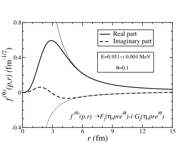
Figure 1: Thick curves: Real and imaginary parts of the complex rotated radial wave function of the $2^{-}$ resonance in ¹⁶F obtained with a box boundary condition. Thin curves: Correct asymptotics of the radial wave function as given by Eq.(2).

In Fig.1 the thick-solid and thick-dashed curves show the real and imaginary parts of the complex rotated radial wave function of the resonance. As mentioned above, in this case the asymptotics is well known, as is given by Eq.(2) with $\xi=\ell$ and $\eta=\frac{\mu c}{p}Z_{1}Z_{2}\alpha$, where $Z_{1}$ and $Z_{2}$ are the charges, $\alpha$ is the fine structure constant, and $p=\sqrt{2\mu E/\hbar}$. This asymptotic behaviour is shown in Fig.1 by the corresponding thin curves. We can see that the numerical radial wave functions, obtained with a simple box boundary condition, reproduce the correct asymptotic behaviour.

4 THREE-BODY CASE

After testing the method for two-body systems, we now use the same procedure for three-body systems, for which the wave functions are computed by using the hyperspheric adiabatic expansion method [3]. In this method the different radial wave functions are obtained by solving the coupled set of differential equations:

$$\left(-\frac{d^{2}}{d\rho^{2}}-\frac{2mE}{\hbar^{2}}+\frac{\lambda_{n}(\rho)+\frac{15}{4}}{\rho^{2}}-Q_{nn}\right)f_{n}(\rho)+\sum_{n^{\prime}\neq n}\left(-2P_{nn^{\prime}}(\rho)\frac{d}{d\rho}-Q_{nn^{\prime}}(\rho)\right)f_{n^{\prime}}(\rho)=0$$ (4)

where $\rho$ is the hyperradius, $m$ is a normalization mass, and $P_{nn^{\prime}}$ and $Q_{nn^{\prime}}$ are the non-adiabatic terms coupling the different radial wave functions [3].

In the previous equations the key quantities are the effective potentials $\lambda_{n}(\rho)$ that are obtained as the eigenvalues of the angular part of the Faddeev equations [3]. Accurate calculation of these eigenvalues is the first and essential requirement needed to obtain reliable radial wave functions.

4.1 2⁺ resonances in ⁶Be and ⁶Li

The main properties of ⁶He are accurately described when treating this nucleus as a three-body system made by an $\alpha$-particle and two neutrons. Since both the alpha-neutron and the neutron-neutron interactions are well known, this nucleus appears as an almost perfect test for all the available numerical three-body methods.

For the same reason, ⁶Be ($\alpha$+$p$+$p$) and ⁶Li ($\alpha$+$n$+$p$) are specially appropriate to investigate three-body systems when more than one particle is charged. In particular, it is well established that ⁶He has a 2⁺ resonance with energy and width ($E_{R}$,$\Gamma_{R}$)=(0.83,0.11) MeV. The same analog $2^{+}$ state has been found in ⁶Li and ⁶Be at (1.67,0.54) MeV and (3.04,1.16) MeV, respectively [4]. Realistic detailed calculations using the (complex scaled) adiabatic expansion method concerning the 2⁺ resonance in ⁶He can be found in [5, 6].

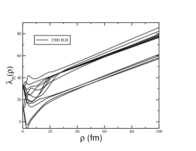
Figure 2: Converged $\lambda$-functions (see Eq.(4)) included in the calculation of the 2⁺ resonance in ⁶Be.

Figure 3: The same as in Fig.3 for the 2⁺ resonance in ⁶Li.

In Figs. 3 and 3 we show the $\lambda$-functions used in the calculation of the 2⁺ resonance in ⁶Be and ⁶Li, respectively. Partial waves with $\ell_{x}$ and $\ell_{y}$ up to 10 have been included. A maximum value of the hypermomentum ($K=2n+\ell_{x}+\ell_{y}$) equal to 20 has been used for all the components, but for the most relevant ones the maximum value of $K$ has been increased up to 200 for $s$-waves, 90 for $p$-waves, and 60 for $d$-waves. In total, slightly more than 2500 hyperspherical harmonics have been included in the calculation. The computed $\lambda$’s have then converged at least up to 100 fm. A reduction by a factor of 2 in the basis size produces $\lambda$-functions indistinguishable from the ones shown in the figures.

It is important to note that ⁶Li, contrary to ⁶Be and ⁶He, is not borromean (the neutron and the proton can bind into deuteron). This is actually revealed by the lowest $\lambda$ in Fig.3, that diverges parabolically to $-\infty$. Therefore, the calculation for ⁶Li requires additional components that are forbidden in ⁶Be and ⁶He. These components correspond to the ones with zero isospin in the neutron-proton channel.

Once the $\lambda$-functions have been computed, the remaining step is to solve the coupled set of differential equations (4). According to the discussion in the previous section, after complex scaling a box boundary condition $f_{n}(\rho_{max})$=0 should be enough to obtain accurate three-body resonance wave functions. However, as shown in Figs.3 and 3 the effective potentials entering in Eq.(4) have been accurately computed only up to $\rho_{max}$=100 fm, that is too little to expect the box boundary condition to work. Furthermore, accurate computation of the $\lambda$’s up to a $\rho_{max}$ value several times larger is too expensive from the computation time point of view.

Figure 4: Real parts of the radial resonance wave functions of the 2⁺ resonance in ⁶Be.

Figure 5: The same as in Fig.5 for the 2⁺ resonance in ⁶Li.

It is not difficult to see [3] that at large distances the $\lambda$-functions go linearly with $\rho$ (this is actually obvious from Figs. 3 and 3). Also the $Q_{nn}$ functions entering in Eq.(4) go like $1/\rho^{2}$, while $P_{nn^{\prime}}$,and $Q_{nn^{\prime}}$ ($n\neq n^{\prime}$) go to zero faster. We have then, for $\rho$ larger than 100 fm, used extrapolations of the $\lambda$’s, $P$’s and $Q$’s in Eq.(4) according to $\lambda_{n}(\rho)=A_{\lambda_{n}}\rho+B_{\lambda_{n}}+C_{\lambda_{n}}/\rho$, $Q_{nn}(\rho)=A_{Q_{nn}}/\rho^{2}+B_{Q_{nn}}/\rho^{3}+C_{Q_{nn}}/\rho^{4}$, and as $A_{P,Q}/\rho^{3}+B_{P,Q}/\rho^{4}+C_{P,Q}/\rho^{5}$ for the non-diagonal $P$’s and $Q$’s. We have then solved the coupled equations (4) using the numerical $\lambda$’s in Figs. 3 and 3 up to 100 fm, and the extrapolations for larger $\rho$’s. In Figs. 5 and 5 we show the real parts of the complex scaled radial wave functions obtained in this way for the $2^{+}$ resonance in ⁶Be and ⁶Li, respectively. For ⁶Be we use a complex scaling angle of 0.15 rads, and $\rho_{max}$=700 fm is enough to obtain a 2⁺ resonance with energy and width ($E_{R}$,$\Gamma_{R}$)=(2.94,1.45) MeV, that agree rather well with the experimental values [4]. For ⁶Li the complex scaling angle is 0.10 rads and $\rho_{max}$=1000 fm. We obtain ($E_{R}$,$\Gamma_{R}$)=(1.67,0.50) MeV, that also agrees well with the experiment [4]. From the figures it is now clear that 100 fm is certainly not large enough to impose a box boundary condition at that distance.

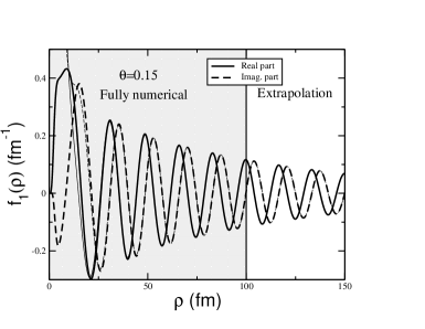
Figure 6: First computed radial wave function (thick curves) for the 2⁺ resonance in ⁶Be and the corresponding asymptotics (thin curves).

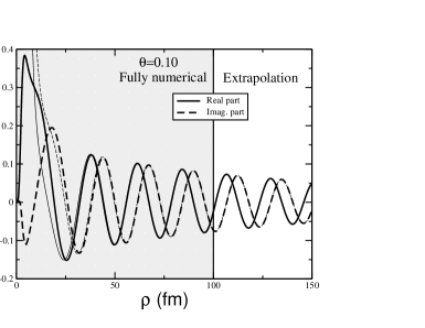
Figure 7: The same as in Fig.7 for the 2⁺ resonance in ⁶Li.

In the extrapolated region ($\rho>100$ fm) the effective potentials entering in Eq.(4) go like $A/\rho+B/\rho^{2}+\cdots$, where the $A$ and $B$ coefficients are computed numerically. For such a kind of potential the solutions are known to go asymptotically as in Eq.(2), where $\xi$ and $\eta$ are easily related to $A$ and $B$. In Figs. 7 and 7 we show the first radial wave function for the $2^{+}$ resonance in ⁶Be and ⁶Li, respectively. The thick curves are the numerical solutions, while the thin curves show the analytic asymptotic behaviour as given by Eq.(2). As seen in both figures the matching with the numerical calculations is very good in the “extrapolated” region, as expected. The remarkable fact is that this agreement is also excellent already around 50 fm, in the region where the purely numerical effective potentials are used.

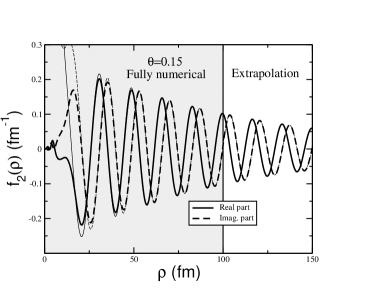
Figure 8: Second computed radial wave function (thick curves) for the 2⁺ resonance in ⁶Be and the corresponding asymptotics (thin curves).

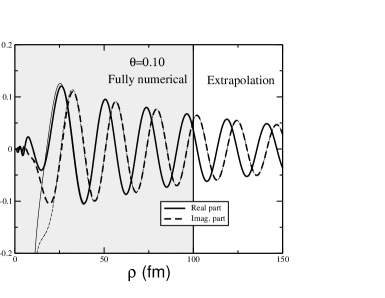
Figure 9: The same as in Fig.9 for the 2⁺ resonance in ⁶Li.

In Figs. 9 and 9 we observe how the same behaviour appears for the second radial wave function. Similar results are also found for the other radial functions. Therefore the numerical resonance radial wave functions obtained with the converged effective potentials shown in Figs. 3 and 3, are consistent with the extrapolations used for the $\lambda$’s, $P$’s and $Q$’s in Eq.(4), and also these solutions have converged to the expected asymptotic behaviour already at $\rho$-values around 50 fm, in the region where full accurate numerical calculations can be performed.

5 SUMMARY AND CONCLUSIONS

After a complex scaling transformation resonance wave functions behave asymptotically as bound states, i.e. falls off exponentially. In this work we exploit this fact to obtain resonances simply by using a box boundary condition at a sufficiently large distance. In this way prior knowledge of the correct asymptotic behaviour of the wave function is not required, permitting then to compute resonances for systems for which this asymptotics is not known, in particular for three-body systems involving more than one charged particle.

After testing the two-body case (for which the correct asymptotics is known), we have investigated the case of the 2⁺ resonance in ⁶Be and ⁶Li. These two nuclei are specially appropriate, since the uncertainties coming from the two-body interactions are small. The (complex scaled) hyperspheric adiabatic expansion method is used. Accurate and converged effective potentials are obtained up to $\rho_{max}$=100 fm, and beyond this distance extrapolations are used. These extrapolations permit to know the correct asymptotic behaviour, that should be the right one at least for distances much larger than $\rho_{max}$.

When solving the radial equations with a box boundary condition at a large value of $\rho$ (700 fm for ⁶Be and 1000 fm for ⁶Li) we have found that at rather modest distances ($\rho\approx$50 fm) the radial wave functions already match with the asymptotic behaviour obtained from the extrapolated effective potentials. This means that the numerical effective potentials obtained for $\rho<\rho_{max}$ are consistent with the extrapolations used to solve the radial equations. Furthermore, use of these numerical potentials is enough to obtain radial resonance wave functions that have already reached the asymptotic behaviour. This implies that observables related to the asymptotics of the wave functions can be safely computed using the resonance wave functions obtained by this procedure. An example is the energy distributions of the fragments after decay of the resonance. The experimental energy distributions are related to the energy distributions of the fragments at distances where the correct asymptotics has been reached [7].

References

- [1] E. Garrido, D.V. Fedorov, A.S. Jensen, Nucl. Phys. A 733 (2004) 85.
- [2] F. Ajzenberg-Selove, Nucl. Phys. A 460 (1986) 1.
- [3] E. Nielsen, D.V. Fedorov, A.S. Jensen, E. Garrido, Phys. Rep. 347 (2001) 373.
- [4] F. Ajzenberg-Selove, Nucl. Phys. A 490 (1988) 1.
- [5] D.V. Fedorov, E. Garrido, A.S. Jensen, Few-Body Syst. 33 (2003) 153.
- [6] E. Garrido, D.V. Fedorov, A.S. Jensen, H.O.U. Fynbo, Nucl. Phys. A 766 (2006) 74.
- [7] D.V. Fedorov, H.O.U. Fynbo, E. Garrido, A.S. Jensen, Few-Body Syst. 34 (2004) 33.