Static properties of nuclear matter within the Boson Loop Expansion

Abstract

The use of the Boson Loop Expansion is proposed for investigating the static properties of nuclear matter. We explicitly consider a schematic dynamical model in which nucleons interact with the scalar–isoscalar $\sigma$ meson. The suggested approximation scheme is examined in detail at the mean field level and at the one– and two–loop orders. The relevant formulas are provided to derive the binding energy per nucleon, the pressure and the compressibility of nuclear matter. Numerical results of the binding energy at the one–loop order are presented for Walecka’s $\sigma$-$\omega$ model in order to discuss the degree of convergence of the Boson Loop Expansion.

1 Introduction

Functional integral methods have been extensively used over the years to provide useful approximation schemes in many different areas of physics, in both the perturbative and the non–perturbative regimes [1, 2, 3, 4, 5, 6]. The nuclear many–body problem has been widely investigated starting from renormalizable, relativistic Lagrangians based on the so–called quantum hadrodynamics (QHD) [7]: calculation schemes have been explored, which go beyond the tree–level approximation and thus involve the dynamics of the quantum vacuum. Being a strong–coupling model, no obvious asymptotic expansion exists for QHD. Hence it is not guaranteed that a reliable, convergent expansion, allowing for systematic refinements of the theoretical predictions, exists for this model.

Some approaches are based on the so–called Loop Expansion, which can be derived from the exact path integral formulation of QHD [4]: it is obtained by expanding the QHD effective action around its classical value and by considering terms with increasing number of quantum loops [1, 2]. Formally, the resulting Loop Expansion is thus a power series in $\hbar$, though Planck’s constant is merely a bookkeeping parameter [2]. One can also consider it as a perturbative expansion in powers of the coupling constants $g_{\sigma}$, $g_{\omega}$, etc, but keeping in mind that it is non–perturbative in the mean fields, since it involves Hartree–dressed nucleon propagators. The one–loop approximation of the Loop Expansion corresponds to the Relativistic Hartree Approximation [8]. In Refs. [9] full two–loop corrections were evaluated for QHD-I (i.e., Walecka’s $\sigma$-$\omega$ model) and criteria for “strong” and “weak” convergence were discussed. Two–loop terms involving the vector meson $\omega$ were found to be too attractive for standard values of the coupling constant $g_{\omega}$, thus making two–loop corrections to the nuclear matter binding energy too large with respect to the well known mean field results. This result precluded strong convergence. After tuning the QHD-I parameters, the correct saturation point of nuclear matter at the two–loop order was obtained at the price of drastically reducing $g_{\omega}$. At the same time $g_{\sigma}$ was significantly increased, the dynamics of the system being led almost entirely by the scalar $\sigma$ meson. It was thus concluded that, at two–loop order, the Loop Expansion is not even weakly convergent.

To suppress the unwanted high–momentum structure of the hadronic vacuum loops, short–range correlations and vertex corrections have also been considered in calculations at the two–loop order [10, 11, 12]. These investigations showed a clear improvement over the results of Ref. [9], which were carried out with structureless nucleons. Although obtained with a “reasonable” fit of the coupling constants, the results turned out to have a strong dependence on the model, not phenomenologically constrained, adopted for the short–range correlations or the vertex corrections. Moreover, the renormalizability of the theory was lost.

The above failure of the Loop Expansion could be due to its inability in describing the quantum vacuum dynamics. Indeed it is derived as a perturbative expansion in the “large” QHD-I couplings, while “small” couplings are required to assure some convergence of the Loop Expansion predictions [13]. One could also claim that the QHD model itself, based on point–like hadrons, is not appropriate to include quantum vacuum effects.

In order to test the validity of these hypotheses, alternative loop expansions based on QHD, non–perturbative in both the couplings and the mean fields, should be studied. In this context we mention here the so–called Modified Loop Expansion or Boson Loop Expansion, which is an example of a non–perturbative approach and in addition preserves renormalizability.

The Modified Loop Expansion, first introduced by Weiss [15], has been later employed in Ref. [16] together with a chirally symmetric linear $\sigma$ model for nuclear matter calculations. In this approach, fermionic degrees of freedom are integrated out in the generating functional. This leads to an effective action in which meson loops are included order by order in $\hbar$ and, at each order $\hbar^{n}$ in the meson loops, baryon loops are summed to all orders in $\hbar$. The zeroth–order of this expansion corresponds to the Relativistic Hartree Approximation, the modified one–loop level to the Relativistic Random Phase Approximation. Hence the first–order Modified Loop Expansion corresponds to the two–loop level of the Loop Expansion, but with meson propagators dressed in Random Phase Approximation. We are not aware of detailed calculations applying this scheme to QHD-I.

The so–called Boson Loop Expansion (BLE), which we shall consider in the present paper, has been proposed as a suitable tool to formulate consistent approximation schemes for non–perturbative calculations in different issues of nuclear physics [17, 18, 19, 20, 21, 22, 23]. The underlying idea, as in MLE, amounts to integrate out the nucleonic degrees of freedom within a path–integral formulation for the dynamics of interacting nucleons and mesons. The loop expansion is then carried out on the resulting bosonic effective action. This approach has been applied to the calculation of the electromagnetic nuclear response functions and provided a suitable framework to understand the reaction mechanisms [21]. It has also been successfully used for the evaluation of the hypernuclear weak decay rates [23].

Actually, while the BLE has the merit of rigorously preserving sum rules and general field theory theorems, the underlying dynamics still needs to be more firmly settled. We intend to apply this method to the investigation of other observables, such as the static properties of nuclear matter and neutron stars, topics of considerable interest and yet under debate after decades of valuable works. It is worth noticing that this approach is particularly suited to deal with a relativistic description and, in addition, it is stable against sizable increases of the nuclear density.

Particular attention has to be payed to the adopted dynamical model. In a relativistic frame, QHD models are often employed at face to calculations based on realistic nucleon–nucleon potentials like the Bonn meson exchange model [24]. These two schemes started from quite different points of view and originally provided sizably different results: however in recent times the evolution of calculations in both approaches has significantly reduced the gap. QHD is mainly based on the $\sigma$-$\omega$ interference, while the Bonn potential, in addition to the exchange of several physical mesons, replaces the $\sigma$ meson exchange with a two–pion exchange together with the simultaneous excitation of one or two intermediate nucleons to $\Delta$ resonances (box diagrams). From a phenomenological point of view, this seems to favor the Bonn approach for the calculation of the equation of state of nuclear matter. However, a $G$–matrix calculation based on the Bonn potential is quite cumbersome and some self–consistency effect of relativistic origin is generally neglected. In this context, calculations are usually limited to the Lowest Order Brückner Theory, which implies lowest order in the nuclear density; this limitation is acceptable in ordinary nuclear matter calculations, but less so in addressing dense baryonic matter such as in neutron stars.

In order to clarify the fundamental problems underlying the BLE (namely the issue concerning the renormalization procedure), in this paper we develop the formalism within a simple dynamical model containing nucleons and $\sigma$ mesons only. We shall provide the relevant formulas which are needed to derive the static properties of nuclear matter up to the two–boson–loop level. In view of a future, comprehensive application to QHD, as well as to give a first insight on the convergence properties of the proposed expansion, here we present numerical results for the nuclear matter binding energy at the one–loop order when adopting a $\sigma$-$\omega$ model. The complete BLE formalism for QHD-I, together with systematic numerical calculations up to the two–loop order, will be presented in a forthcoming paper, also devoted to discuss the phenomenological aspects of the present approach.

The paper is organized as follows. Section 2 contains a brief introduction to the general formalism employed in the functional approach for the evaluation of the static properties of nuclear matter. In Section 3 a bosonic effective action is derived for a system of interacting nucleons and $\sigma$ mesons. The “elementary” vertices entering into this effective action are analyzed in some detail in Section 4. In Section 5 the renormalization procedure for the bosonic action is carried out. In Section 6 we deduce the BLE as a Semiclassical expansion around the (mean field) solution given by the stationary phase approximation. Some numerical results for the $\sigma$-$\omega$ model are presented in Section 7. Finally, in Section 8 we comment on the future perspectives opened by the present work.

2 The functional method – General formalism

To construct the formalism we consider a simplified situation where a scalar–isoscalar meson (the $\sigma$) interacts with a massive fermion field (the nucleon). The introduction of the $\omega$ meson, to complete the standard scheme of QHD induces a mixing with the $\sigma$ meson and a problem of renormalizability, which can be solved by means of the so–called Stueckelberg gauge [25] and not simply invoking the current conservation, as usually stated [7]; this will be discussed in a forthcoming paper. We shall see in the following that already the “simple” scalar field needs a careful renormalization procedure.

The most general Lagrangian density reads

$$\begin{split}{\mathcal{L}}&=\overline{\psi}(i\hbox to0.0pt{/\hss}\partial-m)\psi+\frac{1}{2}\partial_{\mu}\sigma\,\partial^{\mu}\sigma-\frac{1}{2}m_{\sigma}^{2}\sigma^{2}+g\overline{\psi}\sigma\psi-U(\sigma)\\ &=\int d^{4}y\,\overline{\psi}(x)S^{-1}_{0}(x-y)\,\psi(y)+\frac{1}{2}\int d^{4}y\,\sigma(x)D^{-1}_{0}(x-y)\,\sigma(y)\\ &+g\,\overline{\psi}(x)\sigma(x)\psi(x)-U[\sigma(x)]\,,\end{split}$$ (1)

the two expressions differing by an irrelevant four–divergence. In the above

$$S^{-1}_{0}(x-y) = (i\hbox to0.0pt{/\hss}\partial_{x}-m)\,\delta^{4}(x-y)~{},$$ (2)

$$D^{-1}_{0}(x-y) = -(\Box_{x}+m^{2}_{\sigma})\,\delta^{4}(x-y)~{},$$ (3)

formally define the free nucleon and $\sigma$ propagators, $S_{0}$ and $D_{0}$ respectively, in coordinate space, and

$$U(\sigma)=\frac{\lambda_{3}}{3!}\sigma^{3}+\frac{\lambda_{4}}{4!}\sigma^{4}=\frac{b\,m\,g^{3}}{3}\sigma^{3}+\frac{c\,g^{4}}{4}\sigma^{4}\,.$$ (4)

In momentum space the nucleon propagator in nuclear matter with Fermi momentum $k_{F}$ and the free $\sigma$ propagator read, respectively:

$$S_{0}(k)=\frac{\hbox to0.0pt{/\hss}k+m}{2E_{k}}\left\{\frac{\theta(|{\bf k}|-k_{F})}{k_{0}-E_{k}+i\eta}+\frac{\theta(k_{F}-|{\bf k}|)}{k_{0}-E_{k}-i\eta}-\frac{1}{k_{0}+E_{k}-i\eta}\right\}~{},$$ (5)

$$D_{0}(q)=\frac{1}{q^{2}-m_{\sigma}^{2}+i\epsilon}~{},$$ (6)

where $E_{k}=\sqrt{{\bf k}^{2}+m^{2}}$. It is also useful to introduce a symbol for the free fermion propagator in the vacuum, $S_{0v}\equiv\left.S_{0}\right|_{k_{F}=0}$, thus splitting Eq. (5) as follows

$$S_{0}(k) = S_{0v}(k)+S_{0M}(k)~{},$$ (7)

$$S_{0v}(k) = \frac{1}{\hbox to0.0pt{/\hss}k-m+i\eta}~{},$$ (8)

$$S_{0M}(k) = (\hbox to0.0pt{/\hss}k+m)\frac{i\pi}{E_{k}}\theta(k_{F}-|{\bf k}|)\delta(k_{0}-E_{k})~{},$$ (9)

the latter being the density–dependent part.

The classical action corresponding to the Lagrangian (1) is given by:

$${\mathcal{A}}[\bar{\psi},\psi,\sigma]=\int d^{4}x\,{\mathcal{L}}(\bar{\psi}(x),\psi(x),\sigma(x))~{},$$ (10)

where the $\sigma$ and nucleon fields have to be interpreted as scalar and Grassmann variables respectively. In a path integral approach the whole dynamics is deduced from the generating functional

$$Z[\bar{\eta},\eta,J]=\frac{1}{{\mathcal{N}}}\int D[\bar{\psi},\psi,\sigma]\,e^{\,i\left\{{\mathcal{A}}[\bar{\psi},\psi,\sigma]+\int d^{4}x\left[\bar{\psi}(x)\eta(x)+\bar{\eta}(x)\psi(x)+\sigma(x)J(x)\right]\right\}}~{},$$ (11)

where $\mathcal{N}$ is a normalization constant while $\eta$, $\bar{\eta}$ and $J$ denote the external (classical) sources of the nucleon and $\sigma$ meson fields. From $Z$ one derives the nucleon Green’s functions by functional differentiations with respect to $\eta$ and $\bar{\eta}$. The $\sigma$ Green’s function is obtained by derivatives with respect to $J$. Other external sources coupled to composite fields could also be added: for instance, couplings of the kind $\bar{\psi}(x)\psi(x)\rho(x)$ permit the evaluation of the response function through a double derivative of $Z$ with respect to $\rho$.

The static properties of the system follow from the partition function $Z(\beta)$ which can be obtained from the generating functional of Eq. (11) by:

1. setting the external sources to 0;

2. performing a Wick rotation, namely replacing, in the exponent, the time integration (extended from $-\infty$ to $\infty$) with an integration over the imaginary time $\tau=it$ in the interval $[0,\beta]$ with $\beta\equiv\hbar/(k_{B}T)=1/T$;

3. replacing the Hamiltonian $\hat{H}=\int d^{3}x\,{\mathcal{H}}(x)$ with $\hat{H}-\mu\hat{N}$, $\mu$ being the nucleon chemical potential and $\hat{N}=\int d^{3}x\,\bar{\psi}(x)\gamma^{0}\psi(x)$ the nucleon number operator;

4. setting ${\mathcal{N}}=1$.

By applying these rules, one gets

$$Z(\beta)={\rm Tr}\,e^{-\beta(\hat{H}-\mu\hat{N})}=\int D[\bar{\psi},\psi,\sigma]e^{\,\,\int\limits_{0}^{\beta}d\tau\int d^{3}x\,{\mathcal{L}}_{E}(\tau,{\bf x})}~{}.$$ (12)

The Euclidean Lagrangian ${\mathcal{L}}_{E}$ is obtained by replacing $t$ with $-i\tau$ in the Minkowskian Lagrangian (1) and reads

$$\begin{split}{\mathcal{L}}_{E}(\tau,\mathbf{x})\equiv{\mathcal{L}}_{E}(\bar{x})&=\int d^{4}\bar{y}\,\overline{\psi}(\bar{x})S^{-1}_{0E}(\bar{x}-\bar{y})\psi(\bar{y})\\ &+\frac{1}{2}\int d^{4}\bar{y}\,\sigma(\bar{x})D^{-1}_{0E}(\bar{x}-\bar{y})\sigma(\bar{y})+g\,\overline{\psi}(\bar{x})\sigma(\bar{x})\psi(\bar{x})-U[\sigma(\bar{x})]\\ &\equiv-\left[{\mathcal{H}}(\bar{x})-\mu\,\overline{\psi}(\bar{x})\gamma^{0}\psi(\bar{x})\right]~{},\end{split}$$ (13)

where we have denoted the Euclidean space–time coordinates with an upper bar [$\bar{x}=(\tau,\mathbf{x})$, $\bar{y}=(\tau_{y},\mathbf{y})$] and ${\mathcal{H}}$ is the (Euclidean) Hamiltonian density. In the zero temperature limit $S^{-1}_{0E}$ and $D^{-1}_{0E}$ are given by

$$S^{-1}_{0E}(\bar{x}-\bar{y}) = -(\gamma^{0}\partial_{\tau_{x}}+i\,{\boldsymbol{\gamma}}\cdot{\mathbf{\nabla}}_{x}+m)\,\delta^{4}(\bar{x}-\bar{y})~{},$$ (14)

$$D^{-1}_{0E}(\bar{x}-\bar{y}) = -(-\partial^{2}_{\tau_{x}}-{\mathbf{\nabla}}_{x}^{2}+m^{2}_{\sigma})\,\delta^{4}(\bar{x}-\bar{y})~{}.$$ (15)

The Euclidean propagators in momentum space follow from Eqs. (5),(6) with the replacements $k_{0}\to ik_{0}+\mu$ and $q_{0}\to iq_{0}$ and take the form

$$S_{0E}(k) = \frac{1}{\gamma_{0}(ik_{0}+\mu)-{\boldsymbol{\gamma}}\cdot{\bf k}-m}~{},$$ (16)

$$D_{0E}(q) = -\frac{1}{q_{0}^{2}+{\bf q}^{2}+m_{\sigma}^{2}}~{}.$$ (17)

Once the partition function $Z(\beta)$ is known, the ground state ($T=0$) energy of nuclear matter follows from the relation

$$E\equiv\langle\hat{H}\rangle=\lim_{\beta\to\infty}\left(-\frac{\partial}{\partial\beta}\log Z(\beta)+\mu A\right)=\lim_{\beta\to\infty}\left(-\frac{\log Z(\beta)}{\beta}+\mu A\right)~{},$$ (18)

$A\equiv\langle\hat{N}\rangle$ being the total number of nucleons. Note that the nucleon chemical potential is related to the Fermi momentum by

$$\lim_{\beta\to\infty}\mu=E_{F}^{*}\equiv\sqrt{k_{F}^{2}+(m^{*})^{2}}~{},$$ (19)

where $m^{*}$ is the nucleon effective mass at the mean field level [see Eq. (38)] and follows from the dynamics underlying the Lagrangian (1). In the next Section we shall introduce an approximate scheme to evaluate the ground state energy and therefore the binding energy per nucleon:

$$\frac{B.E.}{A}\equiv\frac{E}{A}-m\equiv\frac{\epsilon}{\rho}-m~{},$$ (20)

where $\epsilon\equiv E/\Omega$ and $\rho\equiv A/\Omega=2k_{F}^{3}/(3\pi^{2})$ are the energy density and the number density of nuclear matter, respectively. Note that we are implicitly considering symmetric nuclear matter ($k_{F_{n}}=k_{F_{p}}=k_{F}$) but all our results can be easily adapted to the asymmetric case.

Once $\epsilon$ is known, other observables are accessible. Pressure (and hence the equation of state) and compressibility are indeed given by the thermodynamical relations:

$$P=\rho^{2}\frac{\partial}{\partial\rho}\left(\frac{\epsilon}{\rho}\right)=-\epsilon+\rho\frac{\partial\epsilon}{\partial\rho}~{},$$ (21)

and

$${\mathcal{K}}=9\frac{\partial P}{\partial\rho}=9\rho\frac{\partial^{2}\epsilon}{\partial\rho^{2}}~{}.$$ (22)

Other quantities, such as for instance the symmetry energy, could also be addressed, but they involve the dynamics of isovector mesons, which has been recently studied in Refs. [26, 27], and will be considered by us in future investigations.

Within the present path integral method, the problem of evaluating the static properties of nuclear matter requires the elaboration of approximation techniques in order to compute the functional integral which defines the partition function (12).

3 The Bosonic Effective Action

As stated in the Introduction, we shall concentrate here on the approximation scheme given by the Boson Loop Expansion [17, 21]. As a first step to derive it, one has to introduce a bosonic effective action corresponding to the Lagrangian density (1) but no longer displaying fermionic degrees of freedom. This is the specific purpose of the present Section.

At variance with Ref. [8], we present the theory in a heuristic way, disregarding in the present Section the renormalization problem and the $\sigma$ self–interaction terms —which in turn add non-trivial complications to the renormalization problem— and leaving for a second step (Sec. 6) the details of the renormalization procedure; the latter, indeed, affects the binding energy in the medium already at the mean field level [8]. We also notice that the classification of the counterterms in the usual Loop Expansion and in the BLE is different.

Since we shall focus our attention only on the boson–like observables of Eqs. (18)–(22), we can safely put $\bar{\eta}=\eta=0$ in the generating functional of Eq. (11). The functional integral is then converted into an integral over bosonic variables only, by explicitly integrating out the fermionic field; one obtains

$$Z[J]=\frac{1}{{\mathcal{N}}}\int D[\sigma]\,e^{\,iA^{B}_{\rm eff}[\sigma]+i\int d^{4}x\,\sigma(x)J(x)}~{}.$$ (23)

By using well known properties of the following Gaussian integral over Grassmann variables:

$$\int D[\bar{x},x]\;e^{-\bar{x}Ax}=\det A=e^{{\rm Tr}\log A}~{},$$

the bosonic effective action $A^{B}_{\rm eff}$ entering into Eq. (23) turns out to be

$$A^{B}_{\rm eff}[\sigma] = \frac{1}{2}\int d^{4}x\,d^{4}y\,\sigma(x)D_{0}^{-1}(x-y)\sigma(y)-i{\rm Tr}\log[-i(S_{0}^{-1}+g\sigma)]$$

$$= \frac{1}{2}\int d^{4}x\,d^{4}y\,\sigma(x)D_{0}^{-1}(x-y)\sigma(y)+A^{B}_{0}+i{\rm Tr}\sum_{n=1}^{\infty}\frac{(-1)^{n}}{n}\left[S_{0}g\sigma\right]^{n}$$

$$= \frac{1}{2}\int d^{4}x\,d^{4}y\,\sigma(x)D_{0}^{-1}(x-y)\sigma(y)+A^{B}_{0}-i{\rm Tr}\int\limits_{0}^{g}\frac{d\lambda}{\lambda}\frac{\lambda\sigma}{S_{0}^{-1}+\lambda\sigma}~{}.$$

The term

$$A^{B}_{0}=-i{\rm Tr}\log[-iS_{0}^{-1}]$$ (25)

is related to the functional generator of non–interacting fermions by

$$e^{iA^{B}_{0}}=\int D[\bar{\psi},\psi]e^{i\int d^{4}x\,d^{4}y\,\bar{\psi}(x)S_{0}^{-1}(x-y)\psi(y)}~{}.$$ (26)

Let us stress that, although the fermionic degrees of freedom have been integrated out, their influence on the generating functional (23) remains unaltered.

Note that in (3) space–time integrals are also contained in the traces, in addition to a sum over spin and isospin. The trace of the logarithm acquires a meaning only through its series expansion (second line of Eq. (3)). Moreover ${\rm Tr}[S_{0}g\sigma]^{n}$ is a short notation for

$${\rm Tr}[S_{0}g\sigma]^{n}=4g^{n}\int d^{4}x_{1}\dots d^{4}x_{n}\,{\mathfrak{P}}^{(n)}_{0}(x_{1},\dots,x_{n})\sigma(x_{1})\sigma(x_{2})\dots\sigma(x_{n})~{},$$ (27)

where we have defined

$${\mathfrak{P}}^{(n)}_{0}(x_{1},\dots,x_{n})=S_{0}(x_{1}-x_{2})S_{0}(x_{2}-x_{3})\dots S_{0}(x_{n}-x_{1})\,,$$ (28)

and the factor 4 originates from the spin–isospin trace.

It will be also useful to introduce the vertices ${\mathfrak{P}}^{(n)}_{0}$ evaluated in the vacuum, denoted by ${\mathfrak{P}}^{(n)}_{0v}$: they are obtained from Eq. (28) with the replacement $S_{0}\to S_{0v}$, while the corresponding density–dependent contributions are ${\mathfrak{P}}^{(n)}_{0M}={\mathfrak{P}}^{(n)}_{0}-{\mathfrak{P}}^{(n)}_{0v}$.

Their Fourier transforms are also needed. Here the independent variables are $n-1$ and we get

$$\widetilde{\mathfrak{P}}^{(n)}_{0}(p_{1},p_{2},\dots p_{n-1})=$$ (29)

$$\quad-i\int\frac{d^{4}p}{(2\pi)^{4}}S_{0}(p)S_{0}(p+p_{1})S_{0}(p+p_{1}+p_{2})\dots S_{0}(p+p_{1}+\dots+p_{n-1})\,.$$

The Euclidean version of the bosonic effective action is

$$A^{B}_{E\,\rm eff}(\beta) ={\rm Tr}\log[-S^{-1}_{0E}]+\tilde{A}^{B}_{E\,\rm eff}(\beta)~{},$$ (30)

$$\tilde{A}^{B}_{E\,\rm eff}(\beta) =\frac{1}{2}\int d^{4}\bar{x}\,d^{4}\bar{y}\,\sigma(\bar{x})D^{-1}_{0E}(\bar{x}-\bar{y})\sigma(\bar{y})-{\rm Tr}\sum_{n=1}^{\infty}\frac{(-1)^{n}}{n}\left[S_{0E}g\sigma\right]^{n}$$

$$=\frac{1}{2}\int d^{4}\bar{x}\,d^{4}\bar{y}\,\sigma(\bar{x})D^{-1}_{0E}(\bar{x}-\bar{y})\sigma(\bar{y})+{\rm Tr}\int\limits_{0}^{g}\frac{d\lambda}{\lambda}\frac{\lambda\sigma}{S_{0E}^{-1}+\lambda\sigma}~{},$$

and the partition function takes the form

$$Z(\beta)=Z_{0}(\beta)\int D[\sigma]\,e^{\tilde{A}^{B}_{E\,\rm eff}(\beta)}~{}.$$ (31)

Here,

$$Z_{0}(\beta)=\det[-S^{-1}_{0E}]=\int D[\bar{\psi},\psi]\,e^{\,\,\int d^{4}\bar{x}\,d^{4}\bar{y}\,\bar{\psi}(\bar{x})S_{0E}^{-1}(\bar{x}-\bar{y})\psi(\bar{y})}$$ (32)

is the partition function for an assembly of non–interacting nucleons and the remaining functional integral in Eq. (31) represents a system of self–interacting bosons.

The interaction terms of Eq. (27) are built up with closed fermionic loops, either in the Minkowskian or Euclidean space, and play a central role in the present treatment. It has been shown in Refs. [18, 28] that, within a non–relativistic kinematics, they can be either evaluated explicitly or at least reduced to the evaluation of a one–dimensional integral. Note however that the difficulties met in Refs. [18, 28] mainly derived from the kinematical singularities in Eq. (27). The use of the Euclidean metric shifts all of them in the complex plane, considerably simplifying the numerical integrations. Since these interaction terms represent the building blocks of the BLE, they require a careful treatment. Relativistic calculations are much more sensitive to the dynamics of the mesons with respect to non–relativistic case. In the latter, indeed, at least in most practical cases, the mesonic dynamics is frozen (the meson exchange is reduced to a static potential) and it is reflected in some spin operators which are easily traced out. On the contrary, in a relativistic approach convective currents cannot be neglected without violating Lorentz covariance. We shall discuss in the next Section how some archetypal cases may be constructed and how one can handle more complicated dynamics.

To evaluate the generating functional (23) or the partition function (31), we adopt the semiclassical expansion. Its lowest order, i.e., the mean field level, corresponds to the stationary phase approximation (saddle point approximation in the Euclidean space). At this stage, one requires the bosonic action to be stationary with respect to small variations of the field $\sigma$:

$$\frac{\delta A^{B}_{\rm eff}[\sigma]}{\delta\sigma}=0~{}.$$ (33)

The following equation of motion is thus obtained:

$$\int d^{4}y\,D_{0}^{-1}(x-y)\sigma(y)=-i{\rm Tr}\sum_{n=1}^{\infty}(-1)^{n}[S_{0}g\sigma]^{n-1}S_{0}g=ig\,{\rm Tr}\,\frac{S_{0}}{1+S_{0}g\sigma}~{}.$$ (34)

One recognizes that $\sigma$ cannot be vanishing at the mean field level, since the first term of the sum in Eq. (34) is just a fermionic line closed onto itself, namely the tadpole

$$ig{\rm Tr}\,S_{0}=4ig\int d^{4}y\,S_{0}(y-y)~{}.$$

The above quantity is obviously divergent but the usual renormalization techniques, described in Sec. 5, make it finite and non–trivial [8, 29]. This occurrence emphasizes the peculiar role played by the scalar–isoscalar field, which is indeed the only one generating a tadpole, even in the vacuum, where any other meson field has vanishing expectation value.

For static, infinite nuclear matter, the mean field solution is uniform in space and time, thus the lhs of the field equation (34) reduces to

$$\int d^{4}y\,D^{-1}_{0}(x-y)\sigma(y)=-\left(\Box_{x}+m^{2}_{\sigma}\right)\sigma(x)=-m^{2}_{\sigma}\bar{\sigma}~{}.$$ (35)

In the “no–sea” approximation, the mean field $\bar{\sigma}$ is then obtained by solving the following self–consistency equation (we introduce the scalar density $\rho_{s}=\langle\bar{\psi}\psi\rangle$ and its density–dependent part $\rho_{sM}=\langle\bar{\psi}\psi\rangle_{M}$):

$$\begin{split}\bar{\sigma}&=\frac{g}{m^{2}_{\sigma}}\rho_{sM}=-i\frac{g}{m_{\sigma}^{2}}{\rm Tr}\,S_{HM}=-4i\frac{g}{m_{\sigma}^{2}}\int\frac{d^{4}k}{(2\pi)^{4}}S_{HM}(k)\\ &=\frac{g}{m_{\sigma}^{2}}\frac{m^{*}}{\pi^{2}}\left(k_{F}E_{F}^{*}-(m^{*})^{2}\log\frac{k_{F}+E_{F}^{*}}{m^{*}}\right)~{},\end{split}$$ (36)

where $S_{HM}$ is the density–dependent part of the Hartree–dressed nucleon propagator

$$S_{H}=\frac{1}{S_{0}^{-1}+g\bar{\sigma}}~{},$$ (37)

that is obtained from the definition of $S_{0}$ in Eq. (5) after replacing $m$ with the nucleon effective mass:

$$m^{*}=m-g\bar{\sigma}\,.$$ (38)

From a diagrammatic point of view, self–consistency amounts to account for diagrams like those of Figure 1, in which each nucleon propagator is dressed by the Hartree self–energy.

Figure 1: Mean field level nucleon self–energy diagrams for $\sigma$ exchange.

In view of an application of the present scheme to QHD, one has to consider the contribution of the vector–isoscalar meson $\omega$ as well. The $\omega$ mean field is obtained as $\bar{\omega}_{\mu}=({g_{\omega}}/{m_{\omega}^{2}})\rho\,\delta_{\mu 0}~{},$ without any self–consistency condition because the nuclear density

$$\rho\equiv\langle\bar{\psi}\gamma_{0}\psi\rangle=2\frac{k^{3}_{F}}{3\pi^{2}}$$

is now implied instead of the scalar density $\rho_{s}$. The relativistic (Lorentz contraction) effect stemming from the difference between the two mean values was already noted long time ago by Lee and Wick [13] and ultimately entails a restoration of the chiral symmetry at sufficiently high density in the Wigner mode.

Since Eq. (36) provides a non–vanishing solution for the mean field $\bar{\sigma}$, in order to apply the standard technique of the Semiclassical approximation one needs to define a new scalar–isoscalar field $\sigma^{\prime}(x)=\sigma(x)-\bar{\sigma}$ with vanishing expectation value at the mean field level, $\bar{\sigma^{\prime}}=0$. By rewriting the generating functional (23) with the above change of variable and then renaming $\sigma^{\prime}$ as $\sigma$, the bosonic effective action (3) becomes

$$A^{B}_{\rm eff}[\sigma]=\frac{1}{2}\sigma D_{0}^{-1}\sigma-\frac{m_{\sigma}^{2}}{2}(2\sigma\bar{\sigma}+{\bar{\sigma}}^{2})+A^{B}_{0}+i{\rm Tr}\sum_{n=1}^{\infty}\frac{(-1)^{n}}{n}[S_{0}g(\sigma+\bar{\sigma})]^{n}$$ (39)

and the coupling to the external field changes to $(\sigma+\bar{\sigma})J$.

Next, one can write

$$i{\rm Tr}\sum_{n=1}^{\infty}\frac{(-1)^{n}}{n}[S_{0}g(\sigma+\bar{\sigma})]^{n}\\ =i{\rm Tr}\sum_{n=1}^{\infty}\frac{(-1)^{n}}{n}[S_{H}g\sigma]^{n}+i{\rm Tr}\sum_{n=1}^{\infty}\frac{(-1)^{n}}{n}[S_{0}g\bar{\sigma}]^{n}~{},$$ (40)

as it can be easily verified keeping in mind Eq. (37) and by rewriting the series in terms of the corresponding $\log$’s. By using Eq. (36), the $n=1$ term in the first sum of the rhs of Eq. (40) reads $-ig{\rm Tr}S_{H}\sigma=m_{\sigma}^{2}\sigma\bar{\sigma}~{},$ so that no linear term in $\sigma$ enters the effective action:

$$A^{B}_{\rm eff}[\sigma]=\frac{1}{2}\sigma D_{0}^{-1}\sigma-\frac{m_{\sigma}^{2}}{2}\bar{\sigma}^{2}\\ +A^{B}_{0}+i{\rm Tr}\sum_{n=2}^{\infty}\frac{(-1)^{n}}{n}[S_{H}g\sigma]^{n}-i{\rm Tr}\log[1+S_{0}g\bar{\sigma}]~{}.$$ (41)

Let us remark that the constant terms in $A^{B}_{\rm eff}$ are irrelevant in evaluating the generating functional, but they are significant in the partition function. By using the definition (25), one can recognize the following reordering

$$A^{B}_{0}-i{\rm Tr}\log[1+S_{0}g\bar{\sigma}]=-i{\rm Tr}\log[-iS_{H}^{-1}]~{}.$$ (42)

We then consider the partition function. The part of the Euclidean action originating from the constant term (42) now replaces the factor $Z_{0}(\beta)$ of Eq. (32). The difference between Eq. (42) and Eq. (25) lies in the replacement $m\to m^{*}$, namely $S_{0E}\to S_{HE}=(S^{-1}_{0E}+g\bar{\sigma})^{-1}$, $S_{HE}$ being the Euclidean version of $S_{H}$. Therefore we can write

$$Z(\beta)=Z_{0}^{*}(\beta)\int D[\sigma]\,e^{\,\widehat{A}^{B}_{E\,\rm eff}(\beta)}~{},$$ (43)

with

$$Z^{*}_{0}(\beta)=\det[-S^{-1}_{HE}]=\int D[\bar{\psi},\psi]\,e^{\int d^{4}\bar{x}\,d^{4}\bar{y}\,\bar{\psi}(\bar{x})S_{HE}^{-1}(\bar{x}-\bar{y})\psi(\bar{y})}~{},$$ (44)

and

$$\widehat{A}^{B}_{E\,\rm eff}(\beta)=\frac{1}{2}\sigma D^{-1}_{0E}\sigma-\Omega\beta\frac{m_{\sigma}^{2}}{2}\bar{\sigma}^{2}-{\rm Tr}\sum_{n=2}^{\infty}\frac{(-1)^{n}}{n}\left[S_{HE}\,g\sigma\right]^{n}~{}.$$ (45)

In this expression, space–time integrations are understood for the free $\sigma$ contribution, but in the second, constant term in the rhs, the time ($\beta$) and volume ($\Omega$) integrations have been made explicit.

4 The elementary vertices of the bosonic action

We analyze now the elementary vertices corresponding to ${\rm Tr}[S_{H}g\sigma]^{n}$ and entering the bosonic effective action (41). When embedded in a Feynman diagram, a term ${\rm Tr}[S_{H}g\sigma]^{n}$ is represented by a fermionic loop with $n$ external points; a boson propagator can be attached to each one of these points, including the spin and isospin matrices which pertain to the specific boson. Isospin traces only factorize out a real number, but the possible presence of $\gamma$ matrices, as it is the case for the $\omega$ exchange, entails a non–trivial dependence upon the momenta, which is usually neglected in non–relativistic calculations. In this section we only consider some archetypal structures. More realistic situations need to be dealt with individually.

Let us first fix the kinematics. A loop with $N+1$ incoming or outgoing mesons will depend upon $N$ momenta $p_{k}$, while $p_{N+1}=-\sum_{k=1}^{N}p_{k}$ is fixed by momentum conservation. To simplify the notation, it is convenient to define $N$ auxiliary momenta according to

$$q_{0} = 0~{},$$ (46)

$$q_{i} = \sum_{j=1}^{i}\,p_{j}\;\;\;\;(i=1,\dots,N)~{}.$$

Figure 2: The kinematics of the generic interaction term in the expansion of the bosonic effective action (41).

The kinematics is clarified in Figure 2. With these definitions the generic vertex in momentum space reads:

$$\int\frac{d^{4}p}{(2\pi)^{4}}{\mathcal{O}}_{0}(p,q_{0})S_{H}(p+q_{0}){\mathcal{O}}_{1}(p,q_{1})S_{H}(p+q_{1})\dots\mathcal{O}_{N}(p,q_{N})S_{H}(p+q_{N})~{},$$

where the ${\mathcal{O}}_{i}$ are matrices whose particular form depends on the bosonic field(s) one considers.

Actually, even the simplest case, namely the exchange of scalar–isoscalar mesons, is rather involved, because the traces over the $\gamma$ matrices are non–trivial.

In order to handle this case, we introduce a set of auxiliary functions as follows. First we rewrite the nucleon propagator in nuclear matter with Fermi momentum $k_{F}$ as

$$S_{0}(k)=(\hbox to0.0pt{/\hss}k+m){\mathfrak{S}}_{0}(k)~{},$$

where

$${\mathfrak{S}}_{0}(k)=\frac{1}{2E_{k}}\left\{\frac{\theta(|{\bf k}|-k_{F})}{k_{0}-E_{k}+i\eta}+\frac{\theta(k_{F}-|{\bf k}|)}{k_{0}-E_{k}-i\eta}-\frac{1}{k_{0}+E_{k}-i\eta}\right\}~{}.$$ (47)

Then we introduce the auxiliary functions

$$\Pi^{(N+1)}(q_{0},\dots,q_{N})=-i\int\frac{d^{4}p}{(2\pi)^{4}}\prod_{i=0}^{N}{\mathfrak{S}}_{0}(p+q_{i})~{},$$ (48)

which, at variance with the ${\mathfrak{P}}^{(n)}_{0}$ of Eq. (28), do not contain the matrix structure of the propagators $S_{0}$.

Following Refs. [18, 28] we integrate over $p_{0}$ by closing the integration path with a half circle in the lower half plane, getting

$$\Pi^{(N+1)}(q_{0},\dots,q_{N})=-\sum_{j=0}^{N}\int\frac{d^{3}p}{(2\pi)^{3}}\prod_{i=0\atop i\not=j}^{N}\frac{\theta(|{\bf p}+{\bf q}_{j}|-k_{F})}{4E_{p+q_{j}}E_{p+q_{i}}}$$ (49)

$$\hskip 108.12054pt\times\left\{\frac{\theta(|{\bf p}+{\bf q}_{i}|-k_{F})}{q_{i0}-q_{j0}-(E_{p+q_{i}}-E_{p+q_{j}})}\right.$$

$$\left.+\frac{\theta(k_{F}-|{\bf p}+{\bf q}_{i}|)}{q_{i0}-q_{j0}-(E_{p+q_{i}}-E_{p+q_{j}})-i\eta}-\frac{1}{q_{i0}-q_{j0}+E_{p+q_{i}}+E_{p+q_{j}}-i\eta}\right\}~{}.$$

The rhs displays a sum of products. Each term in the product is in turn a sum of three pieces, with poles at $q_{i0}-q_{j0}-(E_{p+q_{i}}-E_{p+q_{j}})=0$ (first term), $q_{i0}-q_{j0}-(E_{p+q_{i}}-E_{p+q_{j}})-i\eta=0$ (second term) and $q_{i0}-q_{j0}+E_{p+q_{i}}+E_{p+q_{j}}-i\eta=0$ (third term). In the first term, at variance with the others, the singularity is removable and hence no prescription on how to handle it is needed. Indeed this singularity arises if we consider the $i$–th term of the product in the $j$–th term of the sum; but, by exchanging $i$ and $j$, a term with the same singularity and opposite sign appears, thus removing the singularity. Being irrelevant, we can formally add to the denominator of the first term an infinitesimal factor $+i\eta\,{\rm sign}(q_{i0}-q_{j0})$. In the second term the $\theta$ functions impose $E_{p+q_{i}}-E_{p+q_{j}}<0$ and the denominator can vanish only when $q_{i0}-q_{j0}<0$. This allows to replace the $-i\eta$ by $+i\eta\,{\rm sign}(q_{i0}-q_{j0})$ and to combine together the first two terms, the $\theta$ functions summing up to 1. Finally, the same factor can be ascribed a fortiori to the imaginary part of the last term, thus yielding the compact expression:

$$\Pi^{(N+1)}(q_{0},\dots,q_{N}) = -\sum_{j=0}^{N}\int\frac{d^{3}p}{(2\pi)^{3}}\prod_{i=0\atop i\not=j}^{N}\frac{\theta(|{\bf p}+{\bf q}_{j}|-k_{F})}{2E_{p+q_{j}}}$$

$$\times\frac{1}{\left[q_{i0}-q_{j0}+E_{p+q_{j}}+i\eta\,{\rm sign}(q_{i0}-q_{j0})\right]^{2}-E_{p+q_{i}}^{2}}~{}.$$

If we are only interested to the in–medium contribution of the above vertices we have to subtract from (4) its value in the vacuum; this leads to the following expression, where no residual divergence is left:

$$\Pi^{(N+1)}(q_{0},\dots,q_{N}) = \sum_{j=0}^{N}\int\frac{d^{3}p}{(2\pi)^{3}}\prod_{i=0\atop i\not=j}^{N}\frac{\theta(k_{F}-|{\bf p}+{\bf q}_{j}|)}{2E_{p+q_{j}}}$$

$$\times\frac{1}{\left[q_{i0}-q_{j0}+E_{p+q_{j}}+i\eta\,{\rm sign}(q_{i0}-q_{j0})\right]^{2}-E_{p+q_{i}}^{2}}~{}.$$

The transition to the Euclidean space is even simpler, because in the replacement $q_{i0}\to iq_{i0}+\mu$ the chemical potential cancels out, while the $+i\eta\,{\rm sign}(q_{i0}-q_{j0})$ becomes irrelevant. One gets:

$$\Pi_{E}^{(N+1)}(q_{0},\dots,q_{N}) = \sum_{j=0}^{N}\int\frac{d^{3}p}{(2\pi)^{3}}\prod_{i=0\atop i\not=j}^{N}\frac{\theta(k_{F}-|{\bf p}+{\bf q}_{j}|)}{2E_{p+q_{j}}}$$

$$\times\frac{1}{\left[iq_{i0}-iq_{j0}+E_{p+q_{j}}\right]^{2}-E_{p+q_{i}}^{2}}~{}.$$

Relativity forces in the elementary vertices of the bosonic effective action many complications with respect to the non–relativistic case discussed in Refs. [18, 28], and no general formula can be given in the relativistic case. In Ref. [30] a detailed study of the two–point vertices has been carried out. Here we shall illustrate with a simple, but yet non–trivial, example how the three–point vertex can be reduced to the evaluation of auxiliary functions $\Pi^{(N+1)}(q_{0},\dots,q_{N})$. Let us consider the emission of three $\sigma$ mesons from a three–point fermionic loop. The corresponding vertex is

$${\mathfrak{P}}^{(3)}(q_{1},q_{2}) \equiv -i\int\frac{d^{4}p}{(2\pi)^{4}}$$

$$\times\frac{{\rm Tr}(\hbox to0.0pt{/\hss}p+m)(\hbox to0.0pt{/\hss}p+\hbox to0.0pt{/\hss}q_{1}+m)(\hbox to0.0pt{/\hss}p+\hbox to0.0pt{/\hss}q_{2}+m)}{[p^{2}-m^{2}\pm i\eta][(p+q_{1})^{2}-m^{2}\pm i\eta][(p+q_{2})^{2}-m^{2}\pm i\eta]}$$

(the sign of the $i\eta$ follows from the above discussion). By performing the traces, the numerator of the integrand becomes

$$4m^{3}+12mp^{2}+8mp\cdot q_{1}+8mp\cdot q_{2}+4mq_{1}\cdot q_{2}~{},$$

and with some algebra can be recast in the form

$$4m\bigl{\{}(4m^{2}-q_{1}^{2}-q_{2}^{2}+q_{1}\cdot q_{2})\\ +(p^{2}-m^{2})+[(p+q_{1})^{2}-m^{2}]+[(p+q_{2})^{2}-m^{2}]\bigr{\}}~{}.$$

By inserting this result in Eq. (4) we then get

$${\mathfrak{P}}^{(3)}(q_{1},q_{2}) = 4m(4m^{2}-q_{1}^{2}-q_{2}^{2}+q_{1}\cdot q_{2})\Pi^{(3)}(q_{1},q_{2})$$

$$+4m\Pi^{(2)}(q_{2}-q_{1})+4m\Pi^{(2)}(q_{1})+4m\Pi^{(2)}(q_{2})~{}.$$

Hence in this particular case a realistic three–point vertex is reduced to the evaluation of the auxiliary vertices $\Pi^{(3)}$ and $\Pi^{(2)}$. The procedure can be systematically generalized.

5 Renormalization of the Bosonic Effective Action

The derivation of Section 3 only has a formal meaning since no renormalization procedure has been applied up to now. To make the above derived quantities meaningful we need
(1) to add to the Lagrangian a set of counterterms and
(2) to fix, by altering the Feynman rules, a regularization procedure.

In the present case it is convenient to rewrite the Lagrangian (1) for bare quantities, denoted by the index $0$:

$${\mathcal{L}}=\overline{\psi}_{0}(i\hbox to0.0pt{/\hss}\partial-m_{0})\psi_{0}+\frac{1}{2}\partial_{\mu}\sigma_{0}\,\partial^{\mu}\sigma_{0}-\frac{1}{2}m_{\sigma 0}^{2}\sigma_{0}^{2}+g_{0}\overline{\psi}_{0}\sigma_{0}\psi_{0}-\frac{\lambda_{30}}{3!}\sigma_{0}^{3}-\frac{\lambda_{40}}{4!}\sigma^{4}_{0}~{}.$$ (55)

Bare fields and constants are linked to the renormalized ones by the relations:

$$\psi_{0}&=Z_{2}^{\frac{1}{2}}\psi\\ \sigma_{0}=Z_{3}^{\frac{1}{2}}\sigma\\ m_{0}=m+Z_{2}^{-1}\delta m\\ m_{\sigma 0}^{2}=m_{\sigma}^{2}+Z_{3}^{-1}\delta m_{\sigma}^{2}\\ g_{0}=Z_{1}Z_{2}^{-1}Z_{3}^{-\frac{1}{2}}g\\ \lambda_{30}=Z_{4}Z_{3}^{-\frac{3}{2}}\lambda_{3}\\ \lambda_{40}=Z_{5}Z_{3}^{-2}\lambda_{4}~{}.$$ (56)

By substituting we rewrite the Lagrangian in the form

$${\mathcal{L}}={\mathcal{L}}_{\rm ren}+{\mathcal{L}}_{ct}={\mathcal{L}}_{0}+{\mathcal{L}}_{I}+{\mathcal{L}}_{\rm ct}~{},$$ (57)

where

$${\mathcal{L}}_{0}&=\overline{\psi}(i\hbox to0.0pt{/\hss}\partial-m)\psi+\frac{1}{2}\partial_{\mu}\sigma\,\partial^{\mu}\sigma-\frac{1}{2}m_{\sigma}^{2}\sigma^{2}\\ {\mathcal{L}}_{I}=g\overline{\psi}\sigma\psi-\frac{\lambda_{3}}{3!}\sigma^{3}-\frac{\lambda_{4}}{4!}\sigma^{4}\\ {\mathcal{L}}_{\rm ct}=-\delta m\bar{\psi}\psi+(Z_{2}-1)\bar{\psi}(i\hbox to0.0pt{/\hss}\partial-m)\psi\\ -\frac{1}{2}\delta m_{\sigma}^{2}\sigma^{2}+(Z_{3}-1)\left\{\frac{1}{2}\partial_{\mu}\sigma\,\partial^{\mu}\sigma-\frac{1}{2}m_{\sigma}^{2}\sigma^{2}\right\}\\ +(Z_{1}-1)g\bar{\psi}\sigma\psi-(Z_{4}-1)\frac{\lambda_{3}}{3!}\sigma^{3}-(Z_{5}-1)\frac{\lambda_{4}}{4!}\sigma^{4}~{}.$$ (58)

According to the general theory of renormalization [4, 31], each order of the perturbative expansion remains now finite. It is convenient for our purposes to fix only one expansion parameter, the coupling $g$; this can be achieved by putting $\lambda_{3}=m_{\sigma}\alpha_{3}g^{3}$ and $\lambda_{4}=\alpha_{4}g^{4}$ and attributing to $\delta m$, $\delta m_{\sigma}^{2}$, $(Z_{2}-1)$ and $(Z_{3}-1)$ the order $g^{2}$, to $(Z_{1}-1)$ and $(Z_{4}-1)$ the order $g^{3}$ and to $(Z_{5}-1)$ the order $g^{4}$.

Let us now fix a regularization procedure: its choice in many–body calculations is largely immaterial, but for the present purposes and for practical calculations it will be useful to fix a scheme. We shall simply adopt a cutoff scheme, according to

$$\int\frac{d^{4}p}{(2\pi)^{4}}\,\dots\longrightarrow\int\frac{d^{4}p}{(2\pi)^{4}}\,\dots\,\left(\frac{\Lambda^{2}}{p^{2}-\Lambda^{2}+i\eta}\right)^{2}$$ (59)

(the square is just the minimal required power to force convergence in any of the diagrams occurring in the theory).

Pauli–Villars regularization [4] will also be kept in mind, since it will help us in the power counting inside the fermion loops. The dimensional regularization adopted in Ref. [8], instead, appears less natural in the present many–body context; indeed the nuclear medium breaks Lorentz covariance and it becomes unclear to which dimension (3–dim space or 1–dim time) the regularization has to be applied.

A short discussion of a few possible renormalization schemes, although well known [4], is required in this context.

1. One can choose the parameters in Eqs. (58a)–(58g) as the physical masses and coupling constants, so that at each perturbative order a counterterm (infinite or finite) must be introduced to keep them fixed (hard renormalization). This entails that the renormalization point must be on–mass–shell for any external line in evaluating the relevant diagrams.

2. One can instead remove from any elementarily divergent diagram its divergent part (soft renormalization). Dimensional regularization is usually adopted within this scheme.

3. Intermediate choices are also possible. For instance Ref. [8] chooses the renormalization point at $q^{2}=0$ (thus generating some inconsistency in the definition of the $\sigma$ mass).

4. Finally, as suggested in Ref. [29], one can adopt as counterterms the values of the elementarily divergent diagrams in the vacuum, considered as functions of the incoming and outgoing momenta. A rigorous treatment of the renormalization is then lost, since the ill–definition of the Green’s functions is no longer restricted to a point, but the resulting scheme is finite. Moreover one disentangles, at least partially, the physics of the nucleon, lying in the form of the vertex functions in the vacuum, from the nuclear physics. When this scheme, referred to as “vacuum subtraction” scheme in the following, is applied to QHD, one of the main advantages is to avoid meaningless contributions from the vacuum. One should indeed keep in mind that QHD is intrinsically an effective theory, with parameters ruled by nuclear dynamics.

A detailed discussion of the elementarily divergent diagrams is now in order. In fact the procedure does not follow the usual path of perturbation theory, since loops containing or not a boson line play different roles and the requirement of being one–particle irreducible (1PI) looses its validity in the context of the BLE (in fact it refers now only to boson lines). Furthermore the tadpoles (referred to in the following as Hartree contributions) play a special role.

We consider first the Hartree contribution to the nucleon self–energy of Fig. 3.

Figure 3: a) The Hartree contribution to the nucleon mass renormalization. b) and c) The elementarily divergent diagrams with one internal boson line.

It plays a peculiar role in the BLE, since it will eventually disappear after the self–consistency requirement is forced; thus it does not increase the bosonic loop number, neither the fermionic one. It reads

$$\Sigma_{Hv}=-\frac{g^{2}}{m_{\sigma}^{2}}(-i){\rm Tr}\int\frac{d^{4}q}{(2\pi)^{4}}S_{0v}(q)=-\frac{g^{2}}{m_{\sigma}^{2}}\rho_{s\,v}(m)~{},$$ (60)

where $\rho_{s\,v}=\langle\bar{\psi}\psi\rangle|_{k_{F}=0}$ is the scalar density in the vacuum. We have emphasized its dependence upon $m$ since, as already heuristically anticipated in Section 3, the replacement of $m$ with the effective mass is expected. The explicit expression of $\rho_{s\,v}(m)$ within the regularization scheme given by Eq. (59) is provided in the Appendix.

Next we consider the divergent diagrams with one bosonic loop. They are displayed in Fig. 3 and represent the Fock term of the self–energy (the name being borrowed from the standard many–body language) and the $\sigma NN$ vertex correction. The diagrams a) and b) of Fig. 3 remove the divergences from the nucleon self–energy.

In full generality, in the vacuum the inverse propagator of the nucleon can be written in the form (we use the standard notation for the 1PI vertices and the corresponding generator, $\Gamma$):

$$\Gamma_{\bar{\psi}\psi}(p)\equiv\frac{\delta^{2}\Gamma}{\delta\bar{\psi}\delta\psi}=Z_{2}(\hbox to0.0pt{/\hss}p-m)-\delta m-\Sigma_{v}(p)~{},$$ (61)

where the self–energy in the vacuum takes the form:

$$\Sigma_{v}(p)=\Sigma^{(0)}+(\hbox to0.0pt{/\hss}p-m)\Sigma^{(1)}+(\hbox to0.0pt{/\hss}p-m)^{2}\Sigma_{\rm c}(p)~{},$$ (62)

$\Sigma^{(0)}$ and $\Sigma^{(1)}$ being constant divergent quantities while $\Sigma_{\rm c}(p)$ is a convergent function. Thus hard renormalization entails:

$$\delta m&=-\Sigma^{(0)}~{},\\ Z_{2}-1=\Sigma^{(1)}~{}.$$ (63)

Our scheme naturally separates the Hartree term (already discussed) and the Fock one: we get for the self–energy

$$\Sigma_{v}(p)=\Sigma_{Hv}+\Sigma_{Fv}(p)+{\rm convergent~{}terms}~{}.$$ (64)

Similarly we rewrite the mass counterterm as

$$\delta m=\delta m_{H}+\delta m_{F}+{\mathcal{O}}(\hbar^{2})~{},$$ (65)

where the ${\mathcal{O}}(\hbar^{2})$ terms are finite and

$$\delta m_{H}=-\Sigma_{Hv}~{}.$$ (66)

Since $\Sigma_{Hv}$ is independent of the momentum, it does not contribute to $Z_{2}-1$, at variance with $\Sigma_{Fv}$. The latter can be evaluated analytically but its complicated expression is not given since it is not used in the following.

Next we come to the diagram c) of Fig. 3. Again, an explicit evaluation of this diagram is not required. The corresponding vertex function in the vacuum has the structure

$$\Gamma_{\bar{\psi}\psi\sigma}(p,q)\equiv\frac{\delta^{3}\Gamma}{\delta\bar{\psi}\delta\psi\delta\sigma}=\widetilde{\Gamma}^{(c)}+\Gamma^{(c)}_{\rm c}(p,q)\,,$$ (67)

where $\widetilde{\Gamma}^{(c)}$ is a logarithmically divergent constant and $\Gamma^{(c)}_{\rm c}(p,q)$ is a finite function, vanishing at the renormalization point. Its choice is however a remarkable source of ambiguity, as we shall see for the $\sigma^{3}$ vertex. In the present case we can safely choose to put all particles on–mass–shell. Furthermore, the explicit form of $\Gamma^{(c)}_{\rm c}(p,q)$ is irrelevant in the “vacuum subtraction” scheme, since this amounts to neglect it at all. With the above definitions we get

$$Z_{1}-1=\widetilde{\Gamma}^{(c)}~{}.$$ (68)

The previous considerations complete the renormalization program for the nucleonic part of the action. Now we consider the integration over the fermionic fields in the generating functional:

$$Z[J]=\frac{1}{\mathcal{N}}\int D[\bar{\psi},\psi,\sigma]\;e^{i\int d^{4}x[{\mathcal{L}}_{\rm ren}(x)+{\mathcal{L}}_{\rm ct}(x)+\sigma(x)J(x)]}~{}.$$ (69)

This requires special care because it involves divergent quantities, which in addition are of different order in the BLE: we must keep $\delta m_{H}$ in the 0^th order, being the only fermionic counterterm without mesonic loops, and leave the remaining counterterms inside the fermion loops that constitute the effective vertices of the bosonic action.

To remove the explicit occurrence of $\delta m_{H}$ in the fermionic loops, the usual trick is to shift the scalar field as follows

$$\sigma\rightarrow\hat{\sigma}\equiv\sigma+\frac{\delta m_{H}}{g}=\sigma+\frac{g}{m_{\sigma}^{2}}\rho_{s\,v}~{}$$ (70)

and replace in the total Lagrangian ${\mathcal{L}}_{\rm ren}+{\mathcal{L}}_{\rm ct}$ $\sigma$ with $\hat{\sigma}$:

$${\mathcal{L}}=Z_{2}\bar{\psi}(i\hbox to0.0pt{/\hss}\partial-m)\psi-\delta m_{F}\bar{\psi}\psi+(Z_{1}-1)\delta m_{H}\bar{\psi}\psi+Z_{1}g\bar{\psi}\sigma\psi\\ +\frac{Z_{3}}{2}\left(\partial_{\mu}\sigma\partial^{\mu}\sigma-m_{\sigma}^{2}\hat{\sigma}^{2}\right)-\frac{1}{2}\delta m_{\sigma}^{2}\hat{\sigma}^{2}-\frac{1}{3!}Z_{4}\lambda_{3}\hat{\sigma}^{3}-\frac{1}{4!}Z_{5}\lambda_{4}\hat{\sigma}^{4}~{}.$$ (71)

We can now integrate over the fermionic fields to get the bosonic effective action

$$A^{B\,\rm ren}_{\rm eff}[\sigma]=\int d^{4}x\;\left\{\frac{Z_{3}}{2}\left(\partial_{\mu}{\sigma}\partial^{\mu}{\sigma}-m_{\sigma}^{2}\hat{\sigma}^{2}\right)-\frac{1}{2}\delta m_{\sigma}^{2}\hat{\sigma}^{2}-\frac{1}{3!}Z_{4}\lambda_{3}\hat{\sigma}^{3}-\frac{1}{4!}Z_{5}\lambda_{4}\hat{\sigma}^{4}\right\}\\ -i{\rm Tr}\log\left\{-i\left[Z_{2}S_{0}^{-1}-\delta m_{F}+(Z_{1}-1)\delta m_{H}+Z_{1}g\sigma\right]\right\}~{}.$$ (72)

As already shown in Section 3, the log in the previous action contains the closed fermionic loops, representing the effective vertices of our theory. They still contain, however, divergent counterterms, which need to be eliminated, as it is illustrated below.

Along the same path of Section 3 we rewrite [using the symbol $A_{0}^{B}$ of Eq. (25)]

$$-i{\rm Tr}\log\left\{-i\right[Z_{2}S_{0}^{-1}-\delta m_{F}+(Z_{1}-1)\delta m_{H}+Z_{1}g\sigma\left]\right\}\\ =A_{0}^{B}-i{\rm Tr}\log\left\{1+S_{0}\left[-\delta m_{F}+(Z_{2}-1)S_{0}^{-1}+(Z_{1}-1)\delta m_{H}+Z_{1}g\sigma\right]\right\}\\ =A_{0}^{B}+i\sum_{n=1}^{\infty}\frac{(-1)^{n}}{n}{\rm Tr}\left\{S_{0}\left[-\delta m_{F}+(Z_{2}-1)S_{0}^{-1}+(Z_{1}-1)\delta m_{H}+Z_{1}g\sigma\right]\right\}^{n}~{}.$$ (73)

Let us notice that $-\delta m_{F}+(Z_{2}-1)S_{0}^{-1}$ is the counterterm canceling the divergent part of the diagram b) in Fig. 3. Moreover the existence of the tadpole carries another contribution, $(Z_{1}-1)\,\delta m_{H}$, which compensates the divergence of the diagram of Fig. 4.

Figure 4: The tadpole with vertex correction.

The last line of Eq. (73) requires some caution, since the appearance of the conterterms $\delta m_{F}$, $Z_{2}-1$ and $(Z_{1}-1)\delta m_{H}$ seems to alter the order $n$ of fermionic propagators $S_{0}$ or, equivalently, of bosonic vertices. To clarify this point let us consider the Pauli–Villars regularization [4], which amounts to subtract from a diagram containing a $\sigma$ exchange (e.g. diagram b) of Fig. 3) a similar process with a heavy meson with mass $\Lambda$. The number of bosonic vertices remains obviously unaltered until one takes the limit $\Lambda\to\infty$, which shrinks the insertion to one point only, corresponding to a counterterm. On this basis, as far as the number of bosonic vertices is concerned, one has to count twice the counterterm insertions of the type $\delta m_{F}$ and $Z_{2}-1$ and, on the same foot, thrice the counterterms of the type $Z_{1}-1$, because diagram c) of Fig. 3 has 3 external points. This amounts to say that $\delta m_{F}$ and $Z_{2}-1$ are of order $g^{2}$ and $Z_{1}-1$ is of order $g^{3}$.

The above considerations enable us to correctly count the number of bosonic vertices (namely of powers of $g$) in a fermionic loop like the one illustrated in the right of Fig. 5: indeed a loop with, say, $n-2$ $\sigma$–vertices and a counterterm of the kind $-\delta m_{F}+(Z_{2}-1)S_{0}^{-1}$ (left diagram in Fig. 5) is again of order $g^{n}$.

Figure 5: Renormalization of the diagram b) insertions.

Within the “vacuum subtraction” scheme, the counterterms are the elementarily divergent diagrams evaluated in the vacuum; then the sum of the two diagrams of Fig. 5 reduces to the diagram on the right with the self–energy insertion regularized. The same occurs for the vertex corrections of diagram c) of Fig. 3 and of Fig. 4.

The above procedure proves the renormalizability of the fermionic loops appearing in the last line of Eq. (73) only for $n\geq 5$. Indeed for lower $n$’s the fermionic loop itself is divergent and must be handled separately, by subtracting from these fermion loops their value at $k_{F}=0$.

Let us then introduce the following notations:

$${\mathfrak{T}}^{(n)}_{0\,M(v)}=g^{n}(-i)\,{\rm tr}\int dx_{1}\dots dx_{n}\;{\mathfrak{P}}^{(n)}_{0\,M(v)}(x_{1},\dots,x_{n})\sigma(x_{1})\dots\sigma(x_{n})~{},$$ (74)

$$A^{B}_{M} = \sum_{n=1}^{\infty}\frac{(-1)^{n}}{n}{\mathfrak{T}}^{(n)}_{0M}~{},$$ (75)

$$A^{B}_{v} = \sum_{n=5}^{\infty}\frac{(-1)^{n}}{n}{\mathfrak{T}}^{(n)}_{0v}~{},$$ (76)

where the trace (the symbol tr) only refers to spin–isospin indeces. With the above definitions the bosonic action reads

$$A^{B\,\rm ren}_{\rm eff}[\sigma]=\int d^{4}x\;\left\{\frac{Z_{3}}{2}\left(\partial_{\mu}\sigma\partial^{\mu}\sigma-m_{\sigma}^{2}\hat{\sigma}^{2}\right)-\frac{1}{2}\delta m_{\sigma}^{2}\hat{\sigma}^{2}\right.\\ \left.-\frac{1}{3!}Z_{4}\lambda_{3}\hat{\sigma}^{3}-\frac{1}{4!}Z_{5}\lambda_{4}\hat{\sigma}^{4}\right\}+\sum_{n=1}^{4}\frac{(-1)^{n}}{n}{\mathfrak{T}}^{(n)}_{0v}+A^{B}_{v}+A^{B}_{M}~{},$$ (77)

where the last two terms are now free from infinities.

Figure 6: The elementarily divergent diagrams contributing to the renormalization of d) the $\sigma$ meson mass and wave function and e) the $3\sigma$ and f) $4\sigma$ vertices.

We then proceed to fix the renormalization parameters $\delta m_{\sigma}^{2}$, $Z_{3}$, $Z_{4}$ and $Z_{5}$ in order to remove the remaining infinities. This goal is achieved in perturbation theory, starting from the meson self–energy diagram d) of Fig. 6, which renormalizes the $\sigma$ mass and coupling constant. The corresponding two–point vertex reads:

$$\Gamma_{\sigma\sigma}(q)\equiv\frac{\delta^{2}\Gamma}{\delta\sigma^{2}}=\frac{Z_{3}}{2}(q^{2}-m_{\sigma}^{2})-\frac{1}{2}\delta m_{\sigma}^{2}-\frac{1}{2}\Pi_{v}^{(d)}(q^{2})~{},$$ (78)

where

$$\begin{split}\Pi^{(d)}_{v}(q^{2})&=ig^{2}{\rm Tr}\widetilde{\mathfrak{P}}_{0\,v}^{(2)}(q)\\ &=\Pi^{(d)}_{v}(m_{\sigma}^{2})+(q^{2}-m_{\sigma}^{2})\frac{d\Pi^{(d)}_{v}(q^{2})}{dq^{2}}\Bigm{|}_{q^{2}=m_{\sigma}^{2}}+(q^{2}-m_{\sigma}^{2})^{2}\Pi^{(d)}_{c}(q^{2})~{}.\end{split}$$ (79)

$\Pi_{c}^{(d)}(q^{2})$ being a convergent function. Renormalization then requires:

$$\delta m_{\sigma}^{2}&=-\Pi_{v}(m_{\sigma}^{2})\\ Z_{3}-1=\frac{d\Pi_{v}(q^{2})}{dq^{2}}\Bigm{|}_{q^{2}=m_{\sigma}^{2}}~{}.$$ (80)

Let’s consider in details the divergent contribution of diagram d) of Fig. 6. By applying Eqs. (80) we see that in Eq. (77) $\int d^{4}x[\frac{1}{2}(Z_{3}-1)\left(\partial_{\mu}\sigma\partial^{\mu}\sigma-m_{\sigma}^{2}\sigma^{2}\right)-\frac{1}{2}\delta m_{\sigma}^{2}\sigma^{2}]$ and $(1/2){\mathfrak{T}}^{(2)}_{0v}$ cancel each other up to finite terms which are vanishing on–shell as well as in the “vacuum subtraction” scheme.

Explicit formulas for $\Pi^{(d)}(m_{\sigma}^{2})$ and $\frac{d\Pi^{(d)}(q^{2})}{dq^{2}}\Bigm{|}_{q^{2}=m_{\sigma}^{2}}$ are given in the Appendix together with their expressions both in the hard and in the soft renormalization scheme, the latter being adopted in Ref. [8], with renormalization point at $q^{2}=0$. As we shall see, the difference is relevant.

In Fig. 6 the elementarily divergent diagrams contributing to the 3$\sigma$ [diagram e)] and 4$\sigma$ [diagram f)] vertices are also depicted. We define:

$$\Gamma_{\sigma\sigma\sigma}(p,q) \equiv \frac{\delta^{3}\Gamma}{\delta\sigma^{3}}=\widetilde{\Gamma}^{(e)}+\Gamma^{(e)}_{\rm c}(p,q)~{},$$ (81)

$$\Gamma_{\sigma\sigma\sigma\sigma}(p,q,k) \equiv \frac{\delta^{4}\Gamma}{\delta\sigma^{4}}=\widetilde{\Gamma}^{(f)}+\Gamma^{(f)}_{\rm c}(p,q,k)~{},$$ (82)

where the quantities $\widetilde{\Gamma}^{(e)}$ and $\widetilde{\Gamma}^{(f)}$ are logarithmically divergent (in $\Lambda$) constants and $\Gamma^{(e)}_{\rm c}$ and $\Gamma^{(f)}_{\rm c}$ are suitable finite functions which disappear in the “vacuum subtraction” scheme. Renormalization enforces

$$\lambda_{3}(Z_{4}-1) = \widetilde{\Gamma}^{(e)}~{},$$ (83)

$$\lambda_{4}(Z_{5}-1) = \widetilde{\Gamma}^{(f)}~{},$$ (84)

and the divergent diagram e) [f)] of Fig. 6 exactly cancels the ${\mathfrak{T}}^{(3)}_{0v}$ $[{\mathfrak{T}}^{(4)}_{0v}]$ contribution in the action (77).

The above discussion does not exhaust the cancellation of infinities present in the action (77); other, non 1PI, divergent diagrams exist. This is linked to a subtlety in proving, via a Légendre transformation [5], that the functional $\Gamma$ is the generator of the 1PI diagrams. A careful examination of this proof reveals that it does not apply to the tadpoles like $\Sigma_{Hv}$. For physical processes in the vacuum this does not create any pathology, since $\Sigma_{Hv}$ is automatically renormalized to 0 for $k_{F}=0$ and no further divergences survive in (77). However, in the present context, the tadpole in the medium is neither vanishing nor trivial, and some care is required. Indeed we must also account for those diagrams that are not 1PI due to the presence of one or more $\Sigma_{Hv}$ insertions. They contribute not only to $\Gamma_{\sigma\sigma}$ and $\Gamma_{\sigma\sigma\sigma}$ but also to the term of the action which is linear in $\sigma$ and are shown in Figs. 7–9. We note that these diagrams are indeed originated by the quadratic, cubic and quartic terms in the shifted scalar field $\hat{\sigma}=\sigma-\Sigma_{Hv}/g$ appearing in the effective action (77). When these diagrams are accounted for, taking care of their multiplicity, one sees that all the remaining divergences in the action cancel out.

Figure 7: Further divergent diagrams contributing to $\Gamma_{\sigma\sigma\sigma}$.

Figure 8: Further divergent diagrams contributing to $\Gamma_{\sigma\sigma}$.

Figure 9: Divergent diagrams contributing to the linear part in $\sigma$ of the bosonic effective action.

Let us consider in detail the terms of the action linear in $\sigma$. The counterterms corresponding to the divergent diagrams of Fig. 9 cancel all these terms but one, namely $-m_{\sigma}^{2}\sigma\left(\frac{\delta m_{H}}{g}\right)$. The latter, however, is canceled by the term ${\mathfrak{T}}^{(1)}_{0v}$. Thus, the mean field solution in the vacuum is $\sigma(x)=0$, as it should.

Yet one consideration before leaving the problematic in the vacuum concerns the existence of many more divergent diagrams, which contain closed bosonic lines. However, the vacuum subtraction technique clearly renormalizes these contributions to zero. Finally, the renormalized bosonic effective action reads

$$A^{B\,\rm ren}_{\rm eff}[\sigma]=\int d^{4}x\;\left\{\frac{1}{2}\left(\partial_{\mu}\sigma\partial^{\mu}\sigma-m_{\sigma}^{2}\sigma^{2}\right)-\frac{1}{3!}\lambda_{3}\sigma^{3}-\frac{1}{4!}\lambda_{4}\sigma^{4}\right\}\\ +A^{B}_{v}+A^{B}_{M}+{\rm finite~{}terms}~{}.$$ (85)

The only difference with respect to Eq. (3) (besides the presence of the $\sigma$ self–couplings) is that $\sum_{n=1}^{4}\frac{(-1)^{n}}{n}[S_{0}g\sigma]^{n}$ is now replaced by constant, finite terms whose structure depends on the choice of the renormalization point.

Before proceeding to study the self–consistency equation for the scalar field we observe that it is possible, as it was done in Ref. [8], to put these finite terms to 0 by simply choosing the renormalization point at $q^{2}=0$. However, in so doing the $\sigma$ mass has to be re–evaluated order by order in the renormalization process. This would seriously plague a realistic theory (like, say, a model for the $NN\pi$ interaction) where the masses of the mesons as well as the scattering lengths are measured. In the context of QHD the mass of the $\sigma$ is not measured but plays the role of a phenomenological parameter which is fixed to reproduce the saturation properties of nuclear matter. Hence it is irrelevant whether the renormalization procedure shifts it, or not. There is however an important caveat: one could wonder if it has to be fixed before or after the renormalization process. We shall see that this point is of special relevance.

We now derive the equation of motion for the mean field. Looking as usual to a constant, uniform solution for this equation we get

$$\begin{split}&\frac{\delta A^{B\,\rm ren}_{\rm eff}[\sigma]}{\delta\sigma}=0\qquad\Longleftrightarrow\\ &-m_{\sigma}^{2}\sigma-\frac{\lambda_{3}}{2}\sigma^{2}-\frac{\lambda_{4}}{6}\sigma^{3}-ig{\rm Tr}\int\frac{d^{4}q}{(2\pi)^{4}}\frac{1}{S_{0}^{-1}(q)+g\sigma}\\ &+i\sum_{n=1}^{4}(-1)^{n}g^{n}{\rm Tr}\int\frac{d^{4}q}{(2\pi)^{4}}S_{0v}^{n}(q)\sigma^{n-1}=0~{},\end{split}$$ (86)

where the last two terms in the lhs of the second equation are both divergent but their divergencies cancel each other. Within our cutoff regularization scheme:

$$-i{\rm Tr}\int\frac{d^{4}q}{(2\pi)^{4}}\frac{1}{S_{0}^{-1}(q)+g\sigma}=\rho_{s}(m-g\sigma)~{},$$ (87)

where the explicit expression of the scalar density $\rho_{s}$ is given in the Appendix.

The remaining finite contribution in Eq. (86) can be evaluated by using the results of the Appendix and taking the limit $\Lambda\to\infty$. By denoting with $\bar{\sigma}$ the solution of Eq. (86) and recalling the effective mass definition (38) we get the self–consistency equation

$$-m_{\sigma}^{2}\bar{\sigma}-\frac{\lambda_{3}}{2}\bar{\sigma}^{2}-\frac{\lambda_{4}}{6}\bar{\sigma}^{3}+\Sigma_{\rm sc}(\bar{\sigma})=0~{},$$ (88)

where

$$\Sigma_{\rm sc}(\bar{\sigma})\equiv g\rho_{s}(m-g\bar{\sigma})+i\sum_{n=1}^{4}(-1)^{n}g^{n}{\rm Tr}\int\frac{d^{4}q}{(2\pi)^{4}}S_{0v}^{n}(q)\bar{\sigma}^{n-1}=$$ (89)

$$-\frac{g}{\pi^{2}}\left\{(m-g\bar{\sigma})^{3}\log\frac{k_{F}+E^{*}_{F}}{m}-(m-g\bar{\sigma})k_{F}E_{F}^{*}-m^{2}\bar{\sigma}-\frac{5}{2}m\bar{\sigma}^{2}-\frac{11}{6}\bar{\sigma}^{3}\right\}$$

and $E_{F}^{*}=\sqrt{k_{F}^{2}+(m-g\bar{\sigma})^{2}}$.

Before concluding this discussion we wish to stress once more that the choice of the renormalization point introduces some ambiguity. Indeed it is an aspect of a more general question, namely the relevance that the quantum vacuum effects should, or should not, have on the model.

In the previous derivation we have split the interaction brought in the bosonic action by the fermion loops into two parts: the density–dependent and vacuum contributions. We could reasonably ask whether the effect of the vacuum (the presence of the Dirac sea) should pertain to the particle or to the nuclear world. This matter is something more than a merely philosophical question, since it affects the self–consistency equation in a crucial way. If one indeed adopts the vacuum subtraction scheme, one simply gets

$$\Sigma_{\rm sc}(\bar{\sigma})=g\rho_{sM}(m-g\bar{\sigma})~{}.$$ (90)

This eliminates the corrections (Relativistic Hartree Approximation) introduced in Eq. (89) and formally derived for the first time by Chin [8]. At the same time, the suggestion that the treatment of the vacuum dynamics in the approach of Ref. [8] is unsatisfactorily handled [32] seems to find a natural explanation.

On the other hand, if one accepts the soft renormalization scheme of Ref. [8], at each perturbative order the $\sigma$ mass varies and its true value is reached when a fixed point, ruled by the renormalization group equation, is met. We can conclude that in the vacuum subtraction scheme, the $\sigma$ mass is fixed by hard renormalization; in this case the Relativistic Hartree contribution introduced by Chin must be neglected since it is an effect due to the dynamics in the vacuum.

6 The Bosonic Loop Expansion

In order to explicitly evaluate the partition function (43), which through Eqs. (18)–(22) supplies the static properties of nuclear matter, an approximation scheme is required. As in Refs. [17, 21], we use a Semiclassical expansion at the leading and next–to–leading orders: this amounts to evaluate first the partition function at the saddle point and then the quadratic quantum mechanical fluctuations around the saddle point. The $\sigma$ self–interaction terms are disregarded in the formal derivations of the present Section.

The standard Semiclassical approximation consists in an expansion in powers of $\hbar$. By making explicit the dependence on this constant, one realizes that a factor $\hbar^{-1}$ appears in front of the original action for fermions and bosons [see Eq. (11)]. However, after integration over the fermionic fields, Planck’s constant also appears with a non-trivial dependence inside the new bosonic effective action of Eqs. (41) and (45). Thus, the use of the stationary phase approximation does not lead to the standard Semiclassical expansion in powers of $\hbar$. In this case, the ordinary way to proceed [5, 6] is to introduce a dimensionless parameter $a^{-1}$ ($a$ being small) in front of the bosonic effective action, to expand in powers of $a$ and finally to set $a=1$ at the end of the calculation at any given order in $a$.

The bosonic effective action of Eq. (41) [equivalent to the Euclidean action (45)] has been constructed in such a way that the corresponding mean field equation only admits the solution $\sigma=0$: no term linear in $\sigma$ is present in this action. Thus, we first separate in $\widehat{A}^{B}_{E\,\rm eff}$ of Eq. (45) the terms quadratic in $\sigma$ from the higher order ones. By applying this procedure, from Eq. (43) we obtain the partition function in the form

$$Z(\beta)[J]=Z_{0}^{*}(\beta)\,e^{-\Omega\beta\frac{m_{\sigma}^{2}}{2}\bar{\sigma}^{2}}\int D[\sigma]\,e^{\frac{1}{a}\left[A^{B0}_{E\,\rm eff}[\sigma]+A^{BI}_{E\,\rm eff}[\sigma]+\sqrt{a}\int d^{4}\bar{x}\,\sigma(\bar{x})J(\bar{x})\right]}~{}.$$ (91)

In the above, $A^{B0}_{E\,\rm eff}$ contains the part of the effective action which is quadratic in $\sigma$ and $A^{BI}_{E\,\rm eff}$ the remaining effective interaction:

$$A^{BI}_{E\,\rm eff}[\sigma]=-{\rm Tr}\sum_{n=3}^{\infty}\frac{(-1)^{n}}{n}\left[S_{HE}\,g\sigma\right]^{n}~{}.$$ (92)

More explicitly, a first contribution to $A^{B0}_{E\,\rm eff}$ comes from the free bosonic field while a second one originates from the first term of the effective interaction in Eq. (45) and reads

$$-\frac{1}{2}{\rm Tr}[S_{HE}\,\sigma]^{2} = -\frac{1}{2}\int d^{4}\bar{x}\,d^{4}\bar{y}\,\sigma(\bar{x})\,{\rm tr}\left[S_{HE}(\bar{x}-\bar{y})S_{HE}(\bar{y}-\bar{x})\right]\sigma(\bar{y})$$ (93)

$$\equiv -\frac{1}{2}\int d^{4}\bar{x}\,d^{4}\bar{y}\,\sigma(\bar{x})\Pi_{0E}(\bar{x}-\bar{y})\sigma(\bar{y})~{},$$ (94)

which implicitly defines the equivalent of the Lindhard function in the relativistic Euclidean case, $\Pi_{0E}$. The trace in the rhs of Eq. (93) (the symbol tr) only refers to spin–isospin indexes; in this case it just amounts to an implicit factor 4. Thus:

$$A^{B0}_{E\,\rm eff}[\sigma]=\frac{1}{2}\sigma\left(D_{0E}^{-1}-\Pi_{0E}\right)\sigma\equiv\frac{1}{2}\sigma(\Delta^{\rm RPA}_{E})^{-1}\sigma~{},$$ (95)

where we have introduced the Euclidean Random Phase Approximation (RPA) propagator

$$\Delta^{\rm RPA}_{E}=\left(D_{0E}^{-1}-\Pi_{0E}\right)^{-1}~{},$$ (96)

with the diagrammatic representation given in Figure 10. Actually, only direct ring contributions enter into this propagator.

Figure 10: Dynamical content of the RPA–dressed boson propagator $\Delta^{\rm RPA}$: dashed lines means free $\sigma$ propagators, solid circles represent fermionic loops.

6.1 Mean Field

The mean field contribution ($\sigma=0$) to the partition function (91) comes from the constant in front of the functional integral:

$$Z(\beta)[J]\bigm{|}_{\rm mean~{}field}=Z_{0}^{*}(\beta)e^{-\Omega\beta\frac{m_{\sigma}^{2}}{2}\bar{\sigma}^{2}}~{}.$$ (97)

It is well known that

$$Z_{0}^{*}(\beta) = \int D[\overline{\psi},\psi]\,e^{\int d^{4}\bar{x}\,d^{4}\bar{y}\,\overline{\psi}(\bar{x})S^{-1}_{HE}(\bar{x}-\bar{y})\psi(\bar{y})}$$

$$= \prod_{{\mathbf{p}},\lambda}\left(1+e^{-\beta(E_{p}^{*}-\mu)}\right)\left(1+e^{-\beta(E_{p}^{*}+\mu)}\right)~{},$$

where $E_{p}^{*}=\sqrt{{\bf p}^{2}+{m^{*}}^{2}}$, $m^{*}=m-g\bar{\sigma}$ and $\lambda$ is a spin–isospin index, is nothing but the partition function of a relativistic free Fermi gas up to the replacement of the bare nucleon mass with the effective one. The ground state energy of nuclear matter at the mean field level is then deduced from Eq. (18):

$$E\bigm{|}_{\rm mean~{}field} \equiv -\lim_{\beta\to\infty}\frac{\partial\log Z(\beta)[J]\bigm{|}_{\rm mean~{}field}}{\partial\beta}+E^{*}_{F}A$$

$$= \sum_{{\mathbf{p}},\lambda}E^{*}_{p}\,\theta(E^{*}_{F}-E^{*}_{p})+\Omega\frac{m^{2}_{\sigma}}{2}\bar{\sigma}^{2}~{}.$$

The well–known mean field result by Serot and Walecka [7] for the energy density:

$$\epsilon\bigm{|}_{\rm mean~{}field} \equiv \frac{E\bigm{|}_{\rm mean~{}field}}{\Omega}=4\int\frac{d^{3}p}{(2\pi)^{3}}E^{*}_{p}\,\theta(k_{F}-|{\bf p}|)+\frac{m^{2}_{\sigma}}{2}\bar{\sigma}^{2}$$

$$= \frac{1}{4\pi^{2}}\left\{k_{F}E_{F}^{*}[(m^{*})^{2}+2k_{F}^{2}]-(m^{*})^{4}\log\frac{k_{F}+E_{F}^{*}}{m^{*}}\right\}+\frac{m^{2}_{\sigma}}{2}\bar{\sigma}^{2}~{},$$

easily follows from Eq. (6.1) with the replacement $\sum_{{\mathbf{p}},\lambda}/\Omega\to 4\int d^{3}p/(2\pi)^{3}$, the factor 4 being the spin–isospin degeneracy.

6.2 One–loop correction

In order to evaluate the functional integral in Eq. (91) we make the change of variable $\sigma\to\sqrt{a}\,\sigma$, thus obtaining

$$Z(\beta)[J] = Z_{0}^{*}(\beta)e^{-\Omega\beta\frac{m_{\sigma}^{2}}{2}\bar{\sigma}^{2}}$$

$$\times\sqrt{a}\int D[\sigma]\,e^{\left[\frac{1}{2}\sigma(\Delta^{\rm RPA}_{E})^{-1}\sigma-\sum_{n=3}^{\infty}\frac{(-1)^{n}}{n}a^{(\frac{n}{2}-1)}{\rm Tr}[S_{HE}\,g\sigma]^{n}+\sigma J\right]}$$

$$= Z_{0}^{*}(\beta)e^{-\Omega\beta\frac{m_{\sigma}^{2}}{2}\bar{\sigma}^{2}}$$

$$\times\sqrt{a}\,e^{-\sum_{n=3}^{\infty}\frac{(-1)^{n}}{n}a^{(\frac{n}{2}-1)}{\rm Tr}[S_{HE}\,g\,\frac{\delta~{}}{\delta J}]^{n}}\int D[\sigma]\,e^{\left[\frac{1}{2}\sigma(\Delta^{\rm RPA}_{E})^{-1}\sigma+\sigma J\right]}$$

$$= Z_{0}^{*}(\beta)e^{-\Omega\beta\frac{m_{\sigma}^{2}}{2}\bar{\sigma}^{2}}\left\{\det[-\Delta^{\rm RPA}_{E}]\right\}^{\frac{1}{2}}$$

$$\times\sqrt{a}\,e^{-\sum_{n=3}^{\infty}\frac{(-1)^{n}}{n}a^{(\frac{n}{2}-1)}{\rm Tr}[S_{HE}\,g\frac{\delta~{}}{\delta J}]^{n}}e^{-\frac{1}{2}J\Delta^{\rm RPA}_{E}J}~{},$$

where in the last equality a Gaussian integration has been performed.

The lowest order quantum mechanical correction beyond the mean field is thus obtained from the partition function:

$$Z(\beta)[J]\bigm{|}_{\rm 1-loop}=\left\{\det[-\Delta^{\rm RPA}_{E}]\right\}^{\frac{1}{2}}~{},$$ (102)

which, as we shall see, corresponds to the one–boson–loop approximation. By using Eq. (96), the one–loop contribution to the ground state energy of nuclear matter is obtained from:

$$-\frac{\log Z(\beta)[J]\bigm{|}_{\rm 1-loop}}{\beta} = \frac{1}{2\beta}{\rm Tr}\log\left(-D_{0E}^{-1}+\Pi_{0E}\right)$$

$$= \frac{1}{2\beta}\left\{{\rm Tr}\log[-D_{0E}^{-1}]-{\rm Tr}\sum_{n=1}^{\infty}\frac{1}{n}(D_{0E}\Pi_{0E})^{n}\right\}$$

$$= \frac{1}{2\beta}\left\{{\rm Tr}\log[-D_{0E}^{-1}]-{\rm Tr}\int\limits_{0}^{1}d\lambda\;\frac{D_{0E}\Pi_{0E}}{1-\lambda D_{0E}\Pi_{0E}}\right\}~{}.$$

The first term in the last line is the vacuum energy of the $\sigma$ boson, which is washed out by renormalization. One also identifies the first term of the sum in the second line as the Fock contribution, in which the two nucleon propagators are Hartree–dressed (see Figure 1). The ground state energy at the one–loop level turns out to be

$$E\bigm{|}_{1-\rm loop} \equiv -\lim_{\beta\to\infty}\frac{\log Z(\beta)[J]\bigm{|}_{\rm 1-loop}}{\beta}$$

$$= -\frac{1}{2}\Omega\int\frac{d^{4}q}{(2\pi)^{4}}\int\limits_{0}^{1}d\lambda\;\frac{D_{0E}(q)\Pi_{0E}(q)}{1-\lambda D_{0E}(q)\Pi_{0E}(q)}~{},$$

where now, unlike Eq. (6.2), the fraction is truly algebraic. The above formula coincides (up to the isospin sum) with the Brückner and Gell–Mann equation for the correlation energy of a degenerate electron gas in RPA approximation [33]. Moreover, it is also formally identical to the first–order approximation energy of the Modified Loop Expansion derived in Ref. [16] for a linear $\sigma$ model. It is evident that, up to the counting operator (namely the integration over $\lambda$), Eq. (6.2) corresponds to a closed loop of the RPA–dressed boson propagator.

6.3 Two–loop correction

By expanding Eq. (6.2) up to first order in the parameter $a$, we find the following formal expression for the partition function at the next order in the Semiclassical expansion:

$$Z(\beta)[J]\bigm{|}_{2-\rm loops} = \Biggl{\{}1+\frac{\sqrt{a}}{3}g^{3}\,{\mathfrak{P}}^{(3)}\left(\frac{\delta~{}}{\delta J}\right)^{3}-\frac{a}{4}g^{4}\,{\mathfrak{P}}^{(4)}\left(\frac{\delta~{}}{\delta J}\right)^{4}$$

$$+\frac{a}{18}g^{6}\,{\mathfrak{P}}^{(3)}\left(\frac{\delta~{}}{\delta J}\right)^{3}\times{\mathfrak{P}}^{(3)}\left(\frac{\delta~{}}{\delta J}\right)^{3}\Biggr{\}}e^{-\frac{1}{2}J\Delta^{\rm RPA}_{E}J}\Biggm{|}_{J=0}~{}.$$

Here we have defined

$${\mathfrak{P}}^{(3)}(x_{1},x_{2},x_{3}) = S_{HE}(x_{1}-x_{2})S_{HE}(x_{2}-x_{3})S_{HE}(x_{3}-x_{1})~{},$$ (106)

$${\mathfrak{P}}^{(4)}(x_{1},x_{2},x_{3},x_{4}) = S_{HE}(x_{1}-x_{2})S_{HE}(x_{2}-x_{3})S_{HE}(x_{3}-x_{4})S_{HE}(x_{4}-x_{1})~{},$$

while ${\mathfrak{P}}^{(3)}\left(\frac{\delta}{\delta J}\right)^{3}\equiv{\rm Tr}[S_{HE}\,\frac{\delta~{}}{\delta J}]^{3}$ is a short notation for

$$\int dx_{1}\,dx_{2}\,dx_{3}\;{\mathfrak{P}}^{(3)}(x_{1},x_{2},x_{3})\frac{\delta~{}~{}~{}}{\delta J(x_{1})}\frac{\delta~{}~{}~{}}{\delta J(x_{2})}\frac{\delta~{}~{}~{}}{\delta J(x_{3})}~{},$$

and an analogous definition holds for the term with four derivatives.

The term proportional to $\sqrt{a}$ in Eq. (6.3) vanishes when setting the source $J$ to 0 and we finally obtain

$$Z(\beta)[J]\bigm{|}_{2-\rm loops}=1-a\left[-Z^{(3)}_{1}-Z^{(3)}_{2}-Z^{(3)}_{3}+Z^{(4)}_{1}+Z^{(4)}_{2}\right]~{},$$ (107)

where, analytically,

$$Z^{(3)}_{1}+Z^{(3)}_{2}+Z^{(3)}_{3} = \frac{1}{6}g^{6}\int dx_{1}\,dx_{2}\,dx_{3}\;{\mathfrak{P}}^{(3)}(x_{1},x_{2},x_{3})$$

$$\times\int dy_{1}\,dy_{2}\,dy_{3}\;{\mathfrak{P}}^{(3)}(y_{1},y_{2},y_{3})\Delta^{\rm RPA}_{E}(x_{1}-y_{1})$$

$$\times\biggl{\{}\Delta^{\rm RPA}_{E}(x_{2}-y_{2})\Delta^{\rm RPA}_{E}(x_{3}-y_{3})$$

$$+\Delta^{\rm RPA}_{E}(x_{2}-y_{3})\Delta^{\rm RPA}_{E}(x_{3}-y_{2})$$

$$+3\Delta^{\rm RPA}_{E}(x_{2}-x_{3})\Delta^{\rm RPA}_{E}(y_{2}-y_{3})\biggm{\}}~{},$$

and

$$Z^{(4)}_{1}+Z^{(4)}_{2} = \frac{1}{4}g^{4}\int dx_{1}\,dx_{2}\,dx_{3}\,dx_{4}\;{\mathfrak{P}}^{(4)}(x_{1},x_{2},x_{3},x_{4})$$

$$\times\biggl{\{}2\Delta^{\rm RPA}_{E}(x_{1}-x_{2})\Delta^{\rm RPA}_{E}(x_{3}-x_{4})$$

$$+\Delta^{\rm RPA}_{E}(x_{1}-x_{3})\Delta^{\rm RPA}_{E}(x_{2}-x_{4})\biggm{\}}~{}.$$

In the last two equations, the different contributions to the functions $Z^{(3)}_{i}$ and $Z^{(4)}_{i}$ appear, in the curly brackets, according to the order of the lhs terms. The Feynman diagrams corresponding to these functions are shown in Figures 11 and 12. They clearly illustrate how the $Z^{(3)}_{i}$ and $Z^{(4)}_{i}$ represent RPA–dressed two–boson–loop contributions. Note also that the Feynman diagrams of Figure 11 (12) are the only distinct diagrams containing two boson–loops built up with three (two) boson propagators.

Figure 11: Feynman diagrams corresponding, respectively, to the contributions $Z^{(3)}_{1}$, $Z^{(3)}_{2}$ and $Z^{(3)}_{3}$ of Eqs. (6.3).

Figure 12: Feynman diagrams corresponding, respectively, to the contributions $Z^{(4)}_{1}$ and $Z^{(4)}_{2}$ of Eq. (6.3).

At the two–loop level, the ground state energy of nuclear matter is immediately obtained from Eq. (107) by expanding $\log Z(\beta)[J]\bigm{|}_{\rm 2-loop}$ at first order in $a$ and then setting $a=1$:

$$E\bigm{|}_{2-\rm loops} \equiv -\lim_{\beta\to\infty}\frac{\log Z(\beta)[J]\bigm{|}_{\rm 2-loop}}{\beta}$$

$$= \lim_{\beta\to\infty}\frac{1}{\beta}\left[-Z^{(3)}_{1}-Z^{(3)}_{2}-Z^{(3)}_{3}+Z^{(4)}_{1}+Z^{(4)}_{2}\right]~{}.$$

Note that each one of the closed diagrams contributing to the $Z^{(3)}_{i}$ and $Z^{(4)}_{i}$ factorizes a $\beta\Omega$. Indeed, due to translational invariance, the integrands in the various terms depend upon one less space–time variable than the number of space–time integrations. Therefore, the zero temperature limit in Eq. (6.3) is finite, as expected, and proportional to $\Omega$.

Finally, from the two–boson–loop approximation for the partition function

$$Z(\beta)[J]=Z(\beta)[J]\bigm{|}_{\rm mean~{}field}Z(\beta)[J]\bigm{|}_{1-\rm loop}Z(\beta)[J]\bigm{|}_{2-\rm loops}~{},$$ (111)

the ground state energy of nuclear matter is obtained as

$$E=E\bigm{|}_{\rm mean~{}field}+E\bigm{|}_{\rm 1-loop}+E\bigm{|}_{\rm 2-loops}~{},$$ (112)

with contributions coming from Eqs. (6.1), (6.2) and (6.3). By applying Eqs. (20), (21) and (22), the binding energy per nucleon, pressure and compressibility of nuclear matter are thus derived.

7 Numerical Results

In order to illustrate the convergence properties of the proposed BLE, in this Section we present a few numerical results obtained in the one–boson–loop approximation. Despite the above formal development has been accomplished for a schematic dynamical model, the results discussed in the following correspond to a more realistic model, QHD-I, which includes the $\omega$ meson beside the scalar–isoscalar one. In a forthcoming paper we shall discuss the formal modifications introduced by QHD-I into the schematic model considered here; we shall also systematically discuss the predictions for the static properties of nuclear matter of the $\sigma$-$\omega$ model up to the two–boson–loop order.

Table 1: Coupling constants of the QHD-I model at the mean field and one–boson–loop approximations.

	$g_{\sigma}$	$g_{\omega}$
Mean Field	11.09	13.81
One–Boson–Loop	13.00	15.45

In our calculations we have adopted the following meson masses: $m_{\sigma}=550$ MeV and $m_{\omega}=783$ MeV. First we have investigated the properties of symmetric nuclear matter obtained at the one–boson–loop level by adopting the values of the coupling constants $g_{\sigma}$ and $g_{\omega}$ which allow us to reproduce the empirical saturation point of nuclear matter ($B.E./A=-16.0$ MeV and $k_{F}=1.3$ fm^-1) at the mean field level (see Table 1). For Fermi momenta larger than $0.2$ fm^-1 the one–boson–loop binding energy turned out to be repulsive, with $B.E./A=+18.6$ MeV for $k_{F}=1.3$ fm^-1. This is mainly due to a strongly repulsive Fock term for the $\sigma$ which is not compensated by the attractive Fock contribution for the $\omega$. By adopting the same criteria for convergence established by Ref. [9] for the Loop Expansion and mentioned in the Introduction, we can conclude that the above large changes foreclose a “strong” convergence of the BLE. We then realise that even a non–perturbative expansion in the “large” couplings $g_{\sigma}$ and $g_{\omega}$ such as the BLE turns out not to be convergent in the “strong” sense. We remind the reader that the same finding was attained for the Loop Expansion [9], which, on the contrary, is perturbative in the couplings.

It thus becomes important to investigate on a possible “weak” convergence of the BLE. To establish the validity of such a property, we have to check if it is possible to reproduce the empirical saturation of nuclear matter in the one–boson–loop approximation by a “reasonable” refit of the parameters. In Figure 13 we plot the binding energy per nucleon of symmetric nuclear matter which we obtained in the one–boson–loop approximations by adopting the couplings of Table 1. The well known mean field predictions are displayed as well to facilitate the comparison with the result of the BLE at first order. Since the obtained refit modifies the couplings by a small amount (of about 15%), we can conclude that, contrary to the Loop Expansion of Ref. [9], the BLE is weakly convergent. Note that such an adjustment of the couplings practically maintains unaltered the underlying non–relativistic nucleon–nucleon interaction of the $\sigma$-$\omega$ model.

We can therefore conclude that the scheme provided by the BLE proves to be a good candidate for performing systematic and reliable calculations, based on QHD models, beyond the tree–level approximation.

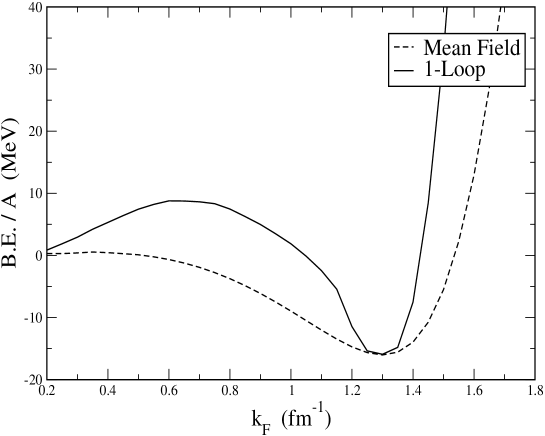
Figure 13: Predictions of a $\sigma$-$\omega$ model for the binding energy per nucleon of symmetric nuclear matter obtained in the mean field and one–boson–loop approximations. The adopted coupling constants are given in Table 1.

8 Conclusions and Perspectives

In this paper we have proposed a functional integral approach to study the static properties of nuclear matter within a fully relativistic scheme, keeping in mind, even if not explicitly considered, the QHD model developed by Serot and Walecka. First, a bosonic effective action has been constructed for a system of interacting nucleons and $\sigma$ mesons. Special attention has been devoted to the formulation of a renormalization procedure for the introduced bosonic effective action. We have then evaluated the resulting partition function through a Semiclassical expansion around the solution given by the stationary phase approximation: this allowed us to express the result in terms of a boson loop expansion. Hartree–dressed nucleons and RPA–dressed bosons have revealed themselves to be the basic elements of this BLE. The suggested scheme has been analyzed at the mean field level and at the one– and two–boson–loop orders. We have presented a thorough exposition of the formal derivation of the binding energy per nucleon, the pressure and the compressibility of nuclear matter up to the second order in the BLE.

Numerical results for the nuclear matter binding energy at the one–boson–loop level have been presented for a realistic, dynamical model including the $\omega$ meson in addition to the $\sigma$. The convergence properties of the BLE have been discussed in this context. A systematic calculation of the static properties of nuclear matter up to the two–boson–loop order and in the $\sigma$-$\omega$ model will be the object of a forthcoming paper, where we shall also deal with the formal derivation of the higher orders of the BLE. The inclusion of the $\omega$ meson is not a prohibitive task from the point of view of the diagrammatic content, since the basic topology of the boson loops (see Figures 11 and 12) is common to any meson field which can contribute to the dynamics. However, since the $\omega^{0}$ component is coupled, in infinite nuclear matter, to the $\sigma$ meson (due to the breaking of the Lorentz invariance induced by the infinite medium) [34], the RPA equations, which deeply intervene in the corrections beyond the mean field, are much more involved that those presented here.

Further, we note that the implementation of the isovector mesons $\rho$ and $\delta\,[f_{0}(980)]$ in our framework does not introduce additional difficulties from a technical point of view. Up to now, however, they have been handled only at the mean field level [27].

It is worth noticing that at the mean field level no pseudoscalar and pseudovector mesons can be coupled to the nucleon density or current, since the average values of pseudoscalar and pseudovector quantities vanish. However, the situation is completely different when boson loops are involved. It is indeed known that the two–pion exchange diagrams, with the possible simultaneous excitation of one or two intermediate nucleons to a $\Delta$, provide a large amount of the nuclear binding. We shall explore this mechanism in the future, but we reasonably expect that a drastic change in the underlying dynamics of QHD will occur and that the gap between QHD and Bonn potential models will be further, and significantly, reduced.

Appendix

In the regularization scheme expressed by Eq. (59) the explicit expression of the scalar density, $\rho_{s}(m)=\rho_{s\,v}(m)+\rho_{sM}(m)$, is given by:

$$\rho_{s\,v}(m) = \frac{m\Lambda^{4}}{2\pi^{2}(m^{2}-\Lambda^{2})}\left\{1+\frac{m^{2}}{m^{2}-\Lambda^{2}}\log\frac{\Lambda^{2}}{m^{2}}\right\}~{},$$

$$\rho_{sM}(m) = \frac{m\Lambda^{4}}{\pi^{2}(m^{2}-\Lambda^{2})^{2}}\left\{k_{F}E_{F}-m^{2}\log\frac{k_{F}+E_{F}}{m}\right\}~{},$$

with the limiting behavior

$$\rho_{s\,v}(m)\mathop{\longrightarrow}_{\Lambda\to\infty}-\frac{m}{2\pi^{2}}\left(\Lambda^{2}-2m^{2}\log\frac{\Lambda}{m}+m^{2}\right)~{}.$$

The quantity $\Pi^{(d)}_{v}(q^{2})$ introduced in Eqs. (78) and (79) reads

$$\Pi^{(d)}_{v}(q^{2})=\frac{\left(4m^{2}-q^{2}\right)^{3/2}\arctan\left(\frac{\displaystyle q}{\displaystyle\sqrt{4m^{2}-q^{2}}}\right)\Lambda^{4}}{2\pi^{2}q(m-\Lambda)^{2}(m+\Lambda)^{2}}$$

$$-\bigl{(}-m^{6}+11q^{2}m^{4}+3\Lambda^{2}m^{4}-7q^{4}m^{2}-3\Lambda^{4}m^{2}+6q^{2}\Lambda^{2}$$

$$+m^{2}+q^{6}+\Lambda^{6}-q^{2}\Lambda^{4}-q^{4}\Lambda^{2}\bigr{)}$$

$$\times\frac{\Lambda^{4}}{4\pi^{2}q^{2}(m^{2}-\Lambda^{2})^{2}\sqrt{m-q-\Lambda}\sqrt{m+q-\Lambda}\sqrt{m-q+\Lambda}\sqrt{m+q+\Lambda}}$$

$$\times\Biggl{[}{\rm arctanh}\left(\frac{m^{2}-q^{2}-\Lambda^{2}}{\sqrt{m-q-\Lambda}\sqrt{m+q-\Lambda}\sqrt{m-q+\Lambda}\sqrt{m+q+\Lambda}}\right)$$

$$-{\rm arctanh}\left(\frac{m^{2}+q^{2}-\Lambda^{2}}{\sqrt{m-q-\Lambda}\sqrt{m+q-\Lambda}\sqrt{m-q+\Lambda}\sqrt{m+q+\Lambda}}\right)\Biggr{]}$$

$$-\frac{\left(m^{4}-6q^{2}m^{2}-2\Lambda^{2}m^{2}+q^{4}+\Lambda^{4}\right)\log\left(\frac{\displaystyle m}{\displaystyle\Lambda}\right)\Lambda^{4}}{4\pi^{2}q^{2}(m^{2}-\Lambda^{2})^{2}}-\frac{\Lambda^{4}}{4\pi^{2}\left(m^{2}-\Lambda^{2}\right)}~{}.$$

In the limit $\Lambda\to\infty$ and within a hard normalization scheme we find

$$\Pi^{(d)}_{v}(m_{\sigma}^{2}) = \frac{1}{2\pi^{2}}\Biggl{\{}\Lambda^{2}-(6m^{2}-m^{2}_{\sigma})\log\frac{\Lambda}{m}$$

$$+\frac{4m^{2}+m^{2}_{\sigma}}{4}+\frac{(4m^{2}-m^{2}_{\sigma})^{\frac{3}{2}}}{m_{\sigma}}\arctan\frac{m_{\sigma}}{\sqrt{4m^{2}-m^{2}_{\sigma}}}\Biggr{\}}~{},$$

and

$$\frac{d\Pi^{(d)}_{v}(q^{2})}{dq^{2}}\Bigm{|}_{q^{2}=m_{\sigma}^{2}} = \frac{1}{2\pi^{2}}\Biggl{\{}-\frac{1}{4}+\frac{2m^{2}}{m_{\sigma}^{2}}$$

$$-\frac{\sqrt{4m^{2}-m_{\sigma}^{2}}(2m^{2}+m_{\sigma}^{2})}{m_{\sigma}^{3}}\arctan\frac{m_{\sigma}}{\sqrt{4m^{2}-m_{\sigma}^{2}}}+\log\frac{\Lambda}{m}\Biggr{\}}~{}.$$

On the contrary, by choosing the renormalization point at $q^{2}=0$ we find

$$\begin{split}\Pi^{(d)}_{v}(0)&=\frac{\Lambda^{4}}{2\pi^{2}}\left\{\frac{3m^{2}+\Lambda^{2}}{(\Lambda^{2}-m^{2})^{2}}-2m^{2}\frac{3\Lambda^{2}+m^{2}}{(\Lambda^{2}-m^{2})^{3}}\log\frac{\Lambda}{m}\right\}\\ &\mathop{\longrightarrow}_{\Lambda\to\infty}\frac{1}{2\pi^{2}}\left\{\Lambda^{2}-6m^{2}\log\frac{\Lambda}{m}+5m^{2}\right\}~{},\end{split}$$

and

$$\begin{split}\frac{d\Pi^{(d)}_{v}(q^{2})}{dq^{2}}\Bigm{|}_{q^{2}=0}&=\Biggl{\{}\frac{-\Lambda^{4}(13\Lambda^{4}-68m^{2}\Lambda^{2}-41m^{4})}{24\pi^{2}(\Lambda^{2}-m^{2})^{4}}\\ &+\frac{\Lambda^{4}(\Lambda^{6}-3m^{2}\Lambda^{4}-12m^{4}\Lambda^{2}-2m^{6}}{2\pi^{2}(\Lambda^{2}-m^{2})^{5}}\log\frac{\Lambda}{m}\Biggr{\}}\\ &\mathop{\longrightarrow}_{\Lambda\to\infty}-\frac{13}{24\pi^{2}}+\frac{1}{2\pi^{2}}\log\frac{\Lambda}{m}~{}.\end{split}$$

For the $\sigma\sigma\sigma$ vertex function of Eq. (81) we have

$$\begin{split}\widetilde{\Gamma}^{(e)}&=\frac{2m\Lambda^{4}\left(m^{2}+2\Lambda^{2}\right)}{\pi^{2}(m-\Lambda)^{3}(m+\Lambda)^{3}}+\frac{m\Lambda^{4}\left(m^{4}+8\Lambda^{2}m^{2}+3\Lambda^{4}\right)}{\pi^{2}(m-\Lambda)^{4}(m+\Lambda)^{4}}\log\frac{\Lambda}{m}\\ &\mathop{\longrightarrow}_{\Lambda\to\infty}-\frac{4m}{\pi^{2}}+\frac{3m}{\pi^{2}}\log\frac{\Lambda}{m}\end{split}$$

and for the $\sigma\sigma\sigma\sigma$ self–coupling of Eq. (82):

$$\begin{split}\widetilde{\Gamma}^{(f)}&=-\frac{\left(7m^{4}+34\Lambda^{2}m^{2}+7\Lambda^{4}\right)\Lambda^{4}}{3\pi^{2}(\Lambda-m)^{4}(m+\Lambda)^{4}}+\frac{\left(m^{2}+\Lambda^{2}\right)\left(m^{4}+14\Lambda^{2}m^{2}+\Lambda^{4}\right)\Lambda^{4}}{\pi^{2}(\Lambda-m)^{5}(m+\Lambda)^{5}}\log\frac{\Lambda}{m}\\ &\mathop{\longrightarrow}_{\Lambda\to\infty}-\frac{7}{3\pi^{2}}+\frac{1}{\pi^{2}}\log\frac{\Lambda}{m}~{}.\end{split}$$

References

• [1] R. Jackiw, Phys. Rev. D 9, 1686 (1974); J. M. Cornwall, R. Jackiw and E. Tomboulis, Phys. Rev. D 10, 2428 (1974).
• [2] J. Iliopoulos, C. Itzykson and A. Martin, Rev. Mod. Phys. 47, 165 (1975).
• [3] J. W. Negele, Rev. Mod. Phys. 54, 813 (1982).
• [4] C. Itzykson and J.-B. Zuber, Quantum Field Theory (McGraw-Hill Book co., Singapore, 1980).
• [5] D. J. Amit, Field Theory, the Renormalization Group, and Critical Phenomena (World Scientific, Singapore, 1984).
• [6] J. W. Negele and H. Orland, Quantum Many Particle Systems (Addison-Wesley, Redwood, 1988).
• [7] B. D. Serot and J. D. Walecka, Adv. Nucl. Phys, 16, 1 (1986); Int. J. Mod. Phys. E 6, 515 (1997).
• [8] S. A. Chin, Annals Phys.  108 (1977) 301.
• [9] R. J. Furnstahl, R. J. Perry and B. D. Serot, Phys. Rev.  C 40, 321 (1989).
• [10] M. Prakash P. J. Ellis and J. I. Kapusta, Phys. Rev. C 45, 2518 (1992).
• [11] R. Friedrich, K. Wehrberger and F. Beck, Phys. Rev. C 46, 188 (1992).
• [12] B. D. Serot and H.-B. Tang, Phys. Rev. C 51, 969 (1992).
• [13] T. D. Lee and G. C. Wick, Phys. Rev. D 9, 2291 (1974).
• [14] R. J. Furnstahl and B. D. Serot, Comments Nucl. Part. Phys. 2, A23 (2000).
• [15] N. Weiss, Phys. Rev. D 27, 899 (1983).
• [16] K. Wehrberger, R. Wittman and B. D. Serot, Phys. Rev. C 42, 2680 (1990).
• [17] W. M. Alberico, R. Cenni, A. Molinari and P. Saracco, Ann. of Phys. 174, 131 (1987).
• [18] R. Cenni and P. Saracco, Nucl. Phys. A487, 279 (1988).
• [19] W. M. Alberico, R. Cenni, A. Molinari and P. Saracco, Phys. Rev. Lett. 65, 1845 (1990).
• [20] R. Cenni and P. Saracco, Phys. Rev. C 50, 1851 (1994).
• [21] R. Cenni, F. Conte and P. Saracco, Nucl. Phys A 623, 391 (1997).
• [22] P. Amore, R. Cenni and P. Saracco, Nuovo Cim. A 112, 1015 (1999).
• [23] W. M. Alberico, A. De Pace, G. Garbarino and R. Cenni, Nucl. Phys. A 668, 113 (2000).
• [24] R. Machleidt, K. Holinde and Ch. Elster, Phys. Rep. 149, 1 (1987).
• [25] H. Ruegg and M. Ruiz-Altaba, Int. J. Mod. Phys. A 19, 3265 (2004).
• [26] S. Kubis and M. Kutschera, Phys. Lett. B 399, 191 (1997).
• [27] B. Liu, V. Greco, V. Baran, M. Colonna and M. Di Toro, Phys. Rev. C 65, 045201 (2002).
• [28] R. Cenni, F. Conte, A. Cornacchia and P. Saracco, Riv. Nuovo Cim. 15 N 12, 1 (1992).
• [29] W. M. Alberico, R. Cenni, A. Molinari and P. Saracco, Phys. Rev., C 38, 2389 (1988).
• [30] M. B. Barbaro, R. Cenni and M. R. Quaglia, Eur. Phys. J. A 25, 299 (2005).
• [31] J. Collins, Renormalization (Cambridge University Press, Cambridge, 1984).
• [32] R. J. Furnstahl, B. D. Serot and H.-B. Tang, Nucl. Phys. A 618, 446 (1997).
• [33] A. L. Fetter and J. D. Walecka, Quantum Theory of Many–Particle Systems (McGraw–Hill, New York, 1971).
• [34] A. K. Dutt-Mazumder, Nucl. Phys. A 713, 119 (2003).