A Refined Numerical Result on the First Excitation Energy in the Two-Level Pairing Model

Abstract

The first excitation energy in the two-level pairing model is investigated in terms of the equilibrium and the small fluctuation around it. The basic idea is an extension of results presented in a previous paper by the present authors. In this investigation, the result obtained in the previous paper plays a central role: At the limit of the weak and the strong interaction strength, the results are in good agreement with the exact one. The former and the latter are calculated in the framework of the $su(2)\otimes su(1,1)$- and the $su(2)\otimes su(2)$-coherent state, respectively. On the basis of the above conclusion, the intermediate region for the interaction strength is described in terms of the idea of the interpolation and it is shown that the agreement of the result with the exact one is quite good.

The description of the first excited state in the two-level pairing model for the closed shell system has been regarded as a basic, but a modest problem in many-body physics. For example, the recent investigations can be found in Ref. 1. Following this quiet stream, recently, the present authors have considered this problem from tow slightly different viewpoints. One was reported in Ref.2 and the other in Refs.3 and 4. Especially, in Ref.4 (referred to as (I)), the ground-state and the first excitation energy are calculated in the framework of three different coherent states which consisit of four kinds of boson operators. In (I), they are called (i) the $su(2)\otimes su(1,1)$-, (ii) the $su(1,1)\otimes su(1,1)$- and (iii) the $su(2)\otimes su(2)$-coherent states. The picture adopted in (I) is based on the equilibrium and the fluctuation around it and the equilibrium state is described by a coherent state. Therefore, we obtain three different equilibrium states. Roughly speaking, for the first excited energy, in the region of weak strength of the pairing interaction, the state (i) gives rather good result. But, in the region of strong strength, the state (iii) gives good result. Compared with the above two states, it seems to us that the state (ii) gives a slightly worse result. Of course, the above rough summary is based on the comparison with the exact result.

Before entering the central parts of this paper, we mention our basic viewpoint. We pay attention to the relation appearing in the appendix (B) of (I), i.e., (I$\cdot$B$\cdot$1). This relation demonstrates that, if we solve our system exactly in the quantum mechanical framework, the result does not depend on the choice of the function $g({\hat{K}})$. The part of the Hamiltonian, ${\hat{H}}_{1}$, is recast into

$${\hat{H}}_{1} = -G\left[\sqrt{g({\hat{K}})}\cdot\sqrt{\hbar}{\hat{c}}^{*}\sqrt{2T+{\hat{K}}}\sqrt{2M-{\hat{K}}}\sqrt{2L-{\hat{K}}}\cdot\left(\sqrt{g({\hat{K}}+\hbar)}\right)^{-1}+{\rm h.c.}\right]$$ (1)

$$= -G\left[\sqrt{\hbar}{\hat{c}}^{*}\sqrt{2T+{\hat{K}}}\sqrt{2M-{\hat{K}}}\sqrt{2L-{\hat{K}}}+{\rm h.c.}\right]\ ,$$

where h.c. means the Hermitian conjugation. It should be noted that the relation (1) holds for any form of $g({\hat{K}})$ if it can be defined. On the other hand, the $c$-number replacement gives the form

$${H}_{1} = -G\left[\sqrt{g(K)}\cdot\sqrt{\hbar}{c}^{*}\sqrt{2T+{K}}\sqrt{2M-{K}}\sqrt{2L-{K}}\cdot\left(\sqrt{g(K+\hbar)}\right)^{-1}+{\rm c.c.}\right]$$ (2)

$$= -G\left[\sqrt{\hbar}{c}^{*}\sqrt{2T+{K}}\sqrt{2M-{K}}\sqrt{2L-{K}}\cdot\sqrt{g(K)\cdot g(K+\hbar)^{-1}}+{\rm c.c.}\right]\ ,$$

where c.c. means the complex conjugation. The relation (2) tells us that the classical solution based on the relation (2) depends on the choice of $g(K)$. The above means that the classical counterpart under the $c$-number replacement cannot be fixed uniquely, that is, there exist infinite possibilities for the classical solutions which should correspond to the unique quantum mechanical solution. However, we must note that we determine the equilibrium by a classical solution and the fluctuation is given in the lowest order for classical and quantum mechanical framework. Therefore, the result depends on the form of $g(K)$, and the principle, with the aid of which $g(K)$ is fixed, is required. In (I), we investigated three possibilities which come from three forms of the coherent state.

As was demonstrated in (I), the key to obtain a good result is to choose the function $f({\hat{K}})$ related to $g({\hat{K}})$ and defined through the form (I$\cdot$B$\cdot$2), i.e., $f(K)$. The three cases are shown in the relation (I$\cdot$4$\cdot$4) and in Fig.(I$\cdot$2), the different behaviors are explicitly presented. Here, “good result” means the agreement with the exact one. From this figure, we learn that if we succeed in finding the function $f(K)$, which satisfies the following condition, the good result may be expected: For a small value of $K$, $f(K)$ shows the behavior shown in Fig.(I$\cdot$2a) and in the region $K{\stackrel{{\scriptstyle<}}{{\sim}}}\Omega/2$, the behavior of $f(K)$ should be as shown in Fig.(I$\cdot$2c). In this paper, we present some candidates for $f(K)$ which show the above behavior under the idea of an interpolation.

Instead of $f(K)$, we investigate the function $\mu(K)$ defined as

$$f(K)=2G\mu(K)\ .$$ (3)

In the case of the states (i) and (iii), $\mu(K)$ can be expressed in the form

$$\mu_{\rm i}(K)=\sqrt{K(K+1)}(\Omega-K)\ ,$$ (4)

$$\mu_{\rm iii}(K)=K(\Omega-K)\ .$$ (5)

Hereafter, we use the unit $\hbar=1$. The function $\mu_{\rm i}(K)$ can be expanded in the form

$$\mu_{\rm i}(K)=\sqrt{K}\left(\Omega+(\Omega/2-1)K+\cdots\right)\ .$$ (6)

On the other hand, $\mu_{\rm iii}(K)$ can be rewritten as

$$\mu_{\rm iii}(K)=(\Omega/2)^{2}+0\times(\Omega/2-K)-(\Omega/2-K)^{2}\ .$$ (7)

Therefore, the leading terms for $\mu_{\rm i}(K)$ near $K\sim 0$ and for $\mu_{\rm iii}(K)$ near $K\sim\Omega/2$ are as follows:

$$\mu_{\rm i}(K)=\sqrt{K}\Omega\ ,$$ (8)

$$\mu_{\rm iii}(K)=(\Omega/2)^{2}+0\times(\Omega/2-K)\ .$$ (9)

Our problem is to find an explicit form for $\mu(K)$ which reduces to the forms (8) and (9) for $K\sim 0$ and $K\sim\Omega/2$, respectively, in the framework of the idea of an interpolation.

First, let us search $\mu(K)$ in the form

$$\mu(K)=\sqrt{K(K+n)}A(B-K)\ .$$ (10)

Here, $n$, $A$ and $B$ denote parameters to be determined as functions of $\Omega$. The function $\mu(K)$ is expanded in the form

$$\mu(K)=\sqrt{K}\left[\sqrt{n}AB+A(B/2\sqrt{n}-\sqrt{n})K+\cdots\right]\ .$$ (11a)

Also, in terms of $$(\Omega/2-K) \mu(K)$$, is expressed as

$$\mu(K) = \sqrt{\Omega(\Omega+2n)}/2\cdot A(B-\Omega/2)$$

$$+\sqrt{\Omega(\Omega+2n)}/2\cdot A\left[1-(B-\Omega/2)\frac{2(\Omega+n)}{\Omega(\Omega+2n)}\right](\Omega/2-K)$$

$$-\frac{A}{\sqrt{\Omega(\Omega+2n)}}\left[(\Omega+n)+(B-\Omega/2)\frac{n^{2}}{\Omega(\Omega+2n)}\right](\Omega/2-K)^{2}+\cdots\ .$$

Comparison of the forms (11a) and (LABEL:11b) with the asymptotic forms (8) and (9) gives us the relation

$$\sqrt{n}AB=\Omega\ ,$$ (12a)

$$\sqrt{\Omega(\Omega+2n)}A(B-\Omega/2)=(\Omega/2)^{2}\ ,$$ (12b)

$$1-(B-\Omega/2)\cdot\frac{2(\Omega+n)}{\Omega(\Omega+2n)}=0\ .$$ (12c)

The relations (12b) and (12c) lead to

$$A=\frac{\sqrt{\Omega}(\Omega+n)}{\left(\sqrt{\Omega+2n}\right)^{3}}\ ,\qquad B=\Omega\left(\frac{\Omega+3n/2}{\Omega+n}\right)\ .$$ (13)

Substituting the form (13) into the relation (12a), we have

$$n=\frac{(\Omega+2n)^{3}}{\Omega(\Omega+3n/2)^{2}}\ .$$ (14)

By solving the relation (14), we can express $n$ in terms of $\Omega$ and the relation (13) gives $A$ and $B$ expressed in terms of $\Omega$. In the case $\Omega=5$, for which we show the numerical results in figures, we have

$$n=2.8441\ ,\qquad A=0.5020\ ,\qquad B=5.9064\ .$$ (15)

Next, we investigate a possible improvement of the form (10) with the relations (13) and (14). We set up the following form:

$$\mu(K)=\sqrt{K(K+n)}A(B-K)\cdot\rho(K)\ .$$ (16)

If $\rho(K)=1$ in the region $0\leq K\leq\Omega/2$, the improvement is not achieved. If we intend to keep the forms (13) and (14) in the improvement, $\rho(K)$ should satisfy

$$\rho(0)=\rho(\Omega/2)=1\ ,\qquad\rho^{\prime}(\Omega/2)=0\ .$$ (17)

As a possible candidate, we can choose the form

$$\rho(K)=\sqrt{\frac{1+C\cdot(\Omega/2)^{-4}(\Omega/2-K)^{4}}{1+C\cdot(\Omega/2)^{-2}(\Omega/2-K)^{2}}}\ .$$ (18)

Here, $C$ denotes a new parameter to be determined as a function of $\Omega$. From the comparison with the exact result, we can see that the large value of $K$ $(\sim\Omega/2)$ should be improved. Then, we expand $\rho(K)$ in terms of $(\Omega/2-K)$:

$$\rho(K)=1-(C/2)\cdot(\Omega/2)^{-2}(\Omega/2-K)^{2}+\cdots\ .$$ (19)

Then, the expression (LABEL:11b) should be improved in the form

the term improved from the third term in the expansion (LABEL:11b) (20)

$$= -\biggl{[}\frac{A}{\sqrt{\Omega(\Omega+2n)}}\left((\Omega+n)+(B-\Omega/2)\frac{n^{2}}{\Omega(\Omega+2n)}\right)$$

$$+\sqrt{\Omega(\Omega+2n)}/2\cdot A(B-\Omega/2)\cdot(C/2)(\Omega/2)^{-2}\biggl{]}(\Omega/2-K)^{2}\ .$$

By putting the form (20) equal to the third terms of the relation (7), we obtain

$$\frac{A}{\sqrt{\Omega(\Omega+2n)}}\left[(\Omega+n)+(B-\Omega/2)\frac{n^{2}}{\Omega(\Omega+2n)}\right]$$

$$+\sqrt{\Omega(\Omega+2n)}/2\cdot A(B-\Omega/2)\cdot(C/2)(\Omega/2)^{-2}=1\ .$$ (21)

By substituting the result (13) for $A$ and $B$ into the form (A Refined Numerical Result on the First Excitation Energy in the Two-Level Pairing Model), $C$ is determined as

$$C=\frac{2n(\Omega+5n/4)}{(\Omega+2n)^{2}}\ .$$ (22)

The case $\Omega=5$ gives us

$$C=0.4260\ .$$ (23)

As is clear from the relation (I$\cdot$B$\cdot$4), it is also an important task for the present description to obtain the function $g(K)$ defined through the relation

$$\mu(K)=\sqrt{K(K+1)}(\Omega-K)\sqrt{g(K)\cdot g(K+1)^{-1}}\ .$$ (24)

In the present case, we have

$$g(K)\cdot g(K+1)^{-1}=A^{2}\left(\frac{K+n}{K+1}\right)\left(\frac{B-K}{\Omega-K}\right)\cdot\xi(\Omega,K)\ .$$ (25)

For the expression (10), we have

$$\xi_{1}(\Omega,K)=1\ .$$ (26)

For the expression (16) with the candidate (18), $\xi_{2}(\Omega,K)$ is given as

$$\xi_{2}(\Omega,K) = (\Omega/2)^{-2}\left[(\Omega/2)\left\{(1+1/\sqrt{2}\sqrt[4]{C})+i\cdot 1/\sqrt{2}\sqrt[4]{C}\right\}-K\right]$$ (27)

$$\qquad\qquad\times\left[(\Omega/2)\left\{(1-1/\sqrt{2}\sqrt[4]{C})+i\cdot 1/\sqrt{2}\sqrt[4]{C}\right\}-K\right]$$

$$\qquad\qquad\times\left[(\Omega/2)(1+i/\sqrt{C})-K\right]^{-1}$$

$$\qquad\qquad\times\left[{\rm c.c.}\right]\ .$$

The notation $[{\rm c.c}]$ denotes the complex conjugate of all the previous terms. Hereafter, we distinguish the two cases by the indeces 1 and 2. For finding the functions $g_{1}(K)$ and $g_{2}(K)$, the following formulae are useful:

$$(i) \ {\rm if}\quad h(K)\cdot h(K+1)^{-1}=\alpha\ ,\qquad h(K)=\beta\alpha^{-K}\ ,$$ (28a)

$$(ii) \ {\rm if}\quad h(K)\cdot h(K+1)^{-1}=\alpha-K\ ,\qquad h(K)=\beta\Gamma(\alpha+1-K)\ ,$$ (28b)

$$(iii) \ {\rm if}\quad h(K)\cdot h(K+1)^{-1}=\alpha+K\ ,\qquad h(K)=\beta\Gamma(\alpha+K)^{-1}\ .$$ (28c)

Here, $\alpha$ and $\beta$ do not depend on $K$ and $\Gamma(z)$ denotes the gamma-function. As can be seen in the relation (I$\cdot$B$\cdot$4), we need only the form $g^{\prime}(K_{0})/g(K_{0})$, and then, it may be enough to put $\beta=1$ for the formula (28). With the use of the formula (28), we obtain the following relations for $g(K)$:

$$g_{1}(K) = A^{-2K}\cdot\Gamma(1+K)\cdot\Gamma(n+K)^{-1}\cdot\left[\Gamma(B+1-K)\cdot\Gamma(\Omega+1-K)^{-1}\right]^{2}\ ,\qquad$$ (29)

$$g_{2}(K) = g_{1}(K)(\Omega/2)^{2K}$$ (30)

$$\times\Gamma((\Omega/2)\{(1+1/\sqrt{2}\sqrt[4]{C})+i\cdot 1/\sqrt{2}\sqrt[4]{C}\}+1-K)$$

$$\times\Gamma((\Omega/2)\{(1-1/\sqrt{2}\sqrt[4]{C})+i\cdot 1/\sqrt{2}\sqrt[4]{C}\}+1-K)$$

$$\times\left[\Gamma((\Omega/2)(1+i/\sqrt{C})+1-K)\right]^{-1}$$

$$\times\left[{\rm c.c.}\right]\ .$$

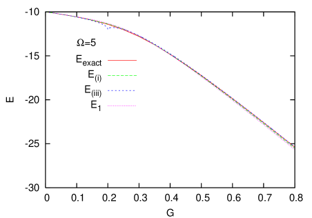
Figure 1: The energies obtained by the use of the various states are depicted as a function of $G$. Here, $E_{\rm(i)}$ and $E_{\rm(iii)}$ denote the derived energies by using of $\mu_{\rm i}$ and $\mu_{\rm iii}$ in Eqs.(4) and (5), respectively, and $E_{1}$ denotes the energy by using of $\mu(K)$ in (10) with (13)$\sim$(15), where $\Omega=5$. Here, $E_{\rm exact}$ shows the exact eigenvalue of the Hamiltonian.

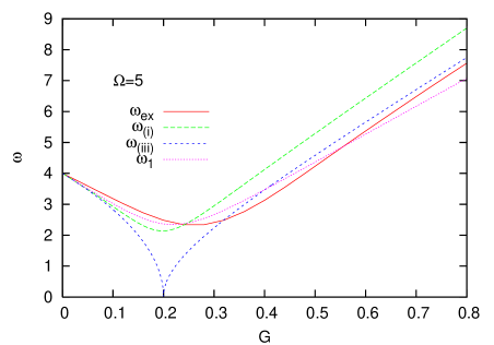
Figure 2: The frequencies are depicted as a function of $G$. Here, $\omega_{\rm(i)}$ and $\omega_{\rm(iii)}$ denote the derived frequencies by using of $\mu_{\rm i}$ and $\mu_{\rm iii}$ in Eqs.(4) and (5), respectively, and $\omega_{1}$ denotes the frequency by using of $\mu(K)$ in (10) with (13)$\sim$(15), where $\Omega=5$. Here, $\omega_{\rm ex}$ shows the exact result.

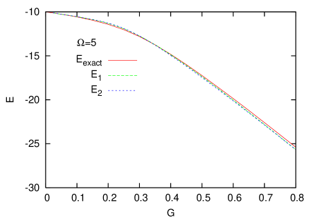
Figure 3: The energies obtained by the use of the new $\mu(K)$ are depicted as a function of $G$. Here, $E_{1}$ and $E_{2}$ denote the derived energies by using of $\mu(K)$ in (10) and (16) with (18), respectively, and $E_{\rm exact}$ shows the exact eigenvalue of the Hamiltonian. Here, $\Omega=5$.

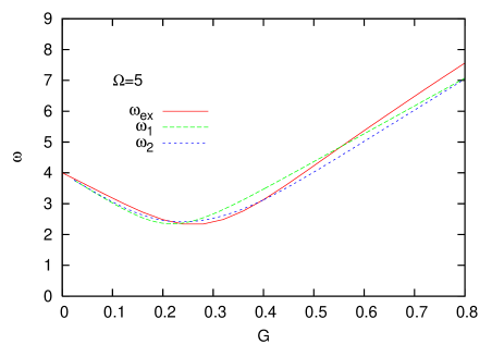
Figure 4: The frequencies obtained by the use of the new $\mu(K)$ are depicted as a function of $G$. Here, $\omega_{1}$ and $\omega_{2}$ denote the derived frequencies by using of $\mu(K)$ in (10) and (16) with (18), respectively, and $\omega_{\rm ex}$ shows the exact result. Here, $\Omega=5$.

In Fig.1, the derived energies of equilibrium are compared with the exact ground state energy $E_{\rm exact}$. Here, $E_{\rm(i)}$ and $E_{\rm(iii)}$ denote the energies obtained by using $\mu_{\rm i}$ in Eq.(4) and $\mu_{\rm iii}$ in Eq.(5), respectively, and $E_{1}$ denotes the energy newly obtained by using the $\mu(K)$ in Eq.(10). Also, in Fig.2, the derived first excitation energies or frequencies of small oscillations around the equilibrium are compared with the exact first excitation energy $\omega_{\rm ex}$. Here, $\omega_{\rm(i)}$ and $\omega_{\rm(iii)}$ denote the first excitation energies obtained by using $\mu_{\rm i}$ in Eq.(4) and $\mu_{\rm iii}$ in Eq.(5), respectively, and $\omega_{1}$ denotes the first excitation energy newly obtained by using the $\mu(K)$ in Eq.(10). The energy of equilibrium is not so refined except for the region presenting a dip structure in $E_{\rm(iii)}$. However, the frequency $\omega_{1}$ is obviously refined. In the region of the weak interaction strength $G$, the behavior of $\omega_{1}$ is similar to $\omega_{\rm(i)}$ by using the $su(2)\otimes su(1,1)$-coherent state as is expected. On the other hand, in the region of the strong interaction strength, the behavior of $\omega_{1}$ is similar to $\omega_{\rm(iii)}$ by using the $su(2)\otimes su(2)$-coherent state. As a result, the obtained result is better in comparison with the exact first excitation energy.

Further, we have improved the function $\mu(K)$ by introducing the function $\rho(K)$ in Eq.(10). Here, we attach the suffix 2 to the quantities derived by using the function $\rho(K)$ in Eqs.(18). In Fig.3, the equilibrium energies are depicted in order to compare them with the exact ground state energy and $E_{1}$ corresponding to the case $\rho(K)=1$. The refinement by using the newly introduced function $\rho(K)$ is also seen in the frequency $\omega$ in Fig.4 transparently. In the weak interaction strength region, the refinement is further obtained in comparison with $\omega_{1}$ with $\rho(K)=1$. In the strong intearction strength region, the obtained frequency runs almost parallel to the exact one as a function of $G$. In addition to the above-mentioned refinement, even in the intermediate region of the interaction strength, the behavior is similar to the exact result and a fairly good result is obtained.

In conclusion, the refined results for the first excitation energy around the equilibrium given by the coherent states have been obtained in the formulation of the idea in which the function $g(K)$ reveals the similar asymptotic behavior to those of the $su(2)\otimes su(1,1)$- and the $su(2)\otimes su(2)$-coherent states. The results shown in this paper teaches us that, following the increase of the interaction strength, the $su(2)\otimes su(1,1)$-symmetry changes gradually to the $su(2)\otimes su(2)$-symmetry. An interesting future problem is to investigate which coherent state can describe the above-mentioned change of the symmetry.

References

[1]
M. Samabataro and N. Dinh Dang, Phys. Rev. C 59 (1999), 1422.
A. Rabhi, R. Bennaceur, G. Chanfray and P. Schuck, Phys. Rev. C 66
(2002), 064315.
N. Dinh Dang, Euro. Phys. J. A 16 (2003), 181.
A Rabhi, Eur. Phys. J. A 20 (2004), 277.
[2]
M. Yamamura, C. Providência, J. da Providência, F. Cordeiro and Y. Tsue,
J. of Phys. A: Math. Gen. 39 (2006), 11193.
[3]
C. Providência, J. da Providência, Y. Tsue and M. Yamamura,
Prog. Theor. Phys. 115 (2006), 739; 759.
[4]
Y. Tsue, C. Providência, J. da Providência and M. Yamamura,
submitted to Prog. Theor. Phys. (nucl-th/0610074)