Critical point symmetries in boson-fermion systems. The case of shape transition in odd nuclei in a multi-orbit model

Abstract

We investigate phase transitions in boson-fermion systems. We propose an analytically solvable model (E(5/12)) to describe odd nuclei at the critical point in the transition from the spherical to $\gamma$-unstable behaviour. In the model, a boson core described within the Bohr Hamiltonian interacts with an unpaired particle assumed to be moving in the three single particle orbitals j=1/2,3/2,5/2. Energy spectra and electromagnetic transitions at the critical point compare well with the results obtained within the Interacting Boson Fermion Model, with a boson-fermion Hamiltonian that describes the same physical situation.

The occurrence of shape transitional behaviour characterizes both even-even and odd nuclei. Because of the further complexity embodied in the description of the coupling of the odd particle to the even core, formalisms describing phase transitions have been initially mainly devised for even systems. Only recently the study of phase transitions in odd-nuclei has been revitalized. The first case considered by IachelloE54 ; cam ; caprio has been the case of a j=3/2 fermion coupled to a boson core that undergoes a transition from spherical to $\gamma$-unstable. At the critical point, an elegant analytic solution, called E(5/4), has been obtained starting from the Bohr Hamiltonian. The possible occurrence of this symmetry in ¹³⁵Ba has been recently suggested135ba . However, the restriction of the fermion space to a single-j orbit makes difficult the identification of a particular nucleus as critical.

In this letter we consider the richer case of a collective core coupled to a particle moving in the j=1/2, 3/2 and 5/2 single-particle orbits, with the boson part undergoing a transition from sphericity to deformed $\gamma$-instability. This situation is likely to occur in the mass region around A=190, for example in odd-neutron Pt where the relevant active orbitals around the Fermi surface are the $3p_{1/2},3p_{3/2}$ and $2f_{5/2}$, in odd-proton Ir isotopes with active orbits $2d_{5/2},2d_{3/2}$ and $3s_{1/2}$, and also in the region around A=130, in odd-neutron Ba isotopes with relevant orbits $2d_{5/2},2d_{3/2}$ and $3s_{1/2}$, just to cite a few of them. At the critical point we extend the E(5/4) model to the multi-j case, obtaining a new analytic solution, which we will call E(5/12). Knowing the analytic form of the eigenfunctions, it is then easy to calculate spectroscopic observables, such as electromagnetic transition probabilities. To check the validity of the model, we will also present more microscopic calculations based on the Interacting Boson Fermion ModelIVI91 , with a choice of the boson-fermion Hamiltonian that describes the same physical situation. We will show that the E(5/12) and IBFM models give comparable behaviours.

We will then consider the coupling of a collective core, described within the quadrupole collective Bohr Hamiltonian, with an odd particle moving in the 1/2,3/2,5/2 orbitals. One can use the separation of the single-particle angular momentum into a pseudo-spin and pseudo-orbital angular momentum (0 and 2) and assume no coupling due to the pseudo-spin. The pseudo-orbital part transforms as the representations ($\tau_{1}^{F},0$) of $O^{F}(5)$, with $\tau_{1}^{F}$ being either 0 or 1U6/12 . One can therefore use a model Hamiltonian of the form

$$H= - \frac{\hbar^{2}}{2B}\left[\frac{1}{\beta^{4}}\frac{\partial}{\partial\beta}\beta^{4}\frac{\partial}{\partial\beta}+\frac{1}{\beta^{2}\sin{3\gamma}}\frac{\partial}{\partial\gamma}\sin{3\gamma}\frac{\partial}{\partial\gamma}-\frac{1}{4\beta^{4}}\sum_{\kappa}\frac{Q^{2}_{\kappa}}{\sin^{2}{\left(\gamma-\frac{2}{3}\pi\kappa\right)}}\right]$$

$$+ u(\beta)+k~{}g(\beta)[2\hat{\mathcal{L}}_{B}\circ\hat{\mathcal{L}}_{F}]+k^{\prime}~{}g(\beta)\hat{\mathcal{L}}_{F}^{2},$$

with

$$u(\beta)=0,\beta<\beta_{w};~{}u(\beta)=\infty,\beta\geq\beta_{w};~{}g(\beta)=\frac{\hbar^{2}}{2B\beta^{2}}~{},$$ (2)

where $\hat{\mathcal{L}}_{B}$ and $\hat{\mathcal{L}}_{F}$ are the five-dimensional boson and fermion orbital angular momenta, and the dot $\circ$ indicates the five-dimensional scalar product. This Hamiltonian is the generalization of the Hamiltonian used in the E(5/4) model. It should be noted that the last term was not included in E(5/4). In that case a single-j was treated and, consequently, a single $O_{F}(5)$ representation was involved. For the E(5/12) multi-j case two $O_{F}(5)$ representations are present and the last term in (LABEL:Hbohr) is needed in order to include the energy difference between $j=1/2$ and $j=3/2,5/2$ single particle orbits. The choice of an infinite square well in the $\beta$ variable should mimic the actual situation at the critical point of the transition from the spherical situation (potential with a minimum in $\beta$=0) to the deformed $\gamma$-instability (potential with a minimum for a finite value of $\beta$). In this case, since the group characterizing the core transition is the Euclidean one in five dimensions E(5) and the algebra for the fermion space is U(12), we will name the model as E(5/12).

With this choice the total wave function can be factorized in the form

$$\Psi~{}=~{}F(\beta)~{}[\Phi(\gamma,\theta_{i},\eta_{orb})\otimes\chi(\eta_{spin})]^{(J_{BF})}~{},$$ (3)

where $\eta_{orb}$ and $\eta_{spin}$ represent the particle coordinates associated with the pseudo-orbital and the pseudo-spin spaces. The wave function $\Phi$ is characterized by good quantum numbers $(\tau_{1},\tau_{2},\tau_{1}^{B},\tau_{1}^{F},L_{BF},M_{L})$ and is given by

$$\Phi_{(\tau_{1},\tau_{2}),\tau_{1}^{B},\tau_{1}^{F},L_{BF},M_{L}}(\gamma,\theta_{i},\eta_{orb})~{} = ~{}\sum_{{\ell}_{B},m_{{\ell}_{B}},{\ell}_{F},m_{{\ell}_{F}}}\left\langle\begin{array}[]{llll}(\tau_{1}^{B},0)&(\tau_{1}^{F},0)&|&(\tau_{1},\tau_{2})\\ ~{}~{}{\ell}_{B}&~{}~{}{\ell}_{F}&|&~{}~{}L_{BF}\end{array}\right\rangle\left\langle\begin{array}[]{llll}{\ell}_{B}&{\ell}_{F}&|&L_{BF}\\ m_{{\ell}_{B}}&m_{{\ell}_{F}}&|&M_{L}\end{array}\right\rangle$$ (8)

$$\times ~{}\phi_{(\tau_{1}^{B},0),{\ell}_{B},m_{{\ell}_{B}}}(\gamma,\theta_{i})~{}X_{(\tau_{1}^{F},0),{\ell}_{F},m_{{\ell}_{F}}}(\eta_{orb})~{}.$$ (9)

The function $X(\eta_{orb})$ describes the five-dimensional pseudo-orbital part, while $\chi(\eta_{spin})$ is the pseudo-spin wave function, which does not contribute to the energy. The equation for $F(\beta)$ then acquires the familiar form

$$\left[-\frac{\hbar^{2}}{2B}\frac{1}{\beta^{4}}\frac{\partial}{\partial\beta}\beta^{4}\frac{\partial}{\partial\beta}+\frac{\hbar^{2}}{2B}\frac{\Lambda}{\beta^{2}}+u(\beta)\right]F(\beta)~{}=~{}EF(\beta)~{},$$ (10)

with

$$\Lambda =\tau_{1}^{B}(\tau_{1}^{B}+3)+k\left[\tau_{1}(\tau_{1}+3)+\tau_{2}(\tau_{2}+1)\right.$$ (11)

$$- \left.\tau_{1}^{B}(\tau_{1}^{B}+3)-\tau_{1}^{F}(\tau_{1}^{F}+3)\right]+k^{\prime}\tau_{1}^{F}(\tau_{1}^{F}+3).$$

The solutions of this equation, as in the case of the E(5/4) model, are given in terms of Bessel functions of order $\nu=\sqrt{\Lambda+9/4}$, in the form

$$F_{\xi,\{(\tau_{1},\tau_{2}),\tau_{1}^{B},\tau_{1}^{F}\}}(\beta)~{}=~{}c_{\xi,\{(\tau_{1},\tau_{2}),\tau_{1}^{B},\tau_{1}^{F}\}}$$

$$\times\beta^{-3/2}J_{\nu}(x_{\xi,\{(\tau_{1},\tau_{2}),\tau_{1}^{B},\tau_{1}^{F}\}}\beta/\beta_{w})~{},$$ (12)

where $c_{\xi,\{(\tau_{1},\tau_{2}),\tau_{1}^{B},\tau_{1}^{F}\}}$ is a normalization constant and $x_{\xi,\{(\tau_{1},\tau_{2}),\tau_{1}^{B},\tau_{1}^{F}\}}$ the $\xi$-th zero of $J_{\nu}(z)$. The corresponding eigenvalues are given as

$$E_{\xi,\{(\tau_{1},\tau_{2}),\tau_{1}^{B},\tau_{1}^{F}\}}~{}=~{}\frac{\hbar^{2}}{2B}\left(\frac{x_{\xi,\{(\tau_{1},\tau_{2}),\tau_{1}^{B},\tau_{1}^{F}\}}}{\beta_{w}}\right)^{2}.$$ (13)

The corresponding spectrum is given in the upper frame of Fig. 1 for the choice of the parameters $k=-1/4$ and $k^{\prime}=5/2$. Each state is characterized by the $\xi,\tau_{1}^{B},\tau_{1}^{F}(\tau_{1},\tau_{2})$ quantum numbers and arranged in bands according to the counting quantum number $\xi$. The factorization of the pseudo-spin part give rise to repeated level couplets. Most of the states are therefore degenerate, starting from the first excited 3/2-5/2 doublet. The values of the angular momenta (twice) for each degenerate state characterized by the $O^{BF}(5)$ boson-fermion $(\tau_{1},\tau_{2})$ labels are given in the lowest inset panel. The lowest band with $\xi=1$ comes from the coupling of the boson states $(\tau_{1}^{B},0)$ with the fermion states $(\tau_{1}^{F}=0,0)$. It is worth mentioning that all these states with $\tau_{1}^{F}$=0 have precisely the same energies as the states in the even E(5) model. The set of three bands associated to the first excited $\xi=1$ structure comes from the coupling of $(\tau_{1}^{B},0)$ with $(\tau_{1}^{F}=1,0)$ which produces states $(\tau_{1},\tau_{2})$ of the full boson-fermion system labelled as $(\tau_{1}^{B}+1,0)$, $(\tau_{1}^{B},1)$ and $(\tau_{1}^{B}-1,0)$U6/12 . In addition to these $\xi=1$ bands, excited $\xi=2,3,\dots$ structures appear.

Figure 1: Upper frame: Energy levels in the odd system at the E(5/12) critical point (normalized to the energy of the first excited state). Each (degenerate) state is characterized by the $\xi,\tau_{1}^{B},\tau_{1}^{F},(\tau_{1},\tau_{2})$ quantum numbers. The values $k=-1/4,k^{\prime}=5/2$ have been used in the Hamiltonian (LABEL:Hbohr). The values of (twice) the angular momenta for each degenerate state can be extracted from the inset in the lowest panel. Some selected values of $B(E2)$’s, corresponding to the transitions between the highest spins of initial and final multiplets, are given in the figure (the B(E2) associated with the lowest 5/2-1/2 transition is normalized to 100). Lower frame: Energy levels in the odd system within the IBFM Hamiltonian (18) at the critical point. A number of bosons $N=7$ has been assumed. The values of $k$ and $k^{\prime}$ are the same as in the E(5/12) Hamiltonian. For the BE(2)’s, see the upper frame.

We can now calculate quadrupole transitions. In this case only the collective part of the quadrupole transition operator has been used, as in Refs. E54 ; cam ; caprio . The calculation reduces to a single numerical integral over the $\beta$ variable. In Fig. 1 we have chosen to represent the B(E2)’s between the highest spins of initial and final multiplets (the B(E2) associated with the lowest 5/2-1/2 transition is normalized to 100), since most levels are multiply degenerate. Note that states with different $\tau_{1}^{F}$ are not connected between them by E2 transitions.

To check the validity of the model we can describe a similar physical situation within the framework of the Interacting Boson Fermion Model (IBFM)IVI91 , where the coupling of a single fermion to the even-even boson core is described by the Hamiltonian

$$H~{}=~{}H_{B}+H_{F}+V_{BF}~{},$$ (14)

where the term $V_{BF}$ couples the boson and fermion degrees of freedom. We remind that critical point symmetries, as E(5), X(5) or E(5/4), although inspired by models with interacting bosons, can only be approximately obtained within these models. However the comparison with the IBM and IBFM turned out to be useful, e.g. in the case of the E(5) and E(5/4) symmetries, for a better understanding of the characteristics of these modelsbeta4 ; odd ; odd2 . In these cases, the Hamiltonian used for the bosonic part was a parametrized one, that produces a transition between spherical and $\gamma$-unstable shapes, of the form

$$H_{B}=x\hat{n}_{d}-((1-x)/N)~{}\hat{Q}_{B}\cdot\hat{Q}_{B}~{},$$ (15)

where the operators in the Hamiltonian are given by $\hat{n}_{d}=\sum_{\mu}d^{\dagger}_{\mu}d_{\mu}$ and $\hat{Q}_{B}=(s^{\dagger}\times\tilde{d}+d^{\dagger}\times\tilde{s})^{(2)}$, and $N$ is the total number of bosons. This Hamiltonian can be recast into the form

$$H_{B}=xC_{1}(U^{B}(5))-\frac{1-x}{2N}\left[C_{2}(O^{B}(6))-C_{2}(O^{B}(5))\right],$$ (16)

where $C_{1}(U^{B}(5))$ is the linear Casimir operator of the $U^{B}(5)$ algebra, while $C_{2}(O^{B}(6))$ and $C_{2}(O^{B}(5))$ are the quadratic Casimir operators of the $O^{B}(6)$ and $O^{B}(5)$ algebras. By using the intrinsic frame formalism (see for instance jolie1 ), one can show that the critical point occurs at $x_{crit}=\frac{4N-8}{5N-8}$.

In analogy with this boson Hamiltonian, which has been extensively studied is Refs. iach5 ; rowe ; beta4 , one could chooseathens in our case a boson-fermion Hamiltonian of the form

$$H = x\left(\hat{n}_{d}+\hat{n}_{3/2}+\hat{n}_{5/2}\right)-\frac{1-x}{N}\hat{Q}_{BF}\cdot\hat{Q}_{BF}~{}$$ (17)

$$= xC_{1}(U^{BF}(5))$$

$$- \frac{1-x}{2N}\left[C_{2}(O^{BF}(6))-C_{2}(O^{BF}(5))\right],$$

which implies a certain choice of the total quadrupole operator and quasiparticle energies IVI91 . In particular, it is worth noting that the $j=3/2$ and $5/2$ orbits are degenerate and higher in energy than the $j=1/2$ orbit. Such a Hamiltonian has been used thoroughly in the literature and, in particular, in a previous study of shape phase transition in odd-mass nuclei using a supersymmetric approachjolie2 . It has the advantage that one recovers, in the extreme cases, the Bose-Fermi symmetryIVI91 associated with $O^{BF}(6)\otimes U^{F}_{s}(2)$ (for $x$=0) and the vibrational $U^{BF}(5)\otimes U^{F}_{s}(2)$ (for $x$=1). On the other hand, such an IBFM Hamiltonian only approximately preserves athens the $\tau^{B}_{1}$ and $\tau^{F}_{1}$ quantum numbers, while those are good quantum numbers for E(5/12). Although it will be possible to establish anyway a correspondence between E(5/12) and IBFM states, selection rules for electromagnetic and one-particle transfer transitions will be different.

For a better comparison with the E(5/12) results we have therefore preferred to use here at the critical point a boson-fermion Hamiltonian of the form

$$H~{} = ~{}xC_{1}(U^{B}(5))-\frac{1-x}{2N}\left[C_{2}(O^{B}(6))-C_{2}(O^{B}(5))\right]$$ (18)

$$+ \frac{k}{2N}\left[C_{2}(O^{BF}(5))-C_{2}(O^{B}(5))-C_{2}(O^{F}(5))\right]$$

$$+ \frac{k^{\prime}}{2N}~{}C_{2}(O^{F}(5))~{},$$

where $C_{2}(O^{F}(5))$, $C_{2}(O^{BF}(5))$ are the quadratic Casimir operators of the $O^{F}(5)$ and $O^{BF}(5)$ algebras. This Hamiltonian is designed to mimic as much as possible the corresponding Hamiltonian in E(5/12), since the terms $2\hat{\mathcal{L}}_{B}\circ\hat{\mathcal{L}}_{F}$ and $\hat{\mathcal{L}}_{F}^{2}$ in (LABEL:Hbohr) can be written in terms of Casimir operators as $2\hat{\mathcal{L}}_{B}\circ\hat{\mathcal{L}}_{F}=(1/2)[C_{2}(O^{BF}(5))-C_{2}(O^{B}(5))-C_{2}(O^{F}(5))]$ and $\hat{\mathcal{L}}_{F}^{2}=(1/2)C_{2}(O^{F}(5))$. This boson-fermion Hamiltonian preserves by construction the $\tau^{B}_{1}$ and $\tau^{F}_{1}$ quantum numbers and all states are therefore characterized by the same quantum numbers and degeneracies as in the E(5/12) case. For a better clarification, we show in Fig. 2 the lattice of algebras relevant for our problem.

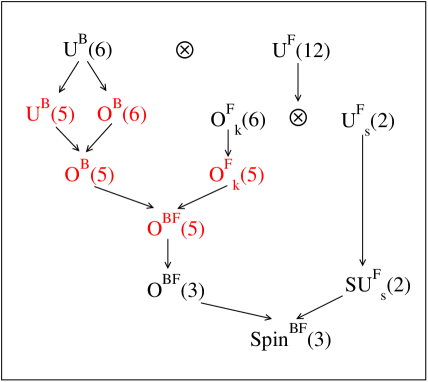
Figure 2: The lattice of algebras involved in the IBFM Hamiltonian (18).

The corresponding spectrum is given in the lower frame of Fig. 1. A number N=7 of bosons is assumed as a typical value. Other choices of N do not alter the qualitative behaviour of our results. With the choice N=7 the critical point occurs at $x_{crit}=\frac{4N-8}{5N-8}=\frac{20}{27}\approx 0.74$. In the Hamiltonian the values for $k$ and $k^{\prime}$ have been assumed to be equal to the corresponding values in the E(5/12) case presented in the upper frame.

The spectrum has a structure that clearly resembles the one obtained within the E(5/12) model (upper frame). Energies of selected states in the two models are compared in Table 1. As noted before, in the E(5/12) model all states with $\tau_{1}^{F}$=0 (i.e. with the odd particle in the j=1/2 state) have precisely the same energies as the states in the even E(5) model. Similarly, in the IBFM these states have the same energy of the corresponding states in the boson Hamiltonian (15). The agreement for the energies of these states in E(5/12) and IBFM is therefore that already discused in ref.beta4 for the bosonic part. Excited bands with $\tau_{1}^{F}$=1 (i.e. with the odd particle in the j=3/2,5/2 states), on the other hand, seem to be somewhat compressed in E(5/12) with respect to the IBFM.

The same kind of agreement is also present in the electromagnetic transitions. Consistently with the choice presented in the E(5/12), we assume in the IBFM as E2 transition operator just the boson (collective) quadrupole operator, i.e. $\hat{T}^{E2}~{}=~{}\hat{Q}_{B}$. The order of magnitude of the different B(E2) values are reflected in different thickness and styles of the arrows shown in Fig. 1. Given the choice of the IBFM Hamiltonian (18) the same selection rules valid in the E(5/12) model also apply to the ($\tau_{1}^{B},\tau_{1}^{F},\tau_{1},\tau_{2})$ quantum numbers of initial and final states in the IBFM approach. The B(E2) values of selected transitions are explicitly given in the figure. All B(E2) values are normalized to 100 for the first 5/2 - 1/2 transition. Similarly to what happens for the energies of the levels, the overall behaviour is very similar to that of the E(5/12).

Level	Energy	Energy
$~{}~{}\xi,\tau_{1}^{B},\tau_{1}^{F}(\tau_{1},\tau_{2})~{}~{}$	E(5/12)	IBFM
1,1,0 (1,0)	1.00	1.00
1,2,0 (2,0)	2.20	2.30
2,0,0 (0,0)	3.03	2.86
1,0,1 (1,0)	2.20	2.69
1,1,1 (1,1)	3.00	3.82

Table 1: Energies of selected states in E(5/12) and IBFM (normalized to the first excited multiplet). The values $k=-1/4,k^{\prime}=5/2$ have been used in both Hamiltonians (LABEL:Hbohr) and (18). In the IBFM calculation, a number N=7 of bosons has been used.

In this letter we have presented an analytic model (E(5/12)) for the critical point of the phase transition from spherical to $\gamma$-unstable shapes in odd nuclei, i.e. a mixture of fermion and boson degrees of freedom. In the model the fermion is allowed to occupy many single particle orbitals. Spectrum and intensities of electromagnetic transitions have been compared with those obtained within the Interacting Boson Fermion Model showing comparable behaviours. We think that our model, which includes the more realistic many j-orbits case compared with the E(5/4) model, should offer more chances for the occurrence of critical point symmetries in odd nuclei, in addition to those already found in the case of even nuclei.

This work has been partially supported by the Spanish Ministerio de Educación y Ciencia and by the European regional development fund (FEDER) under project number FIS2005-01105, and by INFN. Andrea Vitturi acknowledges financial support from SEUI (Spanish Ministerio de Educación y Ciencia) for a sabbatical year at University of Sevilla.

References

- (1) F. Iachello, Phys. Rev. Lett. 95, 052503 (2005)
- (2) F. Iachello, in Symmetries and low-energy phase transitions in nuclear structure physics, Camerino, 2005, Universitá degli Studi di Camerino, ed. G. Lo Bianco
- (3) M.A. Caprio and F. Iachello, Nucl. Phys. A (2006), doi:10.1016/j.nuclphysa.2006.10.032
- (4) M.S. Fetea et al., Phys. Rev. C 73, 051301(R) (2006)
- (5) F. Iachello and P. Van Isacker, The Interacting Boson Fermion Model, Cambridge University Press, (1991)
- (6) P. Van Isacker, A. Frank and H-Z. Sun, Ann. Phys. (N.Y) 157, 183 (1984)
- (7) J. M. Arias, C. E. Alonso, A. Vitturi, J. E. García-Ramos, J. Dukelsky, and A. Frank, Phys. Rev. C 68, 041302(R) (2003)
- (8) C.E. Alonso, J.M. Arias, L. Fortunato and A. Vitturi, Phys. Rev. C 72, 061302(R) (2005)
- (9) C. E. Alonso, J. M. Arias, and A. Vitturi, Phys. Rev. C 74, 027301 (2006)
- (10) J. Jolie, P. Cejnar, R.F. Casten, S. Heinze, A. Linnemann, and V. Werner, Phys. Rev. Lett. 89, 182502 (2002)
- (11) F. Iachello, Phys. Rev. Lett. 85, 3580 (2000)
- (12) P.S. Turner and D.J. Rowe, Nucl. Phys. A756, 333 (2005)
- (13) C.E. Alonso, in Proceedings of 3rd Workshop on shape phase transitions and critical point phenomena in nuclei, Athens, 2006, ed. D. Bonatsos, http://www.inp.democritos.gr/lenis/
- (14) J. Jolie, S. Heinze,, P. Van Isacker, and R.F. Casten, Phys. Rev. C 70, 111305(R) (2004)